Early supernovae light-curves following the shock-breakout

Abstract

The first light from a supernova (SN) emerges once the SN shock breaks out of the stellar surface. The first light, typically a UV or X-ray flash, is followed by a broken power-law decay of the luminosity generated by radiation that leaks out of the expanding gas sphere. Motivated by recent detection of emission from very early stages of several SNe, we revisit the theory of shock breakout and the following emission, paying special attention to the photon-gas coupling and deviations from thermal equilibrium. We derive simple analytic light curves of SNe from various progenitors at early times. We find that for more compact progenitors, white dwarfs, Wolf-Rayet stars (WRs) and possibly more energetic blue-supergiant explosions, the observed radiation is out of thermal equilibrium at the breakout, during the planar phase (i.e., before the expanding gas doubles its radius), and during the early spherical phase. Therefore, during these phases we predict significantly higher temperatures than previous analysis that assumed equilibrium. When thermal equilibrium prevails, we find the location of the thermalization depth and its temporal evolution. Our results are useful for interpretation of early SN light curves. Some examples are: (i) Red supergiant SNe have an early bright peak in optical and UV flux, less than an hour after breakout. It is followed by a minimum at the end of the planar phase (about 10 hr), before it peaks again once the temperature drops to the observed frequency range. In contrast WRs show only the latter peak in optical and UV. (ii) Bright X-ray flares are expected from all core-collapse SNe types. (iii) The light curve and spectrum of the initial breakout pulse holds information on the explosion geometry and progenitor wind opacity. Its spectrum in more compact progenitors shows a (non-thermal) power-law and its light curve may reveal both the breakout diffusion time and the progenitor radius.

1 Introduction

A breakout of a shock through the stellar surface is predicted to be the first electro-magnetic signal heralding the birth of a supernova (SN) (Colgate, 1974; Falk, 1978; Klein & Chevalier, 1978; Imshennik, Nadezhin & Utrobin, 1981; Ensman & Burrows, 1992; Matzner & McKee, 1999). Before breakout the shock is propagating through the opaque stellar envelope. The shock is radiation dominated (i.e., the energy density behind the shock is dominated by radiation) and it accelerates while propagating through the decreasing density profile of the envelope, leaving behind the shock an expanding radiation dominated gas. Following the shock breakout, photons continue to diffuse out of the expanding stellar envelope producing a long lasting emission that slowly decays with time (e.g., Grassberg, Imshennik & Nadyozhin, 1971; Chevalier, 1976, 1992; Chevalier & Fransson, 2008; Piro, Chang & Weinberg, 2009). The typical frequency of the breakout emission ranges from far ultra-violet to soft $\gamma$-rays in core collapse SNe, and as we show here, is in $\gamma$-rays in type Ia SNe. The typical frequency of the following emission decreases to the visible-near UV bands after a day. The energy released during the breakout increases with the progenitor radius and can reach $\sim 0.1\%$ of the SN explosion energy in a red supergiant. The luminosity of core collapse SNe after a day is $\sim 10^{41}-10^{42}{\rm~{}erg/s}$. Thus, the shock breakout and the emission through the first day can be detected out to the nearby Universe, but without any preceding knowledge of where to look, their detection is challenging. Nevertheless, the search worth the effort as this emission bears direct information on the properties of the progenitor and the explosion, which are difficult to obtain in any other way.

The development during the recent decade of sensitive UV, X-ray and soft gamma-ray detectors, with relatively large fields of view, lead to the discovery of several shock breakout candidates (Campana et al., 2006; Soderberg et al., 2008; Gezari et al., 2008; Schawinski et al., 2008; Modjaz et al., 2009). Motivated by these, and by the rising potential for future detection of shock breakouts from various progenitors, we revisit this topic. We develop an analytic model that provides light curves (luminosity and temperature) starting from the breakout, through the quasi-planar expansion phase to the spherical expansion phase, until recombination and/or radioactive decay start playing a significant role. These phases were explored in previous works, where the most updated analytic study of the spherical phase was carried-out by Chevalier (1992); Chevalier & Fransson (2008), and Waxman, Mészáros & Campana (2007); Rabinak & Waxman (2010). The study of the planar phase was carried out only very recently by Piro, Chang & Weinberg (2009) in the context of Type Ia shock breakout. The advantage of our model is that we follow the photon-gas coupling within the expanding gas. At each stage of the evolution we find the location at which the observed temperature is determined. We find whether the radiation at this place is in thermal equilibrium or not and calculate the observed temperature. It turns out that the temperature evolution during the planar phase and the early spherical phase depends strongly on the thermal equilibrium of the radiation just behind the shock in the breakout layer. In radiation dominated shocks, radiation is out of thermal equilibrium if the shock velocity is high enough (Weaver, 1976), which is the case in shock breakout from more compact progenitors and more energetic explosions (Katz, Budnik & Waxman, 2010). We provide the first calculation (analytic or numerical) of the light curve in case that the observed radiation is out of thermal equilibrium at the source. We also carry out the first analytic calculation of the evolution of the location of the thermalization depth, through the different phases, when the radiation is in thermal equilibrium. We use our model to examine the light curve and spectrum of the initial pulse that is strongly affected by light travel time effects and opacity of the progenitor stellar wind. Finally, we use our model to explore the properties of early SNe light curves resulting from various progenitor types including red supergiants (RSG), blue supergiants (BSG), Wolf-Rayet stars (WR) and white dwarfs (WD). We provide simple formula of early SN light curves for these different progenitors.

We present our model and its general results in section 2. The bolometric luminosity and spectrum of the initial pulse are discussed in section 3. Early SNe light curves resulting from various progenitors are presented in section 4. A reader that is interested only at the final light curves should go directly to this section. In section 5 we compare our calculations to previous analytic and numerical studies. We summarize our main results in section 6. We ignore in this paper any cosmological redshift effects.

2 Luminosity and observed spectrum following shock breakout

SN explosion drives a radiation dominated shock (i.e., the internal energy in the shock downstream is dominated by radiation) that propagates and accelerates through the decreasing density profile of the stellar envelope. The pre-explosion density profile near the stelar radius, $R_{*}$, can be approximated by a power-law $\rho\propto(R_{*}-r)^{n}$ where $r$ is the distance from the star center and $n\approx 1.5-3$, depending on the stellar properties. In such medium the blast-wave assumes a self similar profile in which the shock velocity $v\propto\rho^{-\mu}$, where $\mu$ is a very weak function of $n$ and for the relevant range of $n$ can be well approximated as a constant $\mu\approx 0.19$ (Sakurai, 1960). This purely hydrodynamic solution, which neglects heat conduction, holds as long as the distance to the stellar edge, $R_{*}-r$, is larger than the width of the radiation dominated shock, or equivalently as long as the optical depth for photons to escape the stellar envelope, $\tau(r)$, is larger than $c/v(r)$, where $c$ is the light speed. Once $\tau\approx c/v$ the shock ”breaks-out”, leaving behind an expanding hot gas-radiation sphere. We denote the conditions at the front shell of gas at the breakout time (where $\tau\approx c/v$ at the breakout) by subscript ₀, and call this shell the breakout shell. Given above assumptions our problem is completely defined by the following parameters of the breakout shell at the breakout time. The parameters of the inner gas layers are directly related to it.

• $v_{0}$: the velocity of the shock when it breaks out.

• $m_{0}$: the mass of the breakout shell.

• $d_{0}$: the initial width of the breakout shell.

• $R_{*}$: the radius of the star.

• $n$: the power law index describing the pre-explosion density profile, typically $1.5\leq n\leq 3$

Other characteristics of the breakout shell can be calculated from the above. For example,

• $\tau_{0}=\kappa_{T}m_{0}/R_{*}^{2}$ is the initial optical depth for Thompson scattering, where $\kappa_{T}$ is the Thompson cross section per unit of mass.

• $t_{0}=d_{0}/v_{0}$ is the initial dynamical time of the breakout shell. It is also its initial diffusion time.

• $E_{0}=m_{0}v_{0}^{2}$ is the initial thermal energy of the breakout shell.

Conceptually, it is useful to treat the whole expanding envelope as a series of successive shells. Any shell deeper than the breakout shell, can be characterized by its mass $m>m_{0}$. Sakurai (1960)’s hydrodynamic solution discussed above indicates that for these deeper shells

• $v=v_{0}(m/m_{0})^{-0.19n\over n+1}$ is the velocity of the shell of mass $m$.

• $d_{i}=d_{0}(m/m_{0})^{1\over n+1}$ is the width of a shell of mass $m$ at shock breakout.

• $E_{i}=mv^{2}=E_{0}(m/m_{0})^{1+0.62n\over n+1}$ is the internal energy of a shell of mass $m$ at shock breakout.

The subscript _i, for time dependent quantities, indicates initial values.

Initially, after shock crossing but before significant expansion, the thermal and kinetic energies in each shell are equal, hence the expression for the initial internal energy given above. Following shock breakout the stellar envelope expands and the width of each shell increases as it accelerates on the expense of the gas thermal energy. The acceleration ends once the shell width is multiplied several times, approaching a coasting velocity which is about twice its initial one (Matzner & McKee, 1999). Hence, up to a factor of order unity, the initial velocity right after the shock equals its final coasting velocity, $v$. The internal energy on the other hand falls as the volume of the shell increases.

Following shock breakout, photons continue to diffuse out of the expanding stellar envelope. Below we derive the luminosity and typical frequency of the diffusing photons. We focus on the early phases, where the gas ionization fraction is high and the opacity is dominated by Thomson scattering (e.g. over free-free absorption). This assumption breaks as soon as the observed temperature falls below about $1$ eV (the gas density at this point is $10^{-10}-10^{-9}{\rm~{}g/cm^{3}}$). We also neglect the drop in the number of free electrons due to recombination of fully ionized He (which takes place at a few eV), and assume that the energy injection due to recombination and radioactive decay are negligible. These conditions prevail from the shock breakout up until about a day after the explosion.

First, we derive the observed bolometric luminosity as a function of time. It is dictated by the hydrodynamics and Thompson scattering and does not depend on the thermal coupling between the diffusing radiation and the gas (at the stages of interest the shells are coasting and the hydrodynamics is decoupled from the radiation). Then, we discuss the radiation-gas coupling and derive the observed spectrum, both when the diffusing radiation is in thermal equilibrium and when it is not. We do not provide the radius of the photosphere (i.e., $\tau=1$) since it has no observable signature in the specific system at hand. Instead we provide the radius and mass of the location at which the luminosity is determined (see definition below), $\widehat{r}$ and $\widehat{m}$ and the radius and mass of the location at which the observed temperature (color) is determined, $r_{cl}$ and $m_{cl}$.

2.1 Luminosity

At any given time the observed luminosity is dominated by the innermost shell out of which photons can effectively diffuse, i.e. where the diffusion time is comparable to the time past since breakout, which is also the dynamical time. The reason is that the diffusion time from inner shells is longer and therefore their photons are confined and cannot be seen, while the radiation from outer shells already escaped the expanding gas and were observed at earlier times. The criterion that the diffusion time is comparable to the dynamical time is $\tau\approx c/v$. Thus, the bolometric luminosity at time $t$ is determined by the radiation energy in the shell that satisfies $\tau(t)\approx c/v$. We call this shell the luminosity shell, and denote $\widehat{x}$ as the parameter $x$ of this shell. The luminosity is given then by $\widehat{E}/t$.

To follow the evolution, we measure the time $t$ from breakout. The relevant parameters of a shell are the width $d$, velocity $v$, internal energy $E$, optical depth $\tau$, and photon diffusion time $t_{d}$, all of which, except for $v$, are time dependent ($v$ only increases by a modest factor from its initial value, and is approximated here as constant). The following relations holds for each shell at all times $t>t_{0}$:

$$\tau = \kappa_{T}\frac{m}{r^{2}}$$ (1)

$$t_{d} = \frac{\tau d}{c}$$ (2)

$$E = E_{i}\left(\frac{r^{2}d}{R_{*}^{2}d_{i}}\right)^{1/3}$$ (3)

$$d = d_{i}+vt\approx vt$$ (4)

$$r \approx R_{*}+vt$$ (5)

Our equation for the internal energy above assumes adiabatic expansion of a radiation dominated gas. It is therefore not valid for outer shells where $t>t_{d}$ which cooled radiatively. It is applicable from the luminosity shell and inward.

The hydrodynamic evolution has two phases - a planar phase and a spherical phase. The evolution of a shell is approximately planar as long as its radius did not double and it is spherical at later times. As we show below the breakout shell is also the luminosity shell while the evolution of the breakout shell is planar. Thus we separate the temporal evolution into two asymptotic regimes, $(t_{0}<)t\ll t_{s}$ and $t\gg t_{s}$, where $t_{s}=R_{*}/v_{0}$ is the time of transition between the planar and spherical geometries of the breakout shell.

During the planar phase $r\approx R_{*}$, implying a constant $\tau$. Since $d\propto t$ we obtain that $t_{d}/t$ is constant in time for all the shells during their planar evolution. As we have seen above at the beginning of the planar phase (i.e., $t=t_{0}$), the diffusion time equals the dynamical time only for the breakout shell. Therefore, the breakout shell is also the luminosity shell (i.e., $\widehat{m}\approx m_{0}$) throughout the planar phase. The implication is that throughout the planar phase we continue to observe photons from roughly the breakout shell. Adiabatic cooling then dictates

$$\widehat{E}(t<t_{s})\approx E_{0}(t/t_{0})^{-1/3}.$$ (6)

During the spherical phase $r\approx vt$ and the opacity is, $\tau\approx\tau_{0}\frac{m}{m_{0}}\left(\frac{R_{*}}{vt}\right)^{2}=\tau_{0}\left(\frac{m}{m_{0}}\right)^{\frac{1.38n+1}{n+1}}\left(\frac{t}{t_{s}}\right)^{-2}.$ The luminosity shell satisfies, by definition, $\widehat{t_{d}}=t$, which is equivalent to $\tau=c/v$. Combining these two equations for $\tau$, we find that at $t>t_{s}$ the luminosity shell evolves with $\widehat{m}\propto t^{\frac{2(n+1)}{1.19n+1}}$, $\widehat{v}\propto t^{-\frac{0.38n}{1.19n+1}}$, $\widehat{r}\propto t^{\frac{0.81n+1}{1.19n+1}}$, $\widehat{d}_{i}\propto t^{\frac{2}{1.19n+1}}$ and $\widehat{\tau}\propto t^{\frac{0.38n}{1.19n+1}}$. Using these relations, and following the adiabatic cooling of the shells we obtain

$$\widehat{E}(t>t_{s})\approx E_{0}\left(\frac{t_{s}}{t_{0}}\right)^{-1/3}\left(\frac{t}{t_{s}}\right)^{\frac{1.29n+5}{3(1.19n+1)}}.$$ (7)

The observed bolometric luminosity, given by $\widehat{E}/t$, is therefore:

$$L_{obs}\approx\frac{E_{0}}{t_{0}}\left\{\begin{array}[]{lr}\left(\frac{t}{t_{0}}\right)^{-4/3}&~{}~{}t<t_{s}\\ \left(\frac{t_{s}}{t_{0}}\right)^{-4/3}\left(\frac{t}{t_{s}}\right)^{-\frac{2.28n-2}{3(1.19n+1)}}&~{}~{}t>t_{s}\end{array}\right.$$ (8)

The ratio $E_{0}/t_{0}$ is simply the initial luminosity $L_{0}$. This bolometric luminosity falls as $t^{-4/3}$ in the planar phase and falls much more modestly as $t^{-0.17}$ to $t^{-0.35}$ (for $1.5\leq n\leq 3$) during the spherical phase. The total energy released in a logarithmic time unit, $Lt$, increases once the spherical phase sets on. The reason is that most of the energy in the shock is left behind it, in deeper more massive shells, as the shock accelerates (indeed we have seen that $E_{i}$ is an increasing function of $m$). Therefore inner shells, which were previously opaque, become transparent during the spherical phase and those contain increasing amount of energy.

The radius and mass of the luminosity shell are:

$$\widehat{r}\approx R_{*}\left\{\begin{array}[]{lr}1&~{}~{}t<t_{s}\\ \left(\frac{t}{t_{s}}\right)^{\frac{0.81n+1}{1.19n+1}}&~{}~{}t>t_{s}\end{array}\right.,$$ (9)

$$\widehat{m}\approx m_{0}\left\{\begin{array}[]{lr}1&~{}~{}t<t_{s}\\ \left(\frac{t}{t_{s}}\right)^{\frac{2(n+1)}{1.19n+1}}&~{}~{}t>t_{s}\end{array}\right..$$ (10)

2.2 Spectrum

Throughout the early phases that we consider here, the radiation dominates the heat capacity. Therefore, the luminosity derived above is independent of the thermal coupling between the photons and the gas (even a full coupling which equates the gas and radiation temperatures everywhere has a negligible effect on the total radiation energy). However, the optical depth of the luminosity shell is always much greater than unity ($\widehat{\tau}_{i}=\tau_{0}\gg 1$ and $\widehat{\tau}$ only increases, or remains constant, with time). Thus, the escaping photons would have many interactions with electrons as they cross the envelope until finally escaping from the layer where $\tau=1$. Therefore, while the total radiation energy is independent of the photons-electrons interaction, the typical energy of each of the escaping photons is dictated by their coupling to matter along their way from the luminosity shell outward.

At any given time the photon luminosity at $r>\widehat{r}$ is constant (given by equation 8). Therefore, there are two extreme possibilities. (1) No radiation process can significantly change the number of photons. Then, since photons dominate the heat capacity, both luminosity and photon number flux are fixed (independent of $r$ for $r>\widehat{r}$). Thus, the typical photon energy must be fixed. The typical temperature is thus given by the photons temperature $\widehat{T}$ of the luminosity shell. That temperature, in turn, would be dictated by the limited ability of radiation processes in the luminosity shell to create photons. (2) Some radiation process can create new photons, which can share the energy of the diffusing photons. Then the typical energy of the photons decreases as they diffuse out. The typical temperature then falls below the photons temperature of the luminosity shell. If such processes exist at some radius $r>\widehat{r}$, how low can the temperature drop? Photons would only be created up until the radiation thermalizes. Given that the luminosity is constant, and that the diffusion time is $\tau d/c$, the photon energy density for all shells external to the luminosity shell up until optical depth of unity is

$$\epsilon~{}(1\leq\tau\leq\widehat{\tau})\approx\frac{\widehat{L}\tau}{cr^{2}}.$$ (11)

The thermal equilibrium temperature given such energy density is

$$T_{BB}\equiv(\epsilon/a)^{1/4},$$ (12)

where $a$ is the radiation constant. The temperature will never drop below $T_{BB}$ since then photons would be absorbed rather than emitted. As we show below, shells that can generate enough photons to affect the photons temperature on their diffusion out of the luminosity shell, will gain full thermal equilibrium, while shells that are out of thermal equilibrium do not affect the radiation temperature at all.

To clarify, we provide an alternative description of the two options discussed above. As long as the radiation and the gas are in thermal equilibrium (i.e, $\epsilon\propto T^{4}$), the photon number flux increases with $r$. Thus, the gas at $r>\widehat{r}$ must generate photons at a sufficient rate, and share the energy of the outgoing photons with the generated photons, in order to keep the radiation in thermal equilibrium temperature, $T_{BB}$. The observed temperature, is determined then by the outermost shell (at $r\geq\widehat{r}$) that is in thermal equilibrium. If, on the other hand, none of the shells at $r\geq\widehat{r}$ is in thermal equilibrium then $T_{obs}=\widehat{T}\gg\widehat{T}_{BB}$. Note that we refer here to the typical photon energy as the radiation temperature also when the radiation is out of thermal equilibrium.

We note that the relation $L=4\pi\sigma r^{2}T^{4}$, which is sometime used in the context of shock breakout, is wrong at any radius if $kT$ is the typical photon energy at radius $r$ ($\sigma$ is the Stefan-Boltzmann constant). The reason is that this equation, which relates luminosity, radius and temperature at the point where $\tau\approx 1$, assumes that the radiation is in thermal equilibrium at this point, while at the regime we discuss here it is never the case. At early times the optical depth is dominated by Thomson scattering, which conserves photon number. Therefore, as a typical photon should be absorbed at least once in shells that can keep thermal equilibrium, the shell at $\tau=1$ is always out of thermal equilibrium and it plays no roll in determining neither the temperature nor the luminosity.

Below we follow the photon-electron coupling in the different regimes and determine the time dependent observed temperature as function of initial conditions. We show that the observed temperature can assume radically different evolution between cases where the breakout shell is initially in equilibrium and cases where it is not. We stress that we use the term observed temperature to denote the typical energy of the observed photons also when the radiation is out of thermal equilibrium and the spectrum is not a blackbody. The observed temperature is often called color temperature when radiation is in thermal equilibrium (to separate it from the effective temperature, which we ignore throughout the paper since it is not an observable). We denote the shell at which the observed temperature is determined as the color shell. The color shell is the thermalization depth when thermal equilibrium is achieved, and as we show below the color shell is the luminosity shell when it is not.

2.2.1 photon-electron coupling and thermal equilibrium

The main processes that typically couple the gas and the radiation, at the physical conditions of interest, are free-free and bound-free emission and absorbtion and Compton or inverse Compton scattering. The importance of the free-free coupling, compared to bound-free coupling, depends on the metalicity, where in low metalicity environments the free-free process is more dominant while in high metalicity it is the bound-free. We assume here that free-free process dominate and discuss briefly the effects of bound-free coupling later.

Consider an isolated shell with a radiation dominated energy density $\epsilon$, which generates its own photons by free-free emission. Now assume that initially, even though it is radiation dominated, it does not have enough photons to be in thermal equilibrium. The radiation temperature is $T>T_{BB}$ and the hot photons must “cool”, by sharing their energy with newly generated photons, for the system to approach thermal equilibrium. This is achieved by emission from electrons. The energy content of these electrons is negligible, but we assume that they can constantly gain energy from the photons an remain at the radiation temperature (this assumption is justified in appendix B). In this way, the energy of the existing photons is shared with that of the new photons that are constantly generated by free-free emission. Then, given a sufficiently long time, the number density of generated photons is $n_{BB}\approx aT_{BB}^{4}/3kT_{BB}$ and thermal equilibrium is achieved. Therefore, the time required to achieve thermal equilibrium in the shell is roughly $n_{BB}/\dot{n}_{ph,ff}(T_{BB})$, where $\dot{n}_{ph,ff}$ is the rate, per unit volume, at which free-free emission generates photons with energy $h\nu\approx 3kT$.

In each shell that generates its own photons the time available to obtain thermal equilibrium is the time photons are confined to the shell, i.e., $\min\{t,t_{d}\}$. We, therefore, define a thermal coupling coefficient in the expanding gas:

$$\eta \equiv \frac{n_{BB}}{\min\{t,t_{d}\}~{}\dot{n}_{ph,ff}(T_{BB})}$$ (13)

$$\approx \frac{7\cdot 10^{5}{\rm~{}s~{}}}{\min\{t,t_{d}\}}\left(\frac{\rho}{10^{-10}{\rm g/cm^{3}}}\right)^{-2}\left(\frac{kT_{BB}}{100eV}\right)^{7/2}.$$

where we approximate $\dot{n}_{ph,ff}\approx 3.5\cdot 10^{36}{\rm s^{-1}~{}cm^{-3}~{}}\rho^{2}T^{-1/2}$. $\rho$ is mass density (in ${\rm g~{}cm^{-3}}$) and $k$ is the Boltzmann constant. In the definition of $\eta$ we do not include Comptonization of low energy photons, which for the physical systems of interest becomes important only when the radiation is out of thermal equilibrium (see below). $\eta$ of the breakout shell at the initial time $t_{0}$ is then approximated by

$$\eta_{0}\approx 0.2\left(\frac{v_{0}}{10^{4}~{}{\rm km/s}}\right)^{15/4}\left(\frac{\rho_{0}}{10^{-9}~{}{\rm g/cm^{3}}}\right)^{-1/8}.$$ (14)

We took here into account the fact that the shock compresses the gas by a factor of $7$ and we used the relation $T_{BB,0}\approx(\rho_{0}v_{0}^{2}/a)^{1/4}$ (see also Katz, Budnik & Waxman 2010). The criterion for thermal equilibrium behind the shock at the breakout is $\eta_{0}<1$, which can be translated to a limit on the the breakout velocity (Weaver, 1976; Katz, Budnik & Waxman, 2010): $v_{0}<15,000{\rm~{}km/s}$ with a negligible dependence on $\rho_{0}$ (as $\rho_{0}^{1/30}$). In case that bound-free emission dominates over free-free emission $\eta_{0}$ can be smaller by up to an order of magnitude (see section 2.2.5).

For $\eta<1$, the radiation is in thermal equilibrium and the temperature is $T_{BB}$. Due to the relation between absorbtion and emission $\eta\approx 1$ is also the requirement that a photon with $h\nu=3kT_{BB}$ is absorbed on average once by free-free process during the available time. Thus, if $t_{d}\leq t$ then $\eta=1$ is equivalent to $\tau_{abs}\tau\approx 1$ where $\tau_{abs}$ is the free-free absorption optical depth for photons with $h\nu=3kT_{BB}$.

If $\eta>1$ then free-free processes are not enough to couple the electrons to the radiation in the shell. Moreover, not enough photons are generated at $h\nu\sim 3kT$ to obtain thermal equilibrium. However, if Compton scattering provides enough coupling so the electrons follow the radiation temperature, then the temperature $T$ is determined by the total number of photons that are generated at $h\nu\sim 3kT$ or that are generated at lower frequency, but can be Comptonized to an energy $3kT$. Then free-free emission generates photons until the temperature satisfies $\epsilon/3kT=\min\{t,t_{d}\}~{}\dot{n}_{ph,ff}(T)\xi(T)$, where $\dot{n}_{ph,ff}$ accounts only for generation of photons at $h\nu\approx 3kT$ while $\xi(T)$ account for photons that are generated at lower frequencies and Comptonized to temperature $T$. Therefore, $\dot{n}_{ph,ff}(T)\xi(T)$ is the total production rate of photons that can equally share the energy in the shell. Since free-free emission produces roughly a constant number of photons for every decade of energy below $kT$, the Comptonization correction factor $\xi$ is logarithmic. If no photons can be Comptonized then $\xi=1$, while if Comptonization is important $\xi$ may be much larger than unity. Writing this condition in terms of $\eta$ we find that if $\eta>1$ then $T\xi(T)^{2}=T_{BB}\eta^{2}$.

The availability of a low energy photon for computerization is discussed by Weaver (1976). At the temperature and density range of interest ($0.1-50$ keV and $\sim 10^{-8}-10^{-10}{\rm~{}gr/cm^{3}}$) it is determined by the requirement that the photon energy can be doubled before it is re-absorbed by free-free process. The ratio between $T$ and the lowest energy photon that can be Comptonized is then (Weaver, 1976):

$$y_{max}\equiv\frac{kT}{h\nu_{min}}=3\left(\frac{\rho}{10^{-9}~{}{\rm g/cm^{-3}}}\right)^{-1/2}\left(\frac{T}{\rm 100eV}\right)^{9/4}$$ (15)

Using the approximated rate, per unit volume per unit of $y\equiv h\nu/kT$, at which free-free emission generates photons (Svensson, 1984) we find that for $y_{max}>1$ the number of generated photons that can be Comptonized to $kT$ is larger by a factor $\int_{\frac{1}{y_{max}}}^{1}(0.8-\ln[y])\frac{dy}{y}$ than the number of photons that free-free emission generates at $\approx kT$. Thus for $y_{max}>1$:

$$\xi(T)\approx\max\left\{1,\frac{1}{2}\ln[y_{max}]\left(1.6+\ln[y_{max}]\right)\right\}.$$ (16)

If $y_{max}<1$ then inverse compton does not contribute to the number of photons, implying $\xi=1$. All together the logarithmic correction to the number of photons, $\xi$, ranges between $\xi=1$ at $T\lesssim 100$ eV to $\xi\approx 100$ at $T=50$ keV. Therefore, since in the systems of interest $T_{BB}\lesssim 100$ eV Comptonization becomes important, and cannot be neglected, only once the radiation is out of thermal equilibrium.

In summary, an isolated shell would arrive to a temperature of:

$$T=T_{BB}\begin{cases}\frac{\eta^{2}}{\xi(T)^{2}}&\eta>1\\ 1&\eta<1\end{cases}$$ (17)

If $\eta<1$ the spectrum is a blackbody. When $\eta>1$ the spectrum is an optically thin thermal free-free emission (with electrons at temperature $T$), which is modified by Comptonization. It is therefore a Wien spectrum (determined by the number of photons) at high frequencies and thermal spectrum (with $T$) at low frequencies.

Equation 17 assumes that electrons and photons have the same temperature through the whole evolution. This is clearly the case after thermal equilibrium is obtained and while $\eta<1$, since free-free emission and absorbtion keep the electrons and photons tightly coupled. In case that photons are out of thermal equilibrium they approach equilibrium by “cooling” via Compton scattering. This scattering is the heating source of the electrons, while the main electron cooling source is free-free emission. Therefore equation 17 assumes that the electron cooling is the slower process. In appendix B we show that this is generally true in the cases of interest, and that it may be marginally violated only in a small region of the relevant parameter phase space, in which case the modifications are likely to be small. Therefore we assume that electrons and photons have the same temperature in shells that generate their own photons and that equation 17 is always valid in these shells.

Equation 17 neglects relativistic effects (pair production, relativistic bremsstrahlung, etc.) and is, therefore, accurate only for $T\lesssim 50$ keV (Weaver, 1976; Svensson, 1984). We do not calculate here the exact temperature when eq. 17 predicts higher temperature. In this case pair production will result in a lower temperature than eq. 17 predicts. In SNe, where the velocities are at most mildly-relativistic, the temperature should fall within the range of soft gamma-ray detectors, $\sim 50-200$ keV, when pair production is important (Katz, Budnik & Waxman, 2010).

2.2.2 Succession of Shells & The observed photon energy

In §2.2.1 we considered the evolution of the photon temperature in an isolated shell whose energy density $\epsilon$ is known. We have assumed that the initial number of photons was small, so that the shell itself produced all its photons. We now discuss the interaction between shells as the photons diffuse out. A shell external to the luminosity shell receives photons from inner shells. It could, potentially, lower the typical photon energy by sharing the energy of the incoming photons with more photons that are produced in the shell.

The effect of a shell on the radiation temperature depends on its thermal coupling coefficient:

$$\eta=\eta_{0}\left(\frac{T_{BB}}{T_{BB,0}}\right)^{7/2}\left(\frac{\rho}{\rho_{0}}\right)^{-2}\left(\frac{\min\{t,t_{d}\}}{t_{0}}\right)^{-1}.$$ (18)

A shell cannot affect the observed temperature if it does not generate more photons than those arriving from inner layers. Since the energy flux, $L$, is independent of $r$ at $r>\widehat{r}$, the number flux that each shell can generate is inversely proportional to the typical photons energy it could generate, given by equation 17. For $\eta<1$ the number flux that a shell can generate is $L/(kT_{BB})$ while for $\eta>1$ it is $L/(kT_{BB}\eta^{2}\xi^{-2})$. $T_{BB}$ is a decreasing function of $r$, and therefore shells with $\eta<1$ increase the number flux while bringing the photons temperature to $T_{BB}$. On the other hand, as we show later, $T_{BB}\eta^{2}$ is an increasing function of $r$ (the variation of the logarithmic factor $\xi$ between shells can be neglected), and therefore, shells with $\eta>1$ cannot change the number flux of photons arriving from inner shells, and cannot modify the photon energies. Moreover, $\eta$ is an increasing function of $r$. Therefore, if the luminosity shell is out of thermal equilibrium, i.e., $\widehat{\eta}>1$, then all external shells have $\eta(m<\widehat{m})>1$. It follows, that the only shell which affects the temperature when $\widehat{\eta}>1$ is the luminosity shell, which is generating its own photons.

The observed temperature is therefore:

$$T_{obs}=\left\{\begin{array}[]{lr}\frac{\widehat{\eta}_{c}^{2}}{\widehat{\xi}_{c}^{2}}\;\widehat{T}_{BB}&\widehat{\eta}>1\\ T_{BB}(\eta=1)&\widehat{\eta}<1\end{array}\right.$$ (19)

Where $\widehat{\eta}_{c}$ and $\widehat{\xi}_{c}$ are calculated for the shell that is currently the luminosity shell, at the point where the photon number in the shell was determined. Note that in case that $\widehat{\eta}<1$ the color shell is exterior to the luminosity shell, where $t_{d}\leq t$. Therefore the criterion $\eta=1$ is equivalent to $\tau_{abs}\tau\approx 1$, which is a criterion for departure from thermal equilibrium used in stellar envelope calculations, and in some of the works on shock breakouts (e.g., Ensman & Burrows, 1992).

$T_{obs}$ is the typical photon energy of the observed radiation, but the observed spectrum is not necessarily a blackbody. The spectrum of the radiation at the color shell is determined only by itself and is therefore that of an isolated shell with temperature $T_{obs}$ (see the description below equation 17). As discussed above, outer shells do not affect the number of photons with energy $h\nu\gtrsim kT_{obs}$, however they may contribute to the number of photons with energy $h\nu<kT_{obs}$, thereby modifying the low energy spectrum. We do not calculate here this modification.

In the following sections we calculate the observed temperature by first finding $T_{BB}$ in each shell. For shells external to the luminosity shell it is found using equation 8 and the relation $\epsilon\approx L\tau/cr^{2}$. For inner shells it is determined by the adiabatic cooling during the expansion following the shock passage. Then we use equation 13 to calculate $\eta$ and equation 19 to find $T_{obs}$. We define the color radius to be the radius at which the observed temperature is determined (i.e., the radius of teh color shell), namely $r_{cl}=\max\{\widehat{r},r(\eta=1)\}$. We define $m_{cl}$ as the color shell mass. i.e., $m(r>r_{cl})$. Note that we do not discuss the radius of the photosphere where $\tau=1$, since it has no observable consequence or physical importance in the context of early SN light curves.

2.2.3 The temperature during the planar phase ($t_{0}<t<t_{s}$)

As discussed above (section 2.1), the optical depth of each shell is fixed during the planar evolution and the breakout shell is also the luminosity shell. Therefore, the observed temperature can only be determined by the breakout shell or by shells that are further out (i.e., $m\leq m_{0}$). Unfortunately, the hydrodynamic evolution of these shells is uncertain, as it depends on the poorly understood details of the radiation dominated shock front as it breaks out of the envelope. As a working assumption, we take the density profile at $m<m_{0}$ during the whole planar phase to be similar to the pre-shock profile, i.e., $\rho=\rho_{i}d_{0}/v_{0}t$. We verify later that other reasonable profiles do not strongly affect the conclusions. Having $\rho(m,t)$ we use equation 11 to find $T_{BB}(m,t)$ and then equation 18 (noting that here $t_{d}\leq t$) to obtain:

$$\eta(m\leq m_{0})=\eta_{0}\left(\frac{m}{m_{0}}\right)^{-\frac{17n+9}{8(n+1)}}\left(\frac{t}{t_{0}}\right)^{-1/6}$$ (20)

Thus, the thermal coupling increases slowly, but monotonically, with mass and time, everywhere. This is true for any profile where the density drops with radius. The number of photons in the luminosity shell increases continuously if it is out of thermal equilibrium (i.e., $\widehat{\eta}$ decreases with time so $\widehat{\eta}_{c}=\widehat{\eta}(t)$), and following equations 19 and 20 the observed temperature at $t_{0}<t<t_{s}$ is:

$$T_{obs}=\left\{\begin{array}[]{lc}T_{obs,0}\left(\frac{\widehat{\xi}(T_{obs})}{\xi_{0}(T_{obs,0})}\right)^{-2}\left(\frac{t}{t_{0}}\right)^{-2/3}&\widehat{\eta}>1~{}(t<t_{0}\eta_{0}^{6})\\ T_{BB,0}\eta_{0}^{~{}\frac{2(n+1)}{17n+9}}\left(\frac{t}{t_{0}}\right)^{-\frac{2}{3}\frac{9n+5}{17n+9}}&\widehat{\eta}<1~{}(t>t_{0}\eta_{0}^{6})\end{array}\right..$$ (21)

The value of $T_{obs,0}$ when $\eta_{0}>1$ is calculated by solving the implicit equation 17 for $T$ using $\eta_{0}$ and $\xi_{0}(T_{obs,0})$. Note that for $\widehat{\eta}>1$ equation 21 is implicit due to the dependence of $\widehat{\xi}$ on $T_{obs}$. We solve for $\widehat{\xi}$ by plugging $\rho=\rho_{0}(t_{0}/t)$ in equation 15. $\widehat{\xi}$ is continuously decreasing during the planar phase, but its decay is not described by a power-law and so is the decay of $T_{obs}$. Nevertheless the temperature instantaneous power-law decay index $\alpha=d\ln(T_{obs})/d\ln(t)$ is bounded between that of an adiabatic cooling and that of a constant $\xi$, i.e., $1/3<\alpha<2/3$. The drop in $\xi$ is smaller when $\eta$ is larger, implying that $\alpha$ decreases with $\eta$.

The radius of the color shell is roughly constant during the planar phase, $r_{cl}\approx R_{*}$. If $\eta_{0}<1$ then $m_{cl}$ depend strongly on the unknown density profile at $m<m_{0}$. If $\eta_{0}>1$ the photospheric mass is constant $m_{cl}=m_{0}$. We find that $T_{BB}\eta^{\;2}$ increases with the radius, in agreement with our assertion that shells external to the breakout shell that are out of thermal equilibrium, do not affect $T_{obs}$ since they generate less photons than those arriving from inner shells. Finally, we verify that taking other density profiles external to the breakout shell such as a steeper decreasing density ($\rho=\rho_{i}d_{i}/v_{0}t$) and a constant (in radius) density ($\rho=\rho_{0}d_{0}/v_{0}t$) do not significantly change equation 21 (the power-law indices when $\widehat{\eta}<1$ are changed by less than 0.1).

2.2.4 The temperature during the spherical phase $t>t_{s}$

The evolution of the spectrum during the early spherical phase depends strongly on whether the breakout shell is in thermal equilibrium at $t_{s}$. When it is, the color shell at $t_{s}$ is at $m<m_{0}$ and it quickly moves inward (in Lagrangian sense) to $m>m_{0}$. Following similar steps to those we used to derive equation 20 taking $\rho(m_{0}\leq m,t)$ we find

$$\eta(m_{0}\leq m)=\eta_{0}\left(\frac{t_{s}}{t_{0}}\right)^{-1/6}\left(\frac{t}{t_{s}}\right)^{\frac{42n+49}{12(1.19n+1)}}\left(\frac{m}{m_{0}}\right)^{-\frac{22.32n+17}{8(n+1)}}.$$ (22)

We consider here only $m<\widehat{m}$ where the time available for equilibrium is $t_{d}$. The color shell is at $m(\eta=1)$ and the observed temperature is:

$$T_{obs}(\widehat{\eta}<1) = T_{BB,0}\eta_{0}^{~{}\frac{2(1.76n+1)}{22.32n+17}}\left(\frac{t_{s}}{t_{0}}\right)^{-\frac{8.03n+6}{22.32n+17}}$$ (23)

$$\left(\frac{t}{t_{s}}\right)^{-\frac{18.48n^{2}+20.69n+6}{(1.19n+1)(22.32n+17)}}.$$

The color radius and the mass above it are

$$r_{cl}(\widehat{\eta}<1)\approx R_{*}\left(\frac{t}{t_{s}}\right)^{\frac{5.31n^{2}+9.09n+4.25}{(1.19n+1)(5.58n+4.25)}}$$ (24)

and

$$m_{cl}(\widehat{\eta}<1) = m_{0}~{}\eta_{0}^{\frac{2(n+1)}{5.58n+4.25}}\left(\frac{t_{s}}{t_{0}}\right)^{-\frac{n+1}{3(5.58n+4.25)}}$$ (25)

$$\left(\frac{t}{t_{s}}\right)^{\frac{7(6n+7)(n+1)}{6(1.19n+1)(5.58n+4.25)}}.$$

The optical depth at the color shell decreases with time roughly as $\tau_{cl}\propto m_{cl}^{2}/r_{cl}\propto t^{-0.4}$. Once $\tau_{cl}=1$ the opacity is not dominated anymore by Thomson scattering and our model assumptions break. Typically, however, the model assumptions break first by the temperature droping to $1$ eV (and recombination becoming important) while $\tau_{cl}>1$. Note that $r_{cl}(\widehat{\eta}<1)$ increases faster than $\widehat{r}$ with time. Thus, if the luminosity shell is at thermal equilibrium at a given time it will remain in equilibrium at any later time. Note also that equations 23-25 are valid whenever $\widehat{\eta}<1$, regardless of the value of $\widehat{\eta}$ at earlier times. A schematic light curve of this case is depicted in figure 1.

A very different evolution of $T_{obs}$ takes place if the luminosity shell is out of thermal equilibrium at $t_{s}$. Here evolution at the beginning of the spherical phase is determined by the fact that the thermal coupling of each shell increases (i.e., $\eta$ decreases) while its evolution is quasi-planar (i.e. $t<R_{*}/v$). On the other hand the thermal coupling becomes weaker during the spherical phase. Therefore, the photon production of shells that are out of equilibrium (i.e., $\eta>1$) is negligible during the spherical phase and the number of photons in such shells is determined by $\eta_{c}=\eta_{min}$, i.e. the minimal value of $\eta$ obtained when the shell just doubled its radius, and its thickness increased from the initial width $d_{i}$ to $R_{*}$ . There, using equation 18, with $(T_{BB}/T_{obs,0})^{4}\approx(d_{i}/R_{*})^{4/3}mv^{2}/m_{0}v_{0}^{2}$ and $\rho/\rho_{0}\approx mt_{0}/m_{0}t_{s}$, we obtain (noting that during the planar evolution for the relevant shells $t\leq t_{d}$),

$$\eta_{min}=\eta(t=R_{*}/v)=\eta_{0}\left(\frac{t_{0}}{t_{s}}\right)^{1/6}\left(\frac{m}{m_{0}}\right)^{-\frac{9.88n+5}{6(n+1)}}.$$ (26)

Thus, the observed temperature drops very quickly at the beginning of the spherical phase until $t_{1}\equiv t(\widehat{\eta}_{min}=1)$:

$$t_{1}=t_{s}\left[\eta_{0}\left(\frac{t_{0}}{t_{s}}\right)^{1/6}\right]^{\frac{3(1.19n+1)}{9.88n+5}}$$ (27)

Between $t_{s}$ and $t_{1}$ the value of $\widehat{\xi}_{c}$ is also dropping significantly until it becomes of order unity at $t_{1}$. Therefore $T_{obs}$ does not evolve as a power-law during this time, and we do not provide here a formula for its evolution. Nevertheless the drop in $T$ is very quick ($\propto t^{-5.3}$ when the evolution of $\widehat{\xi}_{c}$ is neglected) providing a strong observational signature, regardless of the exact decay rate.

At $t_{1}$ the observed radiation is in thermal equilibrium (i.e., $T_{obs}=\widehat{T}_{BB}$), although $\widehat{\eta}>1$, since the radiation was in thermal equilibrium at $t=R_{*}/\widehat{v}$ and equilibrium is kept through adiabatic cooling. The observed temperature during this phase, $\widehat{\eta}_{min}<1<\widehat{\eta}(t)$, is (note that $\widehat{\xi}_{c}=1$ at this time):

$$T_{obs}(t_{1}<t<t_{2})=T_{BB,0}~{}\eta_{0}^{2}\left(\frac{t_{s}}{t_{0}}\right)^{-2/3}\left(\frac{t_{1}}{t_{s}}\right)^{-\frac{21.27n+11}{3(1.19n+1)}}\left(\frac{t}{t_{1}}\right)^{-\frac{3n+2}{6(1.19n+1)}}$$ (28)

The relation $T_{obs}=\widehat{T}_{BB}$ holds until $t_{2}\equiv t(\widehat{\eta}=1)$. Since $\widehat{\eta}\propto t^{\frac{12.48n+1}{6(1.19n+1})}$ we find:

$$t_{2}=t_{s}\left[\eta_{0}\left(\frac{t_{0}}{t_{s}}\right)^{1/6}\right]^{\frac{6(1.19n+1)}{12.48n+1}}.$$ (29)

During the whole time that $\widehat{\eta}>1$ the color shell is also the luminosity shell ($r_{cl}=\widehat{r}$) and therefore:

$$r_{cl}(t_{s}<t<t_{2})=R_{*}\left(\frac{t}{t_{s}}\right)^{\frac{0.81n+1}{1.19n+1}}$$ (30)

and

$$m_{cl}(t_{s}<t<t_{2})=m_{0}~{}\left(\frac{t}{t_{s}}\right)^{\frac{2(n+1)}{1.19n+1}}.$$ (31)

At $t>t_{2}$ the color shell is exterior to the luminosity shell ($\widehat{r}<r_{cl}$) and is in thermal equilibrium. Thus $T_{obs}$, $r_{cl}$ and $m_{cl}$ at $t>t_{2}$ are given by equations 23-25. Finally, In all the different regimes of the spherical phase $T_{BB}\eta^{\;2}$ increases with the radius at $r>\widehat{r}$, implying that shells which are out of thermal equilibrium in this radii range do not affect $T_{obs}$. A schematic light curve in case that the luminosity shell is out of thermal equilibrium at $t_{s}$ is depicted in figure 1.

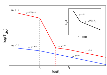
Figure 1: Main: A Schematic plot of the temperature evolution in the cases of $\eta_{0}>1$ (red line) and $\eta_{0}>1$ (blue line). The power-law indices indicated in the plot depend weakly on $n$ (see the text) and the values given here are very good approximations when $n$ ranges between $1.5$ and $3$. Inset: A Schematic plot of the bolometric luminosity evolution. The luminosity, unlike the observed temperature, is independent of the thermal coupling and the value of $\eta$.

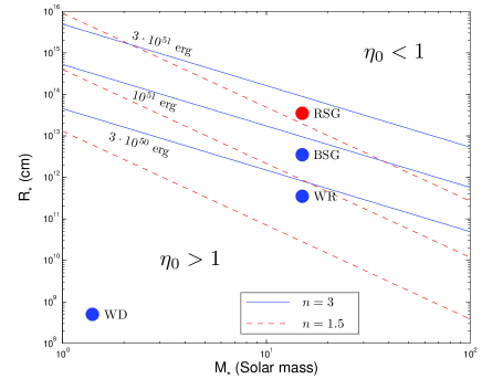
Figure 2: Main: Contours of $\eta_{0}=1$ in the $M_{*}$-$R_{*}$ plane for three different values of the explosion energy ($3\cdot 10^{50}$ erg, $10^{51}$ erg and $3\cdot 10^{51}$ erg), and two values of $n$ ($n=3$ [solid line] and $n=1.5$ [dashed line]). We used $\kappa=0.34{\rm~{}cm^{2}g^{-1}}$ and assume that free-free process dominates the emission and absorbtion. Above and to the right of each contour, i.e. the larger and more massive progenitors, $\eta_{0}<1$ and the radiation is at thermal equilibrium at the shock breakout time. Progenitors to the bottom and left of the contour (less massive and more compact) are out of thermal equilibrium during the breakout, and typically thermal equilibrium is gained only after the transition to the spherical phase. Typical $M_{*}$-$R_{*}$ of RSG, BSG, WR and WD progenitors are marked as well. RSGs (n=1.5) are in thermal equilibrium during breakout of typical SNe and are expected to fall out of equilibrium only if the SN kinetic energy is $\gtrsim 5\cdot 10^{51}$ erg. BSGs (n=3) are on the borderline and larger BSGs are expected to be in thermal equilibrium during breakout while less massive and compact BSGs don’t. WRs (n=3) and WDs are out of thermal equilibrium in typical SNe breakout.

2.2.5 The effect of bound-free absorbtion and emission

In our calculations above we assumed that free-free is the dominant emission and absorbtion process. This is the case in low metalicity progenitor envelopes ($\lesssim 0.1$ solar) but not in high metalicity ones ($\gtrsim$ solar). When bound-free dominates, the absorbtion coefficient, $\kappa_{bf}$, is a non-trivial function of the wavelength, temperature and density. Nevertheless, a rough estimate of the opacity at $\nu\approx kT/h$ show that the general dependence on $T$ and $\rho$ is similar to that of free-free, i.e, $\kappa_{bf}\propto\kappa_{ff}\propto\rho T^{-3.5}$ (e.g., Schwarzschild, 1958). Therefore, when bound-free dominates, thermalization is achieved faster (and kept for longer) by a factor $\kappa_{bf}/\kappa_{ff}$ implying that in each shell $\eta$ is reduced by this factor. Thus, all the equations derived above are valid after the definition of $\eta$ (eq. 13) and the value of $\eta_{0}$ (eq. 14) are divided by $\kappa_{bf}/\kappa_{ff}$ (ignoring the effect of the logarithmic factor $\xi$).

The correction to the observed temperature in case that the radiation is in thermal equilibrium ($\widehat{\eta}<1$) is small. The reason is that the dependence of $T_{obs}$ on $\eta_{0}$ is very weak (roughly as $\eta_{0}^{0.14}$), while in typical envelopes, which are dominated by Hydrogen or Helium, $\kappa_{bf}/\kappa_{ff}\lesssim 10$. This factor, however, is important in determining whether the radiation is in thermal equilibrium during the breakout and in calculating the temperature when it is not. Note that when the temperature is very high, $\gtrsim 10$ keV, the metals are fully ionized and bound-free process can be ignored regardless of metalicity.

3 The initial pulse

In previous sections we calculated the luminosity and temperature of the expanding gas as a function of time. The initial timescale is $t_{0}$, and both the luminosity and the typical photons energy evolve as power-laws of time for $t>t_{0}$. However, several effects can smear the observed flux at early times. Differences in the light travel time to the observer, asphericity of the explosion (e.g., Couch et al., 2010), or diffusion of the radiation through an optically thick surrounding such as thick wind blown by the progenitor before the explosion (e.g., Li, 2007). Below we discuss how light travel time and stellar wind shape the luminosity and spectrum of the initial pulse.

3.1 Luminosity

3.1.1 Light travel time of spherical explosion

Light travel time in a spherical explosion significantly affects the light curve and spectrum only at $t<R_{*}/c$ and it would be important only if $R_{*}/c>t_{0}$. The light crossing time is always shorter than $t_{s}$ ($R_{*}/c<R_{*}/v_{0}=t_{s}$), and therefore, its effects are important only during the planar phase. If light travel time shapes the initial pulse then for $R_{*}/c>t_{0}$, the observed flux rises over a timescale $t_{0}$ and remains roughly constant over a duration $R_{*}/c$. The observed luminosity during the initial pulse is $\sim L_{0}t_{0}c/R_{*}<L_{0}$. After this plateau, at $t>R_{*}/c$, the luminosity starts decreasing as $t^{-4/3}$ and is given again by equation (8) as light travel time matters no more. An example of such light curve can be seen in figure 5 where the WR X-ray luminosity is bolometric until $t_{s}=90$ s.

Note, that when light travel time shapes the initial pulse, then both $R_{*}$ and $t_{0}$ can be directly measured. The former is given by the duration of the initial pulse and the latter by its rise time. For more extended RSG progenitors, where $t_{0}$ may be comparable to, or exceed, $R_{*}$ (see appendix A) both the rise time and duration of the initial pulse are given by $t_{0}$ and the progenitor’s radius is not directly measurable.

The discussion above is focused on the bolometric luminosity. For observations at frequencies lower than the initial typical energy given by $T_{obs,0}$, the rise time will be longer than $t_{0}$ (assuming $t_{0}<R_{*}/c$). Depending on thermal equilibrium it is either $R_{*}/c$ or the time that the typical temperature falls into the the observed frequency window (see e.g., figures 3 and 4).

3.1.2 Winds

WR progenitors are surrounded by the thick stellar wind ejected during the WR phase. The optical depth of a wind is gained mostly close to its source, between $R_{*}$ and $2R_{*}$. Typical WR winds, are mildly optically thick, with optical depth that can be as high as $\tau_{w}\sim 1-10$ once the wind is fully ionized by the precursor of the breakout emission (Li, 2007). If the wind is very thick, $\tau_{w}\gg c/v_{sh}$ the radiation dominated shock would propagate in the wind as well and it should be treated in a similar way to our discussion in the previous sections. If $1\lesssim\tau_{w}\lesssim c/v_{sh}$ then photons diffuse through the wind without generating a radiative dominated shock. The energy output of the shock breakout is not affected but the arrival time of the photons to the observer is smeared over $\tau_{w}R_{*}/c$. The pulse rise and decay times are both $\tau_{w}R_{*}/c$. The information about $t_{0}$ is lost and so is the ability to measure $R_{*}$ directly.

3.2 Spectrum

3.2.1 Light travel time

If light travel time shapes the initial pulse, then at first, $t\sim t_{0}$, the spectrum is dominated by the emission from the shock front which is propagating in a decreasing optical depth during the breakout. The typical observed photon frequency is therefore $T_{obs,0}$. As time evolves, $t_{0}<t<R_{*}/c$, the spectrum broadens to include lower frequencies as well. During this time high frequency breakout photons, $T_{obs,0}$, continues to arrive from areas with longer travel time while lower frequency photons from the expanding gas are arriving from areas with shorter travel time. Ignoring light travel time effects we derived $T_{obs}=T_{obs,0}(t/t_{0})^{-\alpha}$, ($1/3<\alpha<2/3$), while $L=L_{0}(t/t_{0})^{-4/3}$ (see equations (21) and (8)). Thus, the spectrum of the initial pulse broadens in time to form a power-law,

$$F_{\nu}\propto\nu^{\frac{1}{3\alpha}-1},$$ (32)

over a frequency range that grows with time. Its upper frequency corresponds to the initial temperature $T_{obs,0}$ while the lower end of the power-law corresponds to the current (non delayed) temperature $T_{obs,0}(t/t_{0})^{-\alpha}$. The integrated spectrum of the initial pulse will show this power-law over a frequency range $kT_{obs,0}(ct_{0}/R_{*})^{\alpha}<h\nu<kT_{obs,0}$.

3.2.2 Wind

In the case of a mildly opaque wind ($1\lesssim\tau_{w}\lesssim c/v$) photons spend a time $\tau R_{*}/c$ diffusing through the wind, thereby erasing all the temporal details on shorter time scales. As a result the observed spectrum is given by $F_{\nu}\propto\nu^{\frac{1}{3\alpha}-1}$ over the frequency range $kT_{obs,0}(ct_{0}/\tau_{w}R_{*})^{\alpha}<h\nu<kT_{obs,0}$ right from the beginning.

Compton and inverse Compton scattering in the wind may also modify the photon’s energy. However, the number of collisions per photon is $\tau_{w}^{2}$, and the number of collisions needed to significantly change a photon energy is $m_{e}c^{2}/kT$. Since the winds we are dealing with have moderate optical depth and our temperature calculations are applicable to cases where $T\lesssim 50$ keV, scattering within the wind cannot make a significant change to the energy of such photons. Therefore this effect is not very important in the temperature range that we can calculate.

4 Early SNe light curves from various progenitors

Below we present early light curves (luminosity and spectrum) for different SN progenitors. We consider different progenitors of core-collapse SN: red supergiant (RSG), blue supergiant (BSG) and Wolf-Rayet (WR) stars. We also discuss the effect of deviation from thermal equilibrium on the signal that follows the shock breakout of type Ia SN presented in Piro, Chang & Weinberg (2009). The light curves are derived according to the results presented in previous sections, assuming that free-free is the dominant emission and absorbtion process, and the properties of the breakout shell given in appendix A.

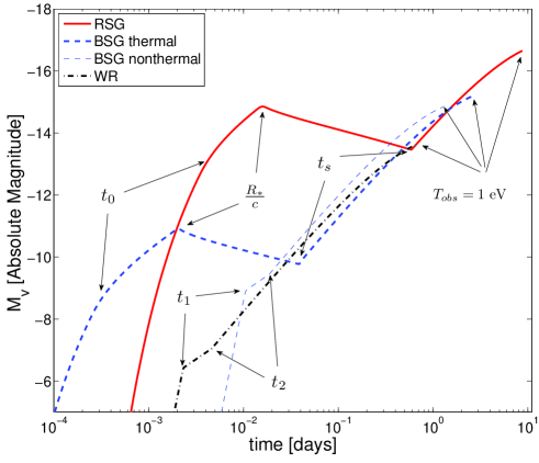
Figure 3: The optical light curve (in absolute V magnitude) following the shock breakout from RSG (solid line), BSG in thermal equilibrium (thick dashed line) and out of thermal equilibrium during the breakout (thin dashed line) and WR (dash-doted line). In all cases the explosion energy is $10^{51}$ erg. The progenitors radii are $500{\rm~{}R_{\odot}}$ (RSG), $70{\rm~{}R_{\odot}}$ (BSG thermal), $20{\rm~{}R_{\odot}}$ (BSG non-thermal) and $5{\rm~{}R_{\odot}}$ (WR). The progenitors masses are $15{\rm~{}M_{\odot}}$ in all cases except for the BSG thermal, where it is $25{\rm~{}M_{\odot}}$. The explosion is assumed to be spherical (light travel-time effects are included) and the pre-explosion stellar wind to be transparent. The source luminosity (before light travel time effects are included) at $t<t_{0}$ is approximated as $L_{0}\exp[1-\frac{t_{0}}{t}]$ (this is the luminosity of a radiation that leaks from the center of a static slab with a diffusion time $t_{0}$). The two thermal breakouts (RSG and BSG thermal) show a rising flux over a duration of $R_{*}/c$. The rise does not stop at $t_{0}$ since the optical band is below $T_{obs,0}$ (the optical is not the bolometric luminosity at early time). At $R_{*}/c$ the light curve start decaying until $t_{s}$, when the flux start rising again during the spherical phase up to the time when $T_{obs}$ drops to the observed frequency (not seen here because we cut the light curves at $T_{obs}=10^{4}$ K, see below). In the nonthermal breakouts the flux is strongly suppressed before $t_{s}$ since the temperature is very high (much higher than the optical). Then it rises very sharply up to $t_{1}$, when it falls into thermal equilibrium. At $t_{2}$ the flux joins the evolution of the thermal breakouts. Thus in the nonthermal breakouts the flux is rising continuously until the time that $T_{obs}$ drops to the observed frequency. We present light curves up to the point that $T_{obs}=10^{4}$ K, since this is roughly the point where recombination, which is neglected in our model, becomes important.

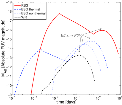
Figure 4: The FUV ($\nu_{{}_{FUV}}=2\cdot 10^{15}$ Hz) light curve in absolute AB magnitude, following the shock breakout from RSG (solid line), BSG in thermal equilibrium (thick dashed line) and out of thermal equilibrium during the breakout (thin dashed line) and WR (dash-doted line). The parameters and assumption are the same as in figure 3. The light curves evolution is similar to optical ones, with the difference that the second peak in the flux is observed earlier, once $T_{obs}$ get into the FUV range.

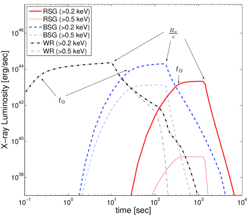
Figure 5: The total luminosity at frequencies $>0.2$ keV (thick lines) and $>0.5$ keV (this lines) following the shock breakout from RSG (solid lines), BSG in thermal equilibrium (dashed lines) and WR (dash-doted lines) stars. The parameters and assumption are the same as in figure 3. The depicted luminosity is the bolometric one, at $t<R_{*}/c$ in the WR and BSG cases, showing the light curve of the initial pulse in the case of a spherical explosion. The luminosity rises until $t_{0}$ when it becomes almost constant. The decay of the initial pulse starts at $R_{*}/c$.

4.1 Red supergiant

RSG is the progenitor of several members of the type II SN family. It has a convective envelope and its structure can be approximated using $n=1.5$. We assume a hydrogen envelope with cosmic abundances so the scattering cross-section per unit of mass is $\kappa=0.34{\rm~{}cm^{2}g^{-1}}$ (the dependence on $\kappa$ is weak). We consider a typical radius of $500R_{\odot}$ (a light crossing time of about $20{\rm~{}min}$) and a typical mass of $M_{*}=15M_{\odot}$. Following the initial pulse the luminosity evolves as:

$$L_{RSG}=\left\{\begin{array}[]{lr}\,\quad 10^{44}{\rm~{}erg/s~{}}M_{15}^{-0.37}R_{500}^{2.46}E_{51}^{0.3}t_{hr}^{-4/3}&t<t_{s}\\ 3\cdot 10^{42}{\rm~{}erg/s~{}}M_{15}^{-0.87}R_{500}E_{51}^{0.96}t_{d}^{-0.17}&t>t_{s}\end{array}\right.$$ (33)

where $R_{x}=R_{*}/xR_{\odot}$, $M_{x}=M_{*}/xM_{\odot}$, $E_{x}=E/10^{x}{\rm~{}erg}$ and $t_{hr}$ [$t_{d}$] is time in units of hours [days]. $E$ here is the explosion energy, not to be confused with the internal energy in the expanding shells. The transition between the planar and spherical phases takes place around

$$t_{s}=14{\rm~{}hr~{}}M_{15}^{0.43}R_{500}^{1.26}E_{51}^{-0.56}$$ (34)

The value of the thermal coupling parameter at the breakout is $\eta_{0}=0.06~{}M_{15}^{-1.72}R_{500}^{-0.76}E_{51}^{2.16}$. Therefore, the observed temperature is determined at the outermost shell which is in thermal equilibrium and it is given by eqs. 21 and 23:

$$T_{RSG}=\left\{\begin{array}[]{lr}10{\rm~{}eV~{}}M_{15}^{-0.22}R_{500}^{0.12}E_{51}^{0.23}t_{hr}^{-0.36}&t<t_{s}\\ \,\,\,3{\rm~{}eV~{}}M_{15}^{-0.13}R_{500}^{0.38}E_{51}^{0.11}t_{d}^{-0.56}&t_{s}<t\end{array}\right.$$ (35)

The ratio of the diffusion time of the breakout layer and the star light-crossing time is $ct_{0}/R_{*}=0.25M_{15}^{0.21}R_{500}^{1.16}E_{51}^{-0.79}$, implying that if the explosion is spherical the initial pulse has a rather well defined observed temperature of $T_{0,RSG}\approx 25{\rm~{}eV~{}}M_{15}^{-0.3}R_{500}^{-0.65}E_{51}^{0.5}$ and its rise time and duration are not too different.

Typical optical and FUV light curves are depicted in figures 3 and 4. The initial rise-time in both bands is $R_{*}/c$ (assuming a spherical explosion). Note that unlike the bolometric luminosity, here there is no plateau between $t_{0}$ and $R_{*}/c$ since the temperature is above the observed band at this time. Thus $t_{0}$ cannot be easily recovered from optical/UV light curves. The temperature remains above both the optical and the FUV bands during the planar phase and both light curves decay slowly. During the spherical phase the luminosity drops more slowly while $T_{obs}$ drops faster, as a result a break in the light curve is observed at $t\approx t_{s}$ and the optical flux starts rising. It peaks once $T_{obs}$ drops into the observed frequency range. The optical peak takes place after about two weeks. At that point the temperature is low enough so recombination, which we neglected, begins to be important. Therefore we terminate the light curve in the figures at earlier time when $T_{obs}=1$ eV.

The X-ray light curve is depicted in figure 5. $T_{RSG}(t_{0})$ is below the X-ray range and therefore only the initial pulse may be observed in soft X-rays. We assume here that the spectrum of the photons in the breakout layer is thermal, which implies that the initial X-ray pulse is very soft as the X-ray probes the exponential tail of the spectrum. Nevertheless, the energy in the soft X-ray flash from an RSG breakout is $\sim 3\cdot 10^{46}$ erg, which may be detectable to a substantial distance (possibly larger than that of a WR breakout X-ray flash).

Note that our analysis is appropriate only for RSGs with a density profile that drops sharply with $d$ near the edge, so the shock is accelerating before breakout. Our analysis also assumes that the width of the breakout shell is much smaller than the stellar radius ($d_{0}\ll R_{*}$). Stellar structure models such as those calculated by Gezari et al. (2008), using the KEPLER code (Weaver et al., 1978) and 3D hydrodynamics code (Freytag et al., 2002), are compatible with these assumptions. Our model assumptions, however, are incompatible with density profiles such as the one used by Schawinski et al. (2008), where the density of the envelope is very low ($\sim 10^{-11}{\rm gr/cm^{3}}$ at $0.5R_{*}$) and $d_{0}\sim R_{*}$.

4.2 Blue supergiant

BSG is also a progenitor of member(s) in the type II SN Family. It has a radiative envelope and is well approximated using $n=3$. We assume a hydrogen envelope with $\kappa$ similar to RSG. The typical radius is $50R_{\odot}$ giving $R_{*}/c\approx 2$ min. Following the initial pulse the luminosity evolves as:

$$L_{BSG}=\left\{\begin{array}[]{lr}2.5\cdot 10^{44}{\rm~{}erg/s~{}}M_{15}^{-0.33}R_{50}^{2.3}E_{51}^{0.34}t_{min}^{-4/3}&t<t_{s}\\ \,\,\,\,2\cdot 10^{42}{\rm~{}erg/s~{}}M_{15}^{-0.73}R_{50}E_{51}^{0.91}t_{hr}^{-0.35}&t>t_{s}\end{array}\right.$$ (36)

where $t_{min}$ is time in minutes. The transition between the planar and spherical phases takes place around

$$t_{s}=0.5{\rm~{}hr~{}}M_{15}^{0.41}R_{50}^{1.33}E_{51}^{-0.58}$$ (37)

The value of the thermal coupling parameter at the breakout is $\eta_{0}\approx 2~{}M_{15}^{-1.63}R_{50}^{-1.1}E_{51}^{2.24}$. Therefore, BSG progenitors are on the thermal coupling borderline. Thus, we expect both types of BSG shock breakouts, where less energetic explosions of more extended and massive BSGs will be in thermal equilibrium, while more energetic explosions of compact less massive BSGs will be out of thermal equilibrium. For example an $E=10^{51}$ erg explosion of a $R_{*}=70R_{\odot}$ and $M_{*}=25M_{\odot}$ progenitor has $\eta_{0}\approx 0.5$, and is therefore predicted to be in thermal equilibrium while if $R_{*}=20R_{\odot}$ and $M_{*}=10M_{\odot}$ then $\eta_{0}\approx 10$ and the breakout is predicted to be out of thermal equilibrium. Finally, in high metalicity envelopes bound-free emission dominates over free-free emission and $\eta_{0}$ is reduced (section 2.2.5). Therefore we provide here the temperature evolution for both thermal and non-thermal cases.

If the radiation is in thermal equilibrium at breakout time, $\eta_{0}<1$ (equations. 21 and 23) the observed temperature is:

$$T_{BSG}(\eta_{0}<1)=\left\{\begin{array}[]{lr}50{\rm~{}eV~{}}M_{25}^{-0.19}R_{70}^{0.06}E_{51}^{0.22}t_{min}^{-16/45}&t<t_{s}\\ 10{\rm~{}eV~{}}M_{25}^{-0.11}R_{70}^{0.38}E_{51}^{0.11}t_{hr}^{-0.61}&t_{s}<t\end{array}\right..$$ (38)

In case that the radiation is out of thermal equilibrium at breakout time, $\eta_{0}>1$, we use eqs. (21), (28) and (23) to find:

$$\begin{array}[]{l}T_{BSG}(\eta_{0}>1)\\ =\left\{\begin{array}[]{lr}150{\rm~{}eV~{}}M_{10}^{-1}R_{20}^{-0.1}E_{51}^{1.2}t_{min}^{-0.39}&t<t_{s}\\ 70{\rm~{}eV~{}}M_{15}^{-0.9}R_{20}^{-0.7}E_{51}^{1.1}\left(\frac{t}{t_{s}}\right)^{-2.1}&t_{s}<t<t_{1}\\ 15{\rm~{}eV~{}}M_{10}^{0.05}R_{20}^{0.25}E_{51}^{-0.1}\left(\frac{t}{15{\rm~{}min}}\right)^{-0.4}&t_{1}<t<t_{2}\\ 7{\rm~{}eV~{}}M_{10}^{-0.11}R_{20}^{0.38}E_{51}^{0.11}t_{hr}^{-0.61}&t_{2}<t\end{array}\right.\end{array},$$ (39)

where

$$t_{1}=13{\rm~{}min~{}}M_{10}^{-0.24}R_{20}^{0.94}E_{51}^{0.29}$$ (40)

and

$$t_{2}=20{\rm~{}min~{}}M_{10}^{-0.77}R_{20}^{0.62}E_{51}^{0.99}$$ (41)

as given by equations (27) and (29). The temperature at $t<t_{1}$ (when the observed radiation is out of thermal equilibrium) depends on the value of the logarithmic Comptonization factor, $\xi$, which does not evolve as a power-law. Thus, the temperature decay during the planar phase and early spherical phase ($t<t_{1}$) is not an exact power-law. Here we provide a power-law approximation, using an average temporal indices $\alpha_{{}_{0s}}$ and $\alpha_{{}_{s1}}$ ($T_{BSG}(t<t_{s})\propto t^{-\alpha_{{}_{0s}}}$, $T_{BSG}(t_{s}<t<t_{1})\propto t^{-\alpha_{{}_{s1}}}$). The values we use here, $\alpha_{{}_{0s}}=0.39$ and $\alpha_{{}_{s1}}=2.1$, are for the specific choice of the canonical explosion parameters, obtained by solving equation 21 numerically. As discussed above $1/3<\alpha{{}_{0s}}<2/3$, and is increasing when the breakout is farther from equilibrium. If for example we take an explosion of $E_{51}=5$ (keeping $M_{10}=1$ and $R_{20}=1$) we find an average value of $\alpha_{{}_{0s}}=0.48$ and $\alpha_{{}_{s1}}=2$. Due to the dependence on $\xi$ the power-law dependence of $T_{BSG}(t<t_{1})$ on the explosion parameters ($M_{10}$, $R_{20}$ and $E_{51}$) is also approximated and calculated numerically. The power law indices of $M_{10}$, $R_{20}$ and $E_{51}$ that we provide are accurate to within $\pm 0.5$ in the range $M_{10}=0.3-3$, $R_{20}=0.75-5$ and $E_{51}=1-2$.

The ratio of the diffusion time of the breakout layer and the star light crossing time is $ct_{0}/R_{*}=0.09M_{15}^{0.27}R_{50}^{0.91}E_{51}^{-0.73}$. Thus, if $\eta_{0}<1$ the observed temperature in the initial pulse smoothed between $T_{0,BSG}$ and $0.5T_{0,BSG}$, while for $\eta_{0}>1$ it is smoothed between $T_{0,BSG}$ and $0.2T_{0,BSG}$, where

$$T_{0,BSG}\approx\left\{\begin{array}[]{lc}80{\rm~{}eV~{}}M_{25}^{-0.28}R_{70}^{-0.62}E_{51}^{0.48}&\eta_{0}<1\\ 700{\rm~{}eV~{}}M_{10}^{-1.2}R_{20}^{-1.1}E_{51}^{1.7}&\eta_{0}>1\end{array}\right.$$ (42)

Similarly to equation 38, The power law indices of $M_{10}$, $R_{20}$ and $E_{51}$ in case that $\eta_{0}>1$ are approximated and calculated numerically, with the same accuracy.

Typical optical and FUV light curves are depicted in figures 3 and 4. The light curves in case that thermal equilibrium is assumed are similar to the RSG case (with a different values of $R_{*}/c$ and $t_{s}$) and they show an initial rise over a duration $R_{*}/c$, followed by a slow decay up to $t_{s}$. In the non-thermal case the emission is strongly suppressed (as $T_{obs}\gg T_{BB}$) and the optical/FUV flux is rising sharply up to $t_{1}$ (slightly after $t_{s}$) where $T_{obs}=T_{BB}$. As expected once $T_{obs}=T_{BB}$ the two light curves, thermal and non-thermal, show a similar evolution. Note that the temperature at a given observer time during this phase depends mostly on the progenitor radius and therefore the peak in the light curve, which is observed once $T_{obs}$ drop to the observed frequency, is observed at earlier time for more compact progenitor.

The X-ray light curve when thermal equilibrium is assumed at all time, is depicted in figure 5. $T_{0,BSG}$ is $\sim 0.1$ keV and the X-ray luminosity is comparable to the bolometric luminosity. If the breakout emission is out of thermal equilibrium $T_{0,BSG}$ is higher and the observed x-ray spectrum is harder. But in both cases most of the breakout luminosity, $\sim 3\cdot 10^{46}$ erg, is expected to fall within the X-ray range. Making the X-ray flash from BSG breakouts the easiest to observe among the different progenitor types.

4.3 Wolf-Rayet

The core collapse of a WR star is most likely the onset of a type Ib/c SN. At WR stage the star radius is only several solar radii ($R_{*}/c\sim 10{\rm s}$) and its mass is 10-80 $M_{\odot}$. The envelope is radiative (n=3) and has no hydrogen ($\kappa=0.2{\rm~{}cm^{2}g^{-1}}$). In cases where the WR wind is very thick it may be dense enough to provide significant opacity and play a role during the short planar phase (see section 3). Note that this effect vanishes during the spherical phase, where $\widehat{\tau}$ increases while the wind opacity decreases. Neglecting possible wind opacity effects the luminosity following the initial pulse evolves as:

$$L_{WR}=\left\{\begin{array}[]{lr}\,\,\,\,2\cdot 10^{42}{\rm~{}erg/s~{}}M_{15}^{-0.33}R_{5}^{2.3}E_{51}^{0.34}t_{min}^{-4/3}&t<t_{s}\\ 3.5\cdot 10^{41}{\rm~{}erg/s~{}}M_{15}^{-0.73}R_{5}E_{51}^{0.91}t_{hr}^{-0.35}&t>t_{s}\end{array}\right.$$ (43)

where

$$t_{s}=90{\rm~{}s~{}}M_{15}^{0.41}R_{5}^{1.33}E_{51}^{-0.58}$$ (44)

The value of the thermal coupling parameter at the breakout is $\eta_{0}=24~{}M_{15}^{-1.63}R_{5}^{-1.1}E_{51}^{2.24}$, implying that initially the radiation is not in thermal equilibrium with the gas and the observed temperature is given by eqs. (21), (28) and (23):

$$T_{WR}=\left\{\begin{array}[]{lr}1{\rm~{}keV~{}}M_{15}^{-1.5}R_{5}^{-0.2}E_{51}^{1.4}t^{-0.4}&t<t_{s}\\ 140{\rm~{}eV~{}}M_{15}^{-1.2}R_{5}^{0.9}E_{51}^{1.7}\left(\frac{t}{t_{s}}\right)^{-2.2}&t_{s}<t<t_{1}\\ 40{\rm~{}eV~{}~{}}M_{15}^{0.05}R_{5}^{0.25}E_{51}^{-0.1}t_{min}^{-0.4}&t_{1}<t<t_{2}\\ ~{}5{\rm~{}eV~{}~{}}M_{15}^{-0.11}R_{5}^{0.38}E_{51}^{0.11}t_{hr}^{-0.61}&t_{2}<t\end{array}\right.$$ (45)

where

$$t_{1}=200{\rm~{}s~{}}M_{15}^{-0.24}R_{5}^{0.94}E_{51}^{0.29}$$ (46)

and

$$t_{2}=400{\rm~{}s~{}}M_{15}^{-0.77}R_{5}^{0.62}E_{51}^{0.99}$$ (47)

Similarly to the nonthermal BSG case the temperature at $t<t_{1}$ does not evolve as a power-law, so the values $\alpha_{{}_{0s}}=0.4$ and $\alpha_{{}_{s1}}=2.2$, are approximations obtained for the specific choice of the canonical explosion parameters (see the discussion below equation 41). For the same reason the power-law dependence on the explosion parameters at $t<t_{1}$ is approximate, where the power-law indices of $M_{15}$ and $R_{5}$ are accurate to within $\pm 0.5$ and of $E_{51}$ to within $\pm 0.8$ in the range $M_{15}=0.2-2$, $R_{5}=0.2-2$ and $E_{51}=1-2$.

The observed temperature at the first few minutes is much higher than the prediction of a model that assumes thermal equilibrium at all time, peaking at the breakout temperature:

$$T_{0,WR}\approx 2{\rm~{}keV~{}}M_{15}^{-1.7}R_{5}^{-1.5}E_{51}^{1.8}$$ (48)

Similarly to $T_{obs}(t<t_{s})$ the dependence of $T_{obs,0}$ on the explosion parameters is approximated and calculated numerically with a similar accuracy to the indices provided for $T_{obs}(t<t_{s})$. Finally, Note that our model, which neglects relativistic effect, is not applicable at $T>50$ keV. Thus whenever the model predicts higher temperature it overestimates the true temperature which does not exceed $\sim 200$ keV.

In a typical WR star $ct_{0}/R_{*}=0.014M_{15}^{0.27}R_{5}^{0.91}E_{51}^{-0.73}$. Therefore the initial pulse is always composed of a range of temperatures (regardless of the wind opacity). The integrated spectrum shows a non-thermal power-law, $F_{\nu}\propto\nu^{-\beta}$ where $0<\beta<0.5$, over more than one order of magnitude at $h\nu<kT_{0,WR}$.

Typical optical and FUV light curves are depicted in figures 3 and 4. The flux in these bands is very faint at $t<t_{s}$ (as long as the emitted radiation is out of thermal equilibrium) and it rises continuously until $T_{obs}$ drops into the observed band. Figure 5 depict the observed flux in X-rays and soft gamma-rays. This energy range contains almost all of the breakout luminosity. The radiation from less energetic breakouts from larger WR progenitors will all be in the range of X-ray detectors (0.2-10 keV), while more energetic breakouts from compact WR progenitors will be in the range of soft gamma-ray detectors($>10$ keV). Thus, we expect that at least some WR breakouts can be detected as soft gamma-ray bursts by satellites such as Swift up to a distance of $\sim 10$ Mpc.

4.4 White dwarf

The thermo-nuclear explosion of a white dwarf near the Chandrasekhar mass is most likely the origin of a type Ia SN. The shock breakout in this case was carefully explored recently by Piro, Chang & Weinberg (2009). This paper assumes a thermal equilibrium at all time, while pointing out that this assumption may be violated at early times. Here we repeat the main results of Piro, Chang & Weinberg (2009), highlighting the effects of the deviation from thermal equilibrium at early times.

The shock velocity at breakout may be either mildly relativistic ($v_{0}/c[1-v_{0}^{2}/c^{2}]^{-1/2}\approx 1$) or relativistic ($[1-v_{0}^{2}/c^{2}]^{-1/2}\gg 1$) (Tan, Matzner & McKee, 2001). Here we consider only cases where the breakout is mildly relativistic and therefore a Newtonian approximation of the hydrodynamics is reasonable for the breakout properties. in such case $t_{s}\approx R_{*}/c$ and the energy in the initial pulse is $E_{0}\sim 10^{40}-10^{41}$ erg over a duration $R_{*}/c\approx t_{s}\approx 10-20$ ms. The initial diffusion time is much shorter ($t_{0}\sim{\rm\mu sec}$), implying that if asphericity does not play a major role, the bolometric luminosity rises practically instantaneously. The temporal evolution of the luminosity at $t>t_{s}$ is independent of the assumption of thermal equilibrium and is given in Piro, Chang & Weinberg (2009). The normalizations that we provide here, based on the simple assumptions described in appendix A (which ignores the phase during which the nuclear burning provides energy to the shock), are comparable to the more accurate calculation of Piro, Chang & Weinberg (2009):

$$\begin{array}[]{l}L_{WD}\approx\\ \left\{\begin{array}[]{l}5\cdot 10^{40}{\rm\frac{erg}{s}}M_{1.4}^{-0.73}\frac{R}{5\cdot 10^{8}{\rm~{}cm}}E_{51}^{0.91}t^{-0.35}~{}~{}~{}~{}~{}~{}~{}~{}~{}~{}~{}~{};~{}t_{s}<t<t_{deg}\\ 3\cdot 10^{39}{\rm\frac{erg}{s}}M_{1.4}^{-0.73}\frac{R}{5\cdot 10^{8}{\rm~{}cm}}E_{51}^{0.91}\left(\frac{t_{deg}}{700s}\right)^{-0.18}t_{hr}^{-0.17}~{};~{}t_{deg}<t\end{array}\right.,\end{array}$$ (49)

where $t_{deg}$ is the time in which $\widehat{m}$ makes the transition from mass that was not degenerate before the explosion ($n=3$) to matter that was degenerate (n=1.5). In the model discussed by Piro, Chang & Weinberg (2009) $t_{deg}\approx 700$ s.

The breakout temperature, assuming thermal equilibrium is $T_{BB,0}\approx 10$ keV, but $\eta_{0}\sim 10^{5}$ implying first that the system is far from thermal equilibrium and second that relativistic effects, such as pair production, play a major role. Therefore we cannot determine the exact observed spectrum at early time, but pair production limits the temperature at this regime to be (Katz, Budnik & Waxman, 2010):

$$T_{0,WD}\approx 200{\rm~{}keV}$$ (50)

This is the temperature in the shocked gas frame, and it is also the observed temperature if the shock is not relativistic. In case that the shock is relativistic the observed temperature is higher. Therefore a breakout from a type Ia SN will produce a short flash of gamma-rays which is easily detectable within our Galaxy by various gamma-ray satellites such as IPN satellites and Fermi, and may possibly be detectable out to the Magellanic Clouds by Swift. At $t>t_{s}$ the temperature drops quickly until it gets to $T_{BB}$ at $t_{2}\approx 1$ s. The short flash of $\gamma$-rays may be classified as a short GRB without the following detection of a SN. At later times the observed temperature is:

$$T_{WD}=6{\rm~{}eV~{}}M_{1.4}^{-0.11}\left(\frac{R}{5\cdot 10^{8}{\rm~{}cm}}\right)^{0.38}E_{51}^{0.11}t_{min}^{-0.61}\,;\,1\ll t<t_{deg}.$$ (51)

This equation can be extrapolated to $t>t_{deg}$ using $T_{WD}\propto t^{-0.56}$. Note that only at $t\gg 1{\rm~{}s~{}}$ the velocity of $\widehat{m}$ is significantly lower than $c$ (e.g., $\widehat{v}(1s)\approx 0.5c$), limiting the applicability of our temperature evolution calculation to $t\gg 1$. At this point the emitted radiation is already in thermal equilibrium. Yet, our predicted temperature at late times, when thermal equilibrium holds, does not agree with this of Piro, Chang & Weinberg (2009). They assumed that the temperature is related to the luminosity and the radius of the luminosity shell, $T_{obs}=(\widehat{L}/4\pi\sigma\widehat{r}^{~{}2})^{1/4}$. However, as we have shown, the photons that are emitted from the luminosity shell are reprocessed within all the external shells that are in equilibrium. Thus, we use $T_{obs}=T(\eta=1)$ (see the discussion in section 2.2), and predict lower temperatures compared to Piro, Chang & Weinberg (2009). Eq. 51 implies that the light curve we provide is valid only during the first $\sim 20$ min. At later times the temperature is low enough so recombination can no longer be neglected.

5 Comparison to previous works

Various aspects of the early supernova light curve were already addressed by a large number of authors, both analytically and numerically. The early SNe light curve that we consider here is composed of three phases: breakout, planar phase and spherical phase. Almost all analytical calculations focused only on a single phase. Therefore we first compare our methods and results to previous analytical calculations phase by phase. Later we compare our results to those of numerical calculations that include (implicitly) all the phases and the transitions between them.

5.1 analytic works

The method we use to find the breakout shell, i.e., finding $\tau_{0}=c/v_{0}$, is similar to the one used in previous analytical studies (e.g., Imshennik & Nadezhin, 1988; Matzner & McKee, 1999) and so are the values of $E_{0}$ and $L_{0}$ that we find. Also the temperature of the breakout shell is similar, but only if the breakout shell is in thermal equilibrium. The observed breakout temperature depends on whether the post shock radiation in the breakout shell is in thermal equilibrium or not. If it is, then the color shell is exterior to the breakout shell but interior to the layer where $\tau=1$. Therefore, the observed breakout temperature, $T_{obs,0}$, is lower than $T_{BB,0}$ but larger than the effective temperature, defined as $T_{eff}\equiv[L/4\pi\sigma r_{\tau=1}^{~{}2}]^{1/4}$. This fact was recognized by several authors (e.g., Falk, 1978; Ensman & Burrows, 1992). They estimate numerically that during breakout the ratio of the observed temperature, (denoted sometime as the color temperature $T_{c}$), to the effective temperature is $T_{obs,0}/T_{eff,0}\approx 2$. Similarly, in our analytic theory we obtain that this ratio is 1.8 for our canonical RSG and 2.1 for our canonical BSG.

We determine if the breakout shell is in thermal equilibrium when the shock breaks out, by equating the time available for photon production, $\min\{t,t_{d}\}$, and the time needed to obtain thermal equilibrium (we use the same method also at any other shell and time). This method was used by Weaver (1976) to analytically find departure from thermal equilibrium just behind radiative dominated shocks, where the available time is roughly the shock crossing time. During breakout $t\approx t_{d}$ in the breakout shell and both are comparable to the shock crossing time. Therefore, our estimates should coincide with those of Weaver (1976) when the properties of the shock once it breaks out are taken. Our requirement for departure from thermal equilibrium at breakout, $\eta_{0}>1$, is translated at the densities of interest (the density dependence is extremely weak) to energy per nucleon $\gtrsim 1$ MeV or a shock velocity $\gtrsim 15,000$ km/s. This result is similar to the one obtained by Weaver (1976) (his equation 5.15). Weaver (1976) also calculated numerically the temperature in case that the gas behind the shock velocity is out of equilibrium. Katz, Budnik & Waxman (2010) realized the importance of this result to SN shock breakouts and presented an analytic calculation (their equation 18), which is similar to our equation 17 (the two equations are almost identical when the numerical factor in our equation 14 is taken as 0.4 instead of 0.2 and our $\xi$ is identified as their $\Lambda_{\rm eff}g_{\rm eff}$). Our analytic calculation is in excellent agreement with the numerical results of Weaver (1976) over the whole range of relevant densities and velocities before pair production becomes important.

The only analytical calculation of the planar phase was carried out by Piro, Chang & Weinberg (2009), in the context of SN type Ia breakout from a white dwarf. The luminosity we obtain is similar to that of Piro, Chang & Weinberg (2009). However, the observed temperature that we find is different. Piro, Chang & Weinberg (2009) assumes thermal equilibrium and $T_{obs}=\widehat{T}_{BB}$. At early time thermal equilibrium is not achieved and therefore Piro, Chang & Weinberg (2009) underestimate the observed temperature. At late time the radiation thermalized further out than the luminosity shell and therefore they overestimate the observed temperature. A detailed comparison with their work is presented in §4.4.

The spherical phase was explored analytically, using different methods by a number of authors (Chevalier, 1992; Chevalier & Fransson, 2008; Waxman, Mészáros & Campana, 2007; Rabinak & Waxman, 2010; Piro, Chang & Weinberg, 2009). We calculate the luminosity by identifying the energy source of the observed radiation as the point where photons can diffuse out over a dynamical time. This method use the same physical picture as Chevalier (1992) and Chevalier & Fransson (2008), which carried out a more detailed calculation by finding self similar solutions for the diffusion wave that propagates into the ejecta. Their results are similar to ours. Waxman, Mészáros & Campana 2007 and Rabinak & Waxman (2010) use a different method to calculate the luminosity. They use the equation $L=4\pi\sigma r_{\tau=1}^{2}T_{\tau=1}^{4}$ (which assumes thermal equilibrium at the $\tau=1$ shell), where $T_{\tau=1}$ is calculated by pretending that the radiation in the $\tau=1$ shell has cooled adiabatically since breakout. However, the radiation that was generated by the shock at that shell is long gone by the time that $\tau=1$ (it escaped once its opacity satisfied $\tau=c/v$) and the radiation that arrives to the $\tau=1$ shell from inner shells is not in thermal equilibrium. This method overestimates the luminosity by a factor of $\widehat{\tau}^{~{}0.08}$-$\widehat{\tau}^{~{}0.16}$ for $n=1.5-3$. For the specific problem and parameters that we consider here $\widehat{\tau}=30-70$ during the spherical phase of a core-collapse SN, translating to an overestimate of the luminosity by up to a factor of 2.

All previous works assumes that the observed radiation is in thermal equilibrium during the spherical phase. We find that thermal equilibrium is always achieved long time after the transition between the planar and spherical phases. Chevalier (1992); Chevalier & Fransson (2008) and Waxman, Mészáros & Campana (2007) assumes that the radiation is in thermal equilibrium all the way out to the location where $\tau=1$. This leads to an underestimate of the observed temperature by a factor of $\tau(\eta=1)^{0.25}$, which for our canonical SN parameters is an underestimate by up to a factor of 2 during the spherical phase.

Rabinak & Waxman (2010) explore SN light curves at $T<3$ eV, including the effect of recombination and taking into account Thomson, free-free and bound-free opacity. Our calculation, which ignores recombination, can be compared to their treatment only at $T\gtrsim 1$ eV, where the deviation due to recombination is less prominent. Rabinak & Waxman (2010) look into the difference between the observed temperature and effective temperature. They find $T_{obs}/T_{eff}(1<T<3{\rm~{}eV})\approx 1.2$, which is slightly lower than the values that we obtain (1.3-1.5) when bound-free opacity is ignored.

5.2 numerical works

Many authors used numerical simulations to study early SN light curves (e.g., Shigeyama, Nomoto & Hashimoto, 1988; Woosley, 1988; Ensman & Burrows, 1992; Blinnikov et al., 1998; Schawinski et al., 2008; Tominaga et al., 2009). Two of these works provide bolometric luminosity and observed temperature at temporal resolution that is high enough for comparison with our model, starting at the breakout through the planar and spherical phases. These are Ensman & Burrows (1992) that simulate BSG explosions and Tominaga et al. (2009) that simulate an RSG explosion.

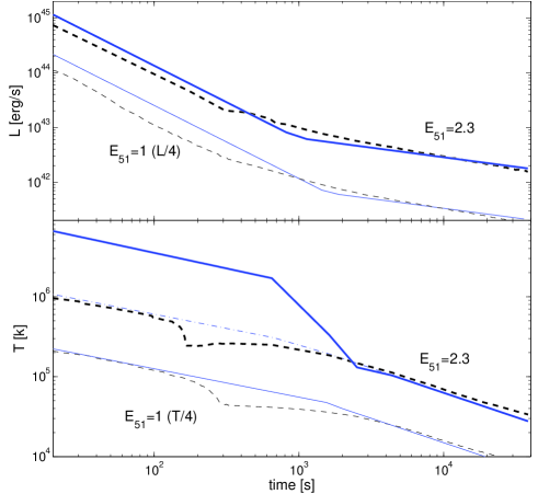
Figure 6: Bolometric luminosity (upper panel) and observed (color) temperature (lower panel) of two BSG explosions as a function of time, as obtained by the numerical simulation of Ensman & Burrows (1992) (dashed black line) and by our analytic calculation (solid blue line). The progenitor parameters are $M_{15}=16/15$ and $R_{50}=0.9$. The two explosions energies are $E_{51}=1$ (thin lines) and $E_{51}=2.3$ (thick lines). The luminosity and temperature of the $E_{51}=1$ explosion are divided by a factor of 4 (both ours and those obtained by Ensman & Burrows 1992). The temperature of the $E_{51}=2.3$ explosion in case that thermal equilibrium is artificially enforced is also plotted (thin dashed-dot line). See text for details.

Ensman & Burrows (1992) simulate several BSG explosions. They provide detailed luminosity and temperature curves, with no corrections for light travel time effects, of a BSG progenitor with $M_{*}=16~{}{\rm M}_{\odot}$ and $R_{*}=45~{}{\rm R}_{\odot}$ that explodes with energies of $10^{51}$ erg and $2.3\cdot 10^{51}$ erg. The temporal resolution is about $10$ s for the first few hundred seconds, adequate for comparison with BSG breakout and planar phase evolution. At later times they provide curves with a temporal resolution of about 0.5 hr. Ensman & Burrows (1992) allow for deviation of the gas temperature from the radiation temperatures and identify the color shell (i.e., thermalization depth) by the requirement $\sqrt{3\tau_{abs}\tau}=2/3$. They do however impose $\epsilon_{rad}=aT_{rad}^{4}$, where $\epsilon_{rad}$ and $T_{rad}$ are the radiation energy density and temperature respectively, thereby not allowing for deviation of the radiation from thermal equilibrium. Figure 6 shows the bolometric luminosity and observed temperature as functions of time obtained by Ensman & Burrows (1992). These are extracted from their figures 2 & 11 at early times and 3 & 12 at late times. $t=0$ is set such that the peak of the luminosity is at $t_{0}$. Figure 6 also shows our results of the luminosity and observed temperature. Our luminosity is calculated using equation 43 for both explosion energies. The excellent agreement between Ensman & Burrows (1992) numerical luminosity calculation and our analytic results is achieved without any fitting of the normalization or any other parameter. The results range over three orders of magnitude in time and luminosity and do not differ more than a factor of 2. The temporal decay slopes are similar and so are the values during the planar and spherical phases.

For $E_{51}=1$, the breakout thermal equilibrium is marginal ($\eta_{0}\approx 2$) and we plot only the temperature curve expected if thermal equilibrium is kept at all time (as enforce artificially by Ensman & Burrows 1992) using equation 38. For $E_{51}=2.3$, the breakout radiation is out of thermal equilibrium ($\eta_{0}\approx 13$) and therefore we calculate the temperature using equation 39. In order to compare our model to the results of Ensman & Burrows (1992) we also plot the temperature predicted in that case if there were thermal equilibrium at all time, using equation 38. The agreement between our model (when thermal equilibrium is enforced) and the results of Ensman & Burrows (1992) is very good. It is better than $20\%$ at any time, except for a period around a few hundred seconds where the temperatures of Ensman & Burrows (1992) drop over a short period by a factor of two. We do not see any physical origin for this behavior, which may be a numerical artifact. In the more energetic explosion, $E_{51}=2.3$, our model shows that the assumption of thermal equilibrium fails at early time and that Ensman & Burrows (1992) underestimate the breakout and planar phase observed temperature by an order of magnitude.

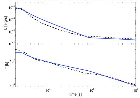
Figure 7: Bolometric luminosity (upper panel) and observed (color) temperature (lower panel) of an RSG explosion as function of time as obtained numerically by Tominaga et al. (2009) (dashed black line) and by our analytic calculation (solid blue line). The explosion parameters are $M_{15}=1.2$ and $R_{500}=1.6$ and $E_{51}=1.2$. The luminosity calculated by our analytic formula (equation 33) is deviled by a constant factor of 1.4. see text for details

Tominaga et al. (2009) simulate a $1.2\cdot 10^{51}$ erg explosion of an RSG progenitor with $M_{*}=18~{}{\rm M}_{\odot}$ and $R_{*}=800~{}{\rm R}_{\odot}$. They provide bolometric luminosity and observed temperature curves, where a travel time effects are included, assuming a spherical explosion. The temporal resolution is about $0.5$ hr for the first 14 hour and about 1 day at later times. We extract these curves from their figure 3 and set $t=0$ so the luminosity peaks at $t=R_{*}/c=1866$ s. Figure 7 shows the bolometric luminosity and observed temperature as functions of time obtained by Tominaga et al. (2009) and those obtained by our calculations. Our luminosity is calculated by using equation 33 and smoothing it for photon arrival time effect from a spherical explosion. The result is then divided by a constant factor of 1.4 to best fit the luminosity found by Tominaga et al. (2009). The similarity between the result of the detailed numerical simulation and our calculation is very good. Again, the luminosity ranges over three orders of magnitude and it is similar to within a factor of two at all times (factor of 3 if our luminosity is not divided by a constant factor of 1.4). The observed temperature is calculated using equation 35. At early times, when light travel time effects cause the observer to see a range of temperatures at any given moment, the maximal of these temperatures is taken. Our resulting temperature is not multiplied by any constant factor. The agreement between the numerical and analytic temperatures is again very good. It is similar at any time to within 30$\%$.

6 Summary

We derive analytic SNe light curves at early times, as long as recombination and radioactive decay do not play an important role. These light curves are valid while the observed temperature is above about $1$ eV and before injection by radioactive decay becomes important. These conditions hold during the first day after the explosion of a typical SN. The main advantage of our analysis over previous ones is the account for the radiation-gas coupling, which leads to determination of the observed temperature when the radiation at the color shell is out of thermal equilibrium. It also corrects previous estimates of the observed temperature, and the color shell location, when the radiation at the color shell is in thermal equilibrium. We define a thermal coupling coefficient, $\eta$, and find that the temperature evolution can follow two very different tracks, depending on $\eta_{0}$, i.e., the value of $\eta$ in the breakout shell at the breakout time. When the breakout shell is out of thermal equilibrium ($\eta_{0}>1$) the observed temperature starts high above the value obtained when thermal equilibrium is assumed and it drops faster than the case that the breakout shell is in thermal equilibrium. Thermal equilibrium is typically gained (when $\eta_{0}>1$) only at early stages of the spherical phase.

We discuss the luminosity and spetral evolution during the initial pulse and derive early SN light curves for various SN progenitors as a function of the explosion energy and the progenitor mass and radius. These are useful for interpretation of SNe light curves during the first day, which can teach us about properties of the progenitor star and potentially to lead to its identification. Additionally, it can be used to evaluate the effect of the early emission (e.g., ionization of the circum burst medium), in case that its detection is missed, on the environment at the SN vicinity. Finally it is useful for planning targeted searches of shock breakouts of various SNe types. The theory we discuss here can be also applied in some cases to shock breakout from non-SN stellar explosions. For example, the explosion of solar-like star by tidal forces in the vicinity of a super-massive black hole discussed recently by Guillochon et al. (2009).

The main conclusions based on our analysis are:

• It was shown that shock breakout radiation from WDs, WRs and some BSGs is out of thermal equilibrium (Katz, Budnik & Waxman, 2010). We show that it typically remains out of thermal equilibrium throughout the planar phase and until the early spherical phase. In SN from these compact progenitors the observed temperature at this time is significantly higher than the one obtained when thermal equilibrium is assumed. The observed temperature falls as $t^{-\alpha}$, where $1/3<\alpha<2/3$, during the planar phase, and once the evolution becomes spherical it plunges down (roughly as $t^{-2}$) until we observe radiation that is in thermal equilibrium at the source.

• Breakouts from RSGs and some BSGs are in thermal equilibrium. The flux at frequencies below $T_{obs}$ (e.g., optical/UV) starts with a bright initial pulse and then it decays during the planar phase reaching a minimum at $t_{s}$. The flux is rising during the planar phase reaching a second maximum when $T_{obs}$ falls into the observed frequency.

• In cases where the radiation is in thermal equilibrium at the source, the location of the thermalization depth, $r_{cl}$ is not trivial (e.g., Ensman & Burrows, 1992). The assumptions used in some previous analytic calculations, such as $r_{cl}=r(\tau=1)$ (e.g., Chevalier & Fransson, 2008) or $r_{cl}=\widehat{r}$ (e.g., Piro, Chang & Weinberg, 2009) are incorrect. Instead, in this case $\widehat{r}<r_{cl}<r(\tau=1)$ and it satisfies $r_{cl}=r({\eta=1})$, where $T_{obs}=(L\tau_{cl}/4\pi\sigma r_{cl}^{~{}2})^{1/4}$.

• The initial pulse, which is smeared by light travel-time and asphericity, contains emission from gas at different temperatures. The resulting combined spectrum is not a black-body. Instead, below the peak of $\nu F_{\nu}$ the spectrum is a power-law $F_{\nu}\propto\nu^{-\beta}$ where $0<\beta<1/2$. If asphericity is negligible then this effect is negligible in RSGs, minor in BSGs and significant in WRs, where a power-law $F_{\nu}\propto\nu^{-\beta}$, ranges over one or two orders of magnitude in $\nu$.

• The bolometric luminosity is dictated by the balance between the radiation diffusion time scale and the dynamical time scale (e.g., Chevalier, 1992). Namely, the source of the observed energy at any time is the shell where these two timescales are comparable. Since the photons dominate the heat capacity, the bolometric luminosity does not depend on the photon-gas coupling, and it evolves independently of the thermal coupling.

• The bolometric light curve and spectral evolution of the initial pulse depends on the explosion asphericity and wind transparency. A “bare” spherical explosion has a unique and therefore identifiable light curve. It shows multiple time scales as well as spectral evolution during the initial pulse. It rises quickly, over $t_{0}$, and lasts for $R_{*}/c$. A mildly opaque wind ($1<\tau_{w}<c/v_{0}$) results in a pulse of characteristic time $\tau_{w}R_{*}/c$ during which the spectrum does not evolve significantly. A “bare” aspherical explosion produces a time evolving spectrum, whose light curve and spectral evolution depends on the asphericity details. Much can be learned from observation of the initial pulse!

• The initial pulse of a RSG may release $\sim 3\cdot 10^{46}$ erg over a duration of $\sim 1000$ sec in soft X-rays $\approx 0.2$ keV. A BSG shock breakout releases a comparable amount of energy in harder X-rays over $\sim 100$ sec. The breakout from a WR releases $\sim 10^{45}$ erg within $\sim 10$ sec in the form of hard x-rays or soft $\gamma$-rays. Thus, not only WR stars, but also breakouts from BSGs and potentially RSGs are predicted to produce strong X-ray flares that can be detected by X-ray telescopes to large distances. WR breakouts may also be hard enough to be detectable by current soft gamma-ray detectors to a distance of $\sim 10$ Mpc, and mimic a single pulse long gamma-ray burst.

• The early emission from a type Ia SNe is in $\gamma$-rays. It is detectable within our galaxy by current detectors and may mimic a very short ($10-20$ ms) gamma-ray burst.

We thank Carlos Badenes, Orly Gnat, Chris Hirata, Amir Levinson, Tsvi Piran, Sterl Phinney and Amiel Sternberg for helpful discussions. E.N. was partially supported by the Israel Science Foundation (grant No. 174/08) and by an IRG grant. R.S. was partially supported by ERC and IRG grants, and a Packard Fellowships.

APPENDIX A- parameters of the breakout shell

Here we give a short list of values of various physical parameters of the breakout shell at the time of breakout. We consider three different progenitors of core collapse SNe - RSG (n=1.5, $\kappa=0.34{\rm~{}cm^{2}g^{-1}}$), BSG (n=3, $\kappa=0.34{\rm~{}cm^{2}g^{-1}}$) and WR (n=3, $\kappa=0.2{\rm~{}cm^{2}g^{-1}}$).

We approximate the density profile near the star surface as:

$$\rho\approx\rho_{*}\left(\frac{d_{i}}{R_{*}}\right)^{n}$$ (A -1)

where $\rho_{*}=M_{*}/R_{*}^{3}$. There is a correction factor of order unity to eq. A -1, which depends on the stellar structure, but the results are practically insensitive to this factor (Calzavara & Matzner, 2004). The properties at different locations near the stellar surface are

$$m=\frac{4\pi R_{*}^{3}\rho_{*}}{n+1}\left(\frac{\rho}{\rho_{*}}\right)^{\frac{n+1}{n}}$$ (A -2)

$$\tau=\frac{\kappa R_{*}\rho_{*}}{n+1}\left(\frac{\rho}{\rho_{*}}\right)^{\frac{n+1}{n}}$$ (A -3)

$$v=1800{\rm~{}km/s~{}}\left(\frac{E_{51}}{M_{15}}\right)^{1/2}\left(\frac{\rho}{\rho_{*}}\right)^{-0.19}$$ (A -4)

Note that we ignore the difference between the ejected mass (used ,e.g., by Matzner & McKee 1999) and the total stellar mass. The following properties of the breakout shell at the time of breakout are found by requiring $\tau=c/v_{0}$.

$$m_{0}\approx\left\{\begin{array}[]{c}10^{-3}~{}M_{\odot}~{}M_{15}^{0.43}R_{500}^{2.26}E_{51}^{-0.56}~{}~{}~{}~{}~{}{\rm(RSG)}\\ 3\cdot 10^{-6}~{}M_{\odot}~{}M_{15}^{0.41}R_{50}^{2.34}E_{51}^{-0.58}~{}~{}~{}~{}~{}{\rm(BSG)}\\ 3\cdot 10^{-8}~{}M_{\odot}~{}M_{15}^{0.41}R_{5}^{2.34}E_{51}^{-0.58}~{}~{}~{}~{}~{}{\rm(WR)}\end{array}\right.$$ (A -5)

$$\rho_{0}\approx\left\{\begin{array}[]{c}6\cdot 10^{-10}{\rm~{}g/cm^{3}~{}}M_{15}^{0.67}R_{500}^{-1.64}E_{51}^{-0.3}~{}~{}~{}~{}~{}{\rm(RSG)}\\ 2\cdot 10^{-9}{\rm~{}g/cm^{3}~{}}M_{15}^{0.56}R_{50}^{-1.25}E_{51}^{-0.44}~{}~{}~{}~{}~{}{\rm(BSG)}\\ 6\cdot 10^{-8}{\rm~{}g/cm^{3}~{}}M_{15}^{0.56}R_{5}^{-1.25}E_{51}^{-0.44}~{}~{}~{}~{}~{}{\rm(WR)}\end{array}\right.$$ (A -6)

$$v_{0}\approx\left\{\begin{array}[]{c}7000{\rm~{}km/s~{}}M_{15}^{-0.43}R_{500}^{-0.26}E_{51}^{0.56}~{}~{}~{}~{}~{}{\rm(RSG)}\\ 20,000{\rm~{}km/s~{}}M_{15}^{-0.41}R_{50}^{-0.33}E_{51}^{0.58}~{}~{}~{}~{}~{}{\rm(BSG)}\\ 40,000{\rm~{}km/s~{}}M_{15}^{-0.41}R_{5}^{-0.33}E_{51}^{0.58}~{}~{}~{}~{}~{}{\rm(WR)}\end{array}\right.$$ (A -7)

$$E_{0}\approx\left\{\begin{array}[]{c}9\cdot 10^{47}{\rm~{}erg~{}}M_{15}^{-0.43}R_{500}^{1.74}E_{51}^{0.56}~{}~{}~{}~{}~{}{\rm(RSG)}\\ 3\cdot 10^{46}{\rm~{}erg~{}}M_{15}^{-0.41}R_{50}^{1.66}E_{51}^{0.58}~{}~{}~{}~{}~{}{\rm(BSG)}\\ 9\cdot 10^{44}{\rm~{}erg~{}}M_{15}^{-0.41}R_{5}^{1.66}E_{51}^{0.58}~{}~{}~{}~{}~{}{\rm(WR)}\end{array}\right.$$ (A -8)

Note that $E_{0}$ is the internal energy in the breakout shell at $t_{0}$, while $E_{51}$ is the total explosion energy in units of $10^{51}$ erg.

$$\tau_{0}\approx\left\{\begin{array}[]{c}50~{}M_{15}^{0.43}R_{500}^{0.26}E_{51}^{-0.56}~{}~{}~{}~{}~{}{\rm(RSG)}\\ 15~{}M_{15}^{0.41}R_{50}^{0.33}E_{51}^{-0.58}~{}~{}~{}~{}~{}{\rm(BSG)}\\ 8~{}M_{15}^{0.41}R_{5}^{0.33}E_{51}^{-0.58}~{}~{}~{}~{}~{}{\rm(WR)}\end{array}\right.$$ (A -9)

$$\frac{d_{0}}{R_{*}}\approx\left\{\begin{array}[]{c}5.8\cdot 10^{-3}~{}M_{15}^{-0.22}R_{500}^{0.9}E_{51}^{-0.22}~{}~{}~{}~{}~{}{\rm(RSG)}\\ 6.1\cdot 10^{-3}~{}M_{15}^{-0.15}R_{50}^{0.58}E_{51}^{-0.15}~{}~{}~{}~{}~{}{\rm(BSG)}\\ 1.9\cdot 10^{-3}~{}M_{15}^{-0.15}R_{5}^{0.58}E_{51}^{-0.15}~{}~{}~{}~{}~{}{\rm(WR)}\end{array}\right.$$ (A -10)

$$t_{0}\approx\left\{\begin{array}[]{c}300{\rm~{}s~{}}M_{15}^{0.21}R_{500}^{2.16}E_{51}^{-0.79}~{}~{}~{}~{}~{}{\rm(RSG)}\\ 10{\rm~{}s~{}}M_{15}^{0.27}R_{50}^{1.91}E_{51}^{-0.73}~{}~{}~{}~{}~{}{\rm(BSG)}\\ 0.2{\rm~{}s~{}}M_{15}^{0.27}R_{5}^{1.91}E_{51}^{-0.73}~{}~{}~{}~{}~{}{\rm(WR)}\end{array}\right.$$ (A -11)

$$\frac{ct_{0}}{R_{*}}\approx\left\{\begin{array}[]{c}0.25~{}M_{15}^{0.21}R_{500}^{1.16}E_{51}^{-0.79}~{}~{}~{}~{}~{}{\rm(RSG)}\\ 0.09~{}M_{15}^{0.27}R_{50}^{0.91}E_{51}^{-0.73}~{}~{}~{}~{}~{}{\rm(BSG)}\\ 0.014~{}M_{15}^{0.27}R_{5}^{0.91}E_{51}^{-0.73}~{}~{}~{}~{}~{}{\rm(WR)}\end{array}\right.$$ (A -12)

$$t_{s}\approx\left\{\begin{array}[]{c}14{\rm~{}hr~{}}M_{15}^{0.43}R_{500}^{1.26}E_{51}^{-0.56}~{}~{}~{}~{}~{}{\rm(RSG)}\\ 0.5{\rm~{}hr~{}}M_{15}^{0.41}R_{50}^{1.33}E_{51}^{-0.58}~{}~{}~{}~{}~{}{\rm(BSG)}\\ 90{\rm~{}s~{}}M_{15}^{0.41}R_{5}^{1.33}E_{51}^{-0.58}~{}~{}~{}~{}~{}{\rm(WR)}\end{array}\right.$$ (A -13)

$$\eta_{0}\approx\left\{\begin{array}[]{c}0.06~{}M_{15}^{-1.72}R_{500}^{-0.76}E_{51}^{2.16}~{}~{}~{}~{}~{}{\rm(RSG)}\\ 2~{}M_{15}^{-1.63}R_{50}^{-1.1}E_{51}^{2.24}~{}~{}~{}~{}~{}{\rm(BSG)}\\ 24~{}M_{15}^{-1.63}R_{5}^{-1.1}E_{51}^{2.24}~{}~{}~{}~{}~{}{\rm(WR)}\end{array}\right.$$ (A -14)

$$T_{obs,0}\approx\left\{\begin{array}[]{lc}25{\rm~{}eV~{}}M_{15}^{-0.3}R_{500}^{-0.65}E_{51}^{0.5}&~{}~{}~{}~{}~{}{\rm(RSG)}\\ 80{\rm~{}eV~{}}M_{25}^{-0.28}R_{70}^{-0.62}E_{51}^{0.48}&~{}~{}~{}~{}~{}{\rm(BSG~{}thermal)}\\ 700{\rm~{}eV~{}}M_{10}^{-1.2}R_{20}^{-1.1}E_{51}^{1.7}&~{}~{}~{}~{}~{}{\rm(BSG~{}nonthermal)}\\ 2{\rm~{}keV~{}}M_{15}^{-1.7}R_{5}^{-1.5}E_{51}^{1.8}&~{}~{}~{}~{}~{}{\rm(WR)}\end{array}\right.$$ (A -15)

Note that $T_{obs,0}$ is the observed temperature at the time of breakout and not necessarily the temperature of the breakout shell at that time. The dependence of $T_{obs,0}$ in the nonthermal cases (BSG  nonthermal and WR) on $M_{*}$, $R_{*}$ and $E_{51}$ is approximated and calculated numerically. The reason is that the value of the logarithmic Comptonization factor $\xi$ has a non-power-law dependence on the explosion parameters. The power law indices we provide are accurate to within $\pm 0.5$ when $R_{*}$ and $M_{*}$ are larger or smaller by up to a factor of about 3, than our canonical values and $E_{51}=1-2$. In order to obtain a more accurate evaluation of nonthermal $T_{obs,0}$ when $M_{*}$, $R_{*}$ and $E_{51}$ differ from our canonical values, $7\rho_{0}$ (the factor of $7$ is due to the shock compression) should be plugged into equation 15 ($y_{max})$ and then equation 17 should be solved numerically (using $\eta_{0}$).

APPENDIX B - Electron-photon temperature coupling

Our temperature calculations (in particular equation 17) assume that in the relevant shells the electron temperature follows the photon temperature at all time. Here we examine the validity of this assumption.

Consider first a shell that is in thermal equilibrium at the time of breakout (i.e., $\eta_{i}<1$). As discussed in section 2.2.1 when $\eta<1$ a typical photon is absorbed at least once within the available time ($\min\{t,t_{d}\}$). Therefore, since photons dominate the energy density, the electron temperature is coupled to the radiation while $\eta<1$. Now, if in a shell $\eta_{i}<1$ then by the time that $\eta>1$ that shell does not affect the observed temperature anymore since at this point it is external to the luminosity shell. Therefore in such shells our temperature coupling coupling holds while relevant.

Next consider a shell that is initially out of thermal equilibrium (i.e., $\eta_{i}>1$). Here, absorbtion do not play a significant role and electrons follow the photons temperature if the rate at which they lose energy (electron cooling rate), mostly via free-free emission, is slower than the rate at which they gain energy via Compton scattering with typical photons (electron heating rate). The coupling in shells that are out of thermal equilibrium is important mostly during the planar phase, since during the spherical phase the color shell is quickly receding inward to shells that are in thermal equilibrium. Since during the planar phase only the breakout shell is observed (it is also the luminosity shell and the color shell when $\widehat{\eta}>1$) we consider only the coupling in this shell. Below we calculate the heating and cooling rates in the breakout shell that is out of thermal equilibrium during the planar phase.

The electron heating term is:

$$\dot{e}_{heat}=\frac{c}{l}\frac{n_{ph}}{n_{e}}\frac{3kT}{m_{e}c^{2}}3kT$$ (B-1)

where here we denote number densities as $n$ with different subscripts, not to be confused with the stellar envelope structure power-law index. $e$ is the energy of a single electron, $l=1/n_{e}\sigma_{T}$ is the photons mean free pass, $n_{ph}$ is the photon density, $n_{e}$ is the electron density and we take $3kT$ photons as responsible for most of the heating. Just behind the shock $n_{ph,i}\approx\frac{n_{u}m_{p}v_{0}^{2}}{kT_{i}}$ where $n_{u}$ is the upstream density (compressed by a factor of 7 in the shock, i.e., $n_{e,i}=7n_{u}$), implying:

$$\dot{e}_{heat}\approx c\sigma_{T}n_{e}\frac{m_{p}v^{2}}{m_{e}c^{2}}\frac{E}{E_{i}}kT$$ (B-2)

where $E$ is the total energy in the radiation and $E_{i}$ is its initial value. During the planar phase $E/E_{i}\propto t^{-1/3}$.

The main cooling process is free-free emission:

$$\dot{e}_{cool}\approx\alpha\sigma_{T}cn_{e}\sqrt{m_{e}c^{2}kT}$$ (B-3)

where $\alpha$ is the fine structure constant and we neglect the logarithmic factor $\xi$. We define the heating to cooling ratio:

$$\chi\equiv\frac{\dot{e}_{heat}}{\dot{e}_{cool}}\approx 4\left(\frac{v_{0}}{10^{4}~{}km/s}\right)^{2}\left(\frac{kT}{100~{}eV}\right)^{1/2}\left(\frac{t}{t_{0}}\right)^{-1/3}$$ (B-4)

If $\chi>1$ then electrons track the photons temperature, while if $\chi<1$ then Compton scattering is not enough to keep the electrons at the photons temperature. Thus, If $\chi<1$ and in addition $\eta>1$ in the breakout shell during the planar phase, then not Compton scattering nor free-free absorbtion can heat the electrons fast enough and our assumption of a single temperature fails. Using equations 18, 20 and $kT_{BB,0}\approx(v_{0}\rho_{0}/a)^{1/4}$ we find that while $\eta>1$ then in the breakout shell:

$$\chi\approx 5\eta^{8/5}\left(\frac{\rho_{0}}{10^{-10}~{}g/cm^{-3}}\right)^{1/5}\left(\frac{t}{t_{0}}\right)^{-2/5}.$$ (B-5)

Thus, our assumption of a single electron-photon temperature is valid during the breakout. Moreover, $\chi$ depends strongly on $\eta$ and only weakly on $t$ (e.g., in a typical BSG, $(t_{s}/t_{0})^{2/5}\approx 8$). Therefore, the request $\chi>1$ while $\eta>1$ may be at most marginally violated in the breakout shell during the planar phase, and only in a narrow range of the parameter phase space. Note that even if the electron temperature in the breakout shell decouples from that of the photons during the planar phase the modifications to the observed light curve are minor. The bolometric luminosity is of course not affected while the temperature in the breakout shell is not driven anymore towards thermal equilibrium and it starts dropping only via adiabatic cooling, e.g., $T_{obs}\propto t^{-1/3}$ (instead of a slightly faster decay). Later, the temperature evolution during the early spherical phase is also slightly modified. Nevertheless, the general behavior, that the temperature drops very sharply at $t_{s}<t$ until it approaches $\widehat{T}_{BB}$ and merges with the thermal equilibrium evolution at $t\approx t_{2}$, is unchanged.

Therefore, we conclude that our assumption that the electrons and photons temperatures are similar generally holds in the shells that determine the temperature evolution, and that even if it is violated over a small region of the relevant parameter phase space the modifications are small.

APPENDIX C - Glossary of main symbols and notations

• $t$: time since breakout

• $r$: radius

• $v$: velocity

• $m(r)$: mass at radius larger than $r$

• $\rho$: mass density

• $d$: shell width

• $\tau$: optical depth

• $E$: internal energy (not to be confused with $E_{51}$)

• $t_{d}$: diffusion time

• $\epsilon$: energy density

• $\eta$: Thermal coupling coefficient. Defined in equation 13

• $\xi$: logarithmic Comptonization term. Defined in equation 16

• $L$: observed luminosity

• $T_{obs}$: observed temperature (often denoted as color temperature). Defined as the typical photon energy.

• breakout shell: The shell where the shock breaks out (the shock width is comparable to the shell width).

• luminosity shell: The shell that generates the observed luminosity. In this shell the diffusion time equals to the dynamical time, t.

• color shell: The shell where the observed temperature is determined. This shell coincides with the thermalization depth when the observed radiation is in thermal equilibrium and with the luminosity shell when it is not.

• For any quantity $x$, we use the following subscripts and superscripts
  $x_{i}$: Initial value (after shock crossing) of a shell.
  $x_{0}$: value at the breakout shell at the time of breakout.
  $\widehat{x}$: value at the luminosity shell.
  $x_{cl}$: value at the color shell.

• $t_{0}$: Duration of shock breakout. Also, dynamical time, diffusion time, and shock crossing time of the breakout shell at the time of breakout.

• $t_{1}$: The first time where the observed temperature is in thermal equilibrium if it was not in thermal equilibrium from the beginning. Thermal equilibrium was achieved by photons produced at earlier time. Defined in equation 27

• $t_{2}$: The first time where the observed temperature is in thermal equilibrium, which is achieved by photons produced at $t_{2}$, if it was not in thermal equilibrium from the beginning. Defined in equation 29

• $t_{s}$: The transition time from planar to spherical geometry ($=R_{*}/v_{0}$).

• $T_{obs,0}$: observed temperature at $t_{0}$. Equal to the temperature of the breakout shell if it is out of thermal equilibrium. Otherwise it is lower than the breakout shell temperature.

• $T_{BB}$: Thermal equilibrium temperature appropriate for a given energy density by Boltzmann’s law. Defined in equation 12.

• $R_{*}$: stelar radius

• $M_{*}$: stelar mass

• $E_{51}$: explosion energy in units of $10^{51}$ erg

• $n$: power-law index describing the pre-explosion stellar density profile near the edge.

References

- Blinnikov et al. (1998) Blinnikov, S. I., Eastman, R., Bartunov, O. S., Popolitov, V. A., and Woosley, S. E. 1998, ApJ, 496, 454, arXiv:astro-ph/9711055.
- Calzavara & Matzner (2004) Calzavara, A. J. and Matzner, C. D. 2004, MNRAS, 351, 694, arXiv:astro-ph/0312464.
- Campana et al. (2006) Campana, S. et al. 2006, Nature, 442, 1008, arXiv:astro-ph/0603279.
- Chevalier (1976) Chevalier, R. A. 1976, ApJ, 207, 872.
- Chevalier (1992) Chevalier, R. A. 1992, ApJ, 394, 599.
- Chevalier & Fransson (2008) Chevalier, R. A. and Fransson, C. 2008, ApJ, 683, L135.
- Colgate (1974) Colgate, S. A. 1974, ApJ, 187, 333.
- Couch et al. (2010) Couch, S. M., Pooley, D., Wheeler, J. C., and Milosavljevic, M. 2010, ArXiv e-prints, 1007.3693.
- Ensman & Burrows (1992) Ensman, L. and Burrows, A. 1992, ApJ, 393, 742.
- Falk (1978) Falk, S. W. 1978, ApJ, 225, L133.
- Freytag et al. (2002) Freytag, B., Steffen, M., & Dorch, B. 2002, Astronomische Nachrichten, 323, 213
- Gezari et al. (2008) Gezari, S. et al. 2008, ApJ, 683, L131, 0804.1123.
- Grassberg, Imshennik & Nadyozhin (1971) Grassberg, E. K., Imshennik, V. S., and Nadyozhin, D. K. 1971, Ap&SS, 10, 28.
- Guillochon et al. (2009) Guillochon, J., Ramirez-Ruiz, E., Rosswog, S., and Kasen, D. 2009, ApJ, 705, 844, arXiv:astro-ph/0811.1370.
- Imshennik & Nadezhin (1988) Imshennik, V. S. and Nadezhin, D. K. 1988, Soviet Astronomy Letters, 14, 449.
- Imshennik, Nadezhin & Utrobin (1981) Imshennik, V. S., Nadezhin, D. K., and Utrobin, V. P. 1981, Ap&SS, 78, 105.
- Katz, Budnik & Waxman (2010) Katz, B., Budnik, R., and Waxman, E. 2010, ApJ, 716, 781, arXiv:astro-ph/0902.4708.
- Klein & Chevalier (1978) Klein, R. I. and Chevalier, R. A. 1978, ApJ, 223, L109.
- Li (2007) Li, L. 2007, MNRAS, 375, 240, arXiv:astro-ph/0605387.
- Matzner & McKee (1999) Matzner, C. D. and McKee, C. F. 1999, ApJ, 510, 379, arXiv:astro-ph/9807046.
- Modjaz et al. (2009) Modjaz, M. et al. 2009, ApJ, 702, 226, arXiv:astro-ph/0805.2201.
- Piro, Chang & Weinberg (2009) Piro, A. L., Chang, P., and Weinberg, N. N. 2009, ArXiv e-prints, 0909.2643.
- Rabinak & Waxman (2010) Rabinak, I. and Waxman, E. 2010, ArXiv e-prints, arXiv:astro-ph/1002.3414.
- Sakurai (1960) Sakurai, A. 1960, Communications on Pure and Applied Mathematics, 13, 353.
- Schawinski et al. (2008) Schawinski, K. et al. 2008, Science, 321, 223, arXiv:astro-ph/0803.3596.
- Schwarzschild (1958) Schwarzschild, M. 1958, Structure and evolution of the stars., ).
- Shigeyama, Nomoto & Hashimoto (1988) Shigeyama, T., Nomoto, K., and Hashimoto, M. 1988, A&A, 196, 141.
- Soderberg et al. (2008) Soderberg, A. M. et al. 2008, Nature, 453, 469, arXiv:astro-ph/0802.1712.
- Svensson (1984) Svensson, R. 1984, MNRAS, 209, 175.
- Tan, Matzner & McKee (2001) Tan, J. C., Matzner, C. D., and McKee, C. F. 2001, ApJ, 551, 946, arXiv:astro-ph/0012003.
- Tominaga et al. (2009) Tominaga, N., Blinnikov, S., Baklanov, P., Morokuma, T., Nomoto, K., and Suzuki, T. 2009, ApJ, 705, L10, arXiv:astro-ph/0908.2162.
- Waxman, Mészáros & Campana (2007) Waxman, E., Mészáros, P., and Campana, S. 2007, ApJ, 667, 351, arXiv:astro-ph/0702450.
- Weaver (1976) Weaver, T. A. 1976, ApJS, 32, 233.
- Weaver et al. (1978) Weaver, T. A., Zimmerman, G. B., & Woosley, S. E. 1978, ApJ, 225, 1021
- Woosley (1988) Woosley, S. E. 1988, ApJ, 330, 218.