The uncertainty principle determines the non-locality of quantum mechanics

Two central concepts of quantum mechanics are Heisenberg’s uncertainty principle, and a subtle form of non-locality that Einstein famously called “spooky action at a distance”. These two fundamental features have thus far been distinct concepts. Here we show that they are inextricably and quantitatively linked. Quantum mechanics cannot be more non-local with measurements that respect the uncertainty principle. In fact, the link between uncertainty and non-locality holds for all physical theories. More specifically, the degree of non-locality of any theory is determined by two factors – the strength of the uncertainty principle, and the strength of a property called “steering”, which determines which states can be prepared at one location given a measurement at another.

A measurement allows us to gain information about the state of a physical system. For example when measuring the position of a particle, the measurement outcomes correspond to possible locations. Whenever the state of the system is such that we can predict this position with certainty, then there is only one measurement outcome that can occur. Heisenberg [16] observed that quantum mechanics imposes strict restrictions on what we can hope to learn – there are incompatible measurements such as position and momentum whose results cannot be simultaneously predicted with certainty. These restrictions are known as uncertainty relations. For example, uncertainty relations tell us that if we were able to predict the momentum of a particle with certainty, then when measuring its position all measurement outcomes occur with equal probability. That is, we are completely uncertain about its location.

Non-locality can be exhibited when performing measurements on two or more distant quantum systems – the outcomes can be correlated in way that defies any local classical description [6]. This is why we know that quantum theory will never by superceded by a local classical theory. Nevertheless, even quantum correlations are restricted to some extent – measurement results cannot be correlated so strongly that they would allow signalling between two distant systems. However quantum correlations are still weaker than what the no-signalling principle demands [26, 27, 28]. So, why are quantum correlations strong enough to be non-local, yet not as strong as they could be? Is there a principle that determines the degree of this non-locality? Information-theory [33, 24], communication complexity [38], and local quantum mechanics [3] provided us with some rationale why limits on quantum theory may exist. But evidence suggests that many of these attempts provide only partial answers. Here, we take a very different approach and relate the limitations of non-local correlations to two inherent properties of any physical theory.

Uncertainty relations

At the heart of quantum mechanics lies Heisenberg’s uncertainty principle [16]. Traditionally, uncertainty relations have been expressed in terms of commutators

$$\Delta A\Delta B\geq\ \frac{1}{2}|\langle\psi|[A,B]|\psi\rangle|.$$ (1)

with standard deviations $\Delta X=\sqrt{\langle\psi|X^{2}|\psi\rangle-\langle\psi|X|\psi\rangle^{2}}$ for $X\in\{A,B\}$. However, the more modern approach is to use entropic measures. Let $p(x^{(t)}|t)_{\sigma}$ denote the probability that we obtain outcome $x^{(t)}$ when performing a measurement labelled $t$ when the system is prepared in the state $\sigma$. In quantum theory, $\sigma$ is a density operator, while for a general physical theory, we assume that $\sigma$ is simply an abstract representation of a state. The well-known Shannon entropy $H(t)_{\sigma}$ of the distribution over measurement outcomes of measurement $t$ on a system in state $\sigma$ is thus

$$H(t)_{\sigma}:=-\sum_{x^{(t)}}p(x^{(t)}|t)_{\sigma}\log p(x^{(t)}|t)_{\sigma}\ .$$ (2)

In any uncertainty relation, we wish to compare outcome distributions for multiple measurements. In terms of entropies such relations are of the form

$$\sum_{t\in\mathcal{T}}p(t)\ H(t)_{\sigma} \geq c_{\mathcal{T},{\mathcal{D}}},$$ (3)

where $p(t)$ is any probability distribution over the set of measurements $\mathcal{T}$, and $c_{\mathcal{T},{\mathcal{D}}}$ is some positive constant determined by $\mathcal{T}$ and the distribution ${\mathcal{D}}=\{p(t)\}_{t}$. To see why (3) forms an uncertainty relation, note that whenever $c_{\mathcal{T},{\mathcal{D}}}>0$ we cannot predict the outcome of at least one of the measurements $t$ with certainty, i.e., $H(t)_{\sigma}>0$. Such relations have the great advantage that the lower bound $c_{\mathcal{T},{\mathcal{D}}}$ does not depend on the state $\sigma$ [12]. Instead, $c_{\mathcal{T},{\mathcal{D}}}$ depends only on the measurements and hence quantifies their inherent incompatibility. It has been shown that for two measurements, entropic uncertainty relations do in fact imply Heisenberg’s uncertainty relation [7], providing us with a more general way of capturing uncertainty (see [42] for a survey).

One may consider many entropic measures instead of the Shannon entropy. For example, the min-entropy

$$H_{\infty}(t)_{\sigma}:=-\log\max_{x^{(t)}}p(x^{(t)}|t)_{\sigma}\$$ (4)

used in [12], plays an important role in cryptography and provides a lower bound on $H(t)_{\sigma}$. Entropic functions are, however, a rather coarse way of measuring the uncertainty of a set of measurements, as they do not distinguish the uncertainty inherent in obtaining any combination of outcomes $x^{(t)}$ for different measurements $t$. It is thus useful to consider much more fine-grained uncertainty relations consisting of a series of inequalities, one for each combination of possible outcomes, which we write as a string ${\vec{x}}=(x^{(1)},\ldots,x^{(n)})\in\mathcal{B}^{\times n}$ with $n=|\mathcal{T}|$ . That is, for each ${\vec{x}}$, a set of measurements $\mathcal{T}$, and distribution ${\mathcal{D}}=\{p(t)\}_{t}$,

$$P^{\rm cert}(\sigma;{\vec{x}}):=\sum_{t=1}^{n}p(t)\ p(x^{(t)}|t)_{\sigma}\leq\zeta_{\vec{x}}(\mathcal{T},{\mathcal{D}})\ .$$ (5)

For a fixed set of measurements, the set of inequalities

$$\mathcal{U}=\left\{\sum_{t=1}^{n}p(t)\ p(x^{(t)}|t)_{\sigma}\ \leq\zeta_{\vec{x}}\mid\forall{\vec{x}}\in\mathcal{B}^{\times n}\right\}\ ,$$ (6)

thus forms a fine-grained uncertainty relation, as it dictates that one cannot obtain a measurement outcome with certainty for all measurements simultaneously whenever $\zeta_{\vec{x}}<1$. The values of $\zeta_{\vec{x}}$ thus confine the set of allowed probability distributions, and the measurements have uncertainty if $\zeta_{\vec{x}}<1$ for all ${\vec{x}}$. To characterise the “amount of uncertainty” in a particular physical theory, we are thus interested in the values of

$$\zeta_{\vec{x}}=\max_{\sigma}\sum_{t=1}^{n}p(t)p(x^{(t)}|t)_{\sigma}\$$ (7)

where the maximization is taken over all states allowed on a particular system (for simplicity, we assume it can be attained in the theory considered). We will also refer to the state $\rho_{{\vec{x}}}$ that attains the maximum as a “maximally certain state”. However, we will also be interested in the degree of uncertainty exhibited by measurements on a set of states $\Sigma$ quantified by $\zeta_{\vec{x}}^{\Sigma}$ defined with the maximisation in Eq. 7 taken over ${\sigma\in\Sigma}$. Fine-grained uncertainty relations are directly related to the entropic ones, and have both a physical and an information processing appeal (see appendix). As an example, consider the binary spin-$1/2$ observables $Z$ and $X$. If we can obtain a particular outcome $x^{(Z)}$ given that we measured $Z$ with certainty i.e. $p(x^{(Z)}|Z)=1$, then the complementary observable must be completely uncertain i.e. $p(x^{(X)}|X)=1/2$. If we choose which measurement to make with probability $1/2$ then this notion of uncertainty is captured by the relations

$$\frac{1}{2}p(x^{(X)}|X)+\frac{1}{2}p(x^{(Z)}|Z)\leq\zeta_{\vec{x}}=\frac{1}{2}+\frac{1}{2\sqrt{2}}\mbox{ for all }{\vec{x}}=(x^{(X)},x^{(Z)})\in\{0,1\}^{2}\ ,$$ (8)

where the maximally certain states are given by the eigenstates of $(X+Z)/\sqrt{2}$ and $(X-Z)/\sqrt{2}$.

Non-local correlations

We now introduce the concept of non-local correlations. Instead of considering measurements on a single system we consider measurements on two (or more) space-like separated systems traditionally named Alice and Bob. We label Bob’s measurements using $t\in\mathcal{T}$, and use $b\in\mathcal{B}$ to label his measurement outcomes. For Alice, we use $s\in\mathcal{S}$ to label her measurements, and $a\in\mathcal{A}$ to label her outcomes (recall, that wlog we can assume all measurements have the same number of outcomes). When Alice and Bob perform measurements on a shared state $\sigma_{AB}$ the outcomes of their measurements can be correlated. Let $p(a,b|s,t)_{\sigma_{AB}}$ be the joint probability that they obtain outcomes $a$ and $b$ for measurements $s$ and $t$. We can now again ask ourselves, what correlations are possible in nature? In other words, what probability distributions are allowed?

Quantum mechanics as well as classical mechanics obeys the no-signalling principle, meaning that information cannot travel faster than light. This means that the probability that Bob obtains outcome $b$ when performing measurement $t$ cannot depend on which measurement Alice chooses to perform (and vice versa). More formally, $\sum_{a}p(a,b|s,t)_{\sigma_{AB}}=p(b|t)_{\sigma_{B}}$ for all $s$, where $\sigma_{B}=\mathop{\mathsf{tr}}\nolimits_{A}(\sigma_{AB})$. Curiously, however, this is not the only constraint imposed by quantum mechanics [26], and finding other constraints is a difficult task [21, 14]. Here, we find that the uncertainty principle imposes the other limitation.

To do so, let us recall the concept of so-called Bell inequalities [6], which are used to describe limits on such joint probability distributions. These are most easily explained in their more modern form in terms of a game played between Alice and Bob. Let us choose questions $s\in\mathcal{S}$ and $t\in\mathcal{T}$ according to some distribution $p(s,t)$ and send them to Alice and Bob respectively, where we take for simplicity $p(s,t)=p(s)p(t)$. The two players now return answers $a\in\mathcal{A}$ and $b\in\mathcal{B}$. Every game comes with a set of rules that determines whether $a$ and $b$ are winning answers given questions $s$ and $t$. Again for simplicity, we thereby assume that for every $s$,$t$ and $a$, there exists exactly one winning answer $b$ for Bob (and similarly for Alice). That is, for every setting $s$ and outcome $a$ of Alice there is a string ${\vec{x}_{s,a}}=({x_{s,a}}^{(1)},\ldots,{x_{s,a}}^{(n)})\in\mathcal{B}^{\times n}$ of length $n=|\mathcal{T}|$ that determines the correct answer $b={x_{s,a}}^{(t)}$ for question $t$ for Bob (Fig. 1). We say that $s$ and $a$ determine a “random access coding” [40], meaning that Bob is not trying to learn the full string ${\vec{x}_{s,a}}$ but only the value of one entry. The case of non-unique games is a straightforward but cumbersome generalisation.

As an example, the Clauser-Horne-Shimony-Holt (CHSH) inequality [11], one of the simplest Bell inequalities whose violation implies non-locality, can be expressed as a game in which Alice and Bob receive binary questions $s,t\in\{0,1\}$ respectively, and similarly their answers $a,b\in\{0,1\}$ are single bits. Alice and Bob win the CHSH game if their answers satisfy $a\oplus b=s\cdot t$. We can label Alice’s outcomes using string ${\vec{x}_{s,a}}$ and Bob’s goal is to retrieve the $t$-th element of this string. For $s=0$, Bob will always need to give the same answer as Alice in order to win and hence we have $\vec{x}_{0,0}=(0,0)$, and $\vec{x}_{0,1}=(1,1)$. For $s=1$, Bob needs to give the same answer for $t=0$, but the opposite answer if $t=1$. That is, $\vec{x}_{1,0}=(0,1)$, and $\vec{x}_{1,1}=(1,0)$.

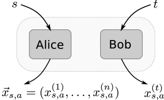
Figure 1: Any game where for every choice of settings $s$ and $t$, and answer $a$ of Alice, there is only one correct answer $b$ for Bob can be expressed using strings ${\vec{x}_{s,a}}$ such that $b={x_{s,a}}^{(t)}$ is the correct answer for Bob [40] for $s$ and $a$. The game is equivalent to Alice outputting ${\vec{x}_{s,a}}$ and Bob outputting ${x_{s,a}}^{(t)}$.

Alice and Bob may agree on any strategy ahead of time, but once the game starts their physical distance prevents them from communicating. For any physical theory, such a strategy consists of a choice of shared state $\sigma_{AB}$, as well as measurements, where we may without loss of generality assume that the players perform a measurement depending on the question they receive and return the outcome of said measurement as their answer. For any particular strategy, we may hence write the probability that Alice and Bob win the game as

$${P^{\rm game}(\mathcal{S},\mathcal{T},\sigma_{AB})}=\sum_{s,t}p(s,t)\sum_{a}p(a,b={x_{s,a}}^{(t)}|s,t)_{\sigma_{AB}}$$ (9)

To characterize what distributions are allowed, we are generally interested in the winning probability maximized over all possible strategies for Alice and Bob

$${P^{\rm game}_{\rm max}}=\max_{\mathcal{S},\mathcal{T},\sigma_{AB}}{P^{\rm game}(\mathcal{S},\mathcal{T},\sigma_{AB})}\ ,$$ (10)

which in the case of quantum theory, we refer to as a Tsirelson’s type bound for the game [35]. For the CHSH inequality, we have ${P^{\rm game}_{\rm max}}=3/4$ classically, ${P^{\rm game}_{\rm max}}=1/2+1(2\sqrt{2})$ quantum mechanically, and ${P^{\rm game}_{\rm max}}=1$ for a theory allowing any nonsignalling correlations. ${P^{\rm game}_{\rm max}}$ quantifies the strength of nonlocality for any theory, with the understanding that a theory possesses genuine nonlocality when it differs from the value that can be achieved classically. The connection we will demonstrate between uncertainty relations and nonlocality holds even before this optimization.

Steering

The final concept, we need in our discussion is steerability, which determines what states Alice can prepare on Bob’s system remotely. Imagine Alice and Bob share a state $\sigma_{AB}$, and consider the reduced state $\sigma_{B}=\mathop{\mathsf{tr}}\nolimits_{A}(\sigma_{AB})$ on Bob’s side. In quantum mechanics, as well as many other theories in which Bob’s state space is a convex set $\mathscr{S}$, the state $\sigma_{B}\in\mathscr{S}$ can be decomposed in many different ways as a convex sum

$$\sigma_{B}=\sum_{a}p(a|s)\ \sigma_{s,a}\mbox{ with }\sigma_{s,a}\in\mathscr{S}\ ,$$ (11)

corresponding to an ensemble $\mathcal{E}_{s}=\{p(a|s),\sigma_{s,a}\}_{a}$. It was Schrödinger [30, 31] who noted that in quantum mechanics for all $s$ there exists a measurement on Alice’s system that allows her to prepare $\mathcal{E}_{s}=\{p(a|s),\sigma_{s,a}\}_{a}$ on Bob’s site (Fig. 2). That is for measurement $s$, Bob’s system will be in the state $\sigma_{s,a}$ with probability $p(a|s)$. Schrödinger called this steering to the ensemble $\mathcal{E}_{s}$ and it does not violate the no-signalling principle, because for each of Alice’s setting, the state of Bob’s system is the same once we average over Alice’s measurement outcomes.

Even more, he observed that for any set of ensembles $\{\mathcal{E}_{s}\}_{s}$ that respect the no-signalling constraint, i.e., for which there exists a state $\sigma_{B}$ such that Eq. 11 holds, we can in fact find a bipartite quantum state $\sigma_{AB}$ and measurements that allow Alice to steer to such ensembles.

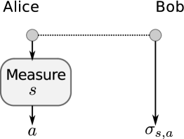
Figure 2: When Alice performs a measurement labelled $s$, and obtains outcome $a$ with probability $p(a|s)$ she effectively prepares the state $\sigma_{s,a}$ on Bob’s system. This is known as “steering”.

We can imagine theories in which our ability to steer is either more, or maybe even less restricted (some amount of signalling is permitted). Our notion of steering thus allows forms of steering not considered in quantum mechanics [30, 31, 43, 18] or other restricted classes of theories [4]. Our ability to steer, however, is a property of the set of ensembles we consider, and not a property of one single ensemble.

Main result

We are now in a position to derive the relation between how non-local a theory is, and how uncertain it is. For any theory, we will find that the uncertainty relation for Bob’s measurements (optimal or otherwise) acting on the states that Alice can steer to is what determines the strength of non-locality (See Eq. (14)). We then find that in quantum mechanics, for all games where the optimal measurements are known, the states which Alice can steer to are identical to the most certain states, and it is thus only the uncertainty relations of Bob’s measurements which determine the outcome (see Eq. (15)).

First of all, note that we may express the probability (9) that Alice and Bob win the game using a particular strategy (Fig 1) as

$${P^{\rm game}(\mathcal{S},\mathcal{T},\sigma_{AB})}=\sum_{s}p(s)\sum_{a}p(a|s)P^{\rm cert}(\sigma_{s,a};{\vec{x}_{s,a}})\ ,$$ (12)

where $\sigma_{s,a}$ is the reduced state of Bob’s system for setting $s$ and outcome $a$ of Alice, and $p(t)$ in $P^{\rm cert}(\cdot)$ is the probability distribution over Bob’s questions $\mathcal{T}$ in the game. This immediately suggests that there is indeed a close connection between games and our fine-grained uncertainty relations. In particular, every game can be understood as giving rise to a set of uncertainty relations and vice versa. It is also clear from Eq. 5 for Bob’s choice of measurements $\mathcal{T}$ and distribution ${\mathcal{D}}$ over $\mathcal{T}$ that the strength of the uncertainty relations imposes an upper bound on the winning probability

$${P^{\rm game}(\mathcal{S},\mathcal{T},\sigma_{AB})} \leq\sum_{s}p(s)\sum_{a}p(a|s)\ \zeta_{{\vec{x}_{s,a}}}(\mathcal{T},{\mathcal{D}})\leq\max_{{\vec{x}_{s,a}}}\zeta_{{\vec{x}_{s,a}}}(\mathcal{T},{\mathcal{D}})\ ,$$ (13)

where we have made explicit the functional dependence of $\zeta_{\vec{x}}$ on the set of measurements. This seems curious given that we know from [44] that any two incompatible observables lead to a violation of the CHSH inequality, and that to achieve Tsirelson’s bound Bob has to measure maximally incompatible observables [25] that yield stringent uncertainty relations. However, from Eq. 13 we may be tempted to conclude that for any theory it would be in Bob’s best interest to perform measurements that are very compatible and have weak uncertainty relations in the sense that the values $\zeta_{{\vec{x}_{s,a}}}$ can be very large. But, can Alice prepare states $\sigma_{s,a}$ that attain $\zeta_{{\vec{x}_{s,a}}}$ for any choice of Bob’s measurements?

The other important ingredient in understanding non-local games is thus steerability. We can think of Alice’s part of the strategy $\mathcal{S},\sigma_{AB}$ as preparing the ensemble $\{p(a|s),\sigma_{s,a}\}_{a}$ on Bob’s system, whenever she receives question $s$. Thus when considering the optimal strategy for non-local games, we want to maximise ${P^{\rm game}(\mathcal{S},\mathcal{T},\sigma_{AB})}$ over all ensembles $\mathcal{E}_{s}=\{p(a|s),\sigma_{s,a}\}_{a}$ that Alice can steer to, and use the optimal measurements $\mathcal{T}_{\rm opt}$ for Bob. That is,

$${P^{\rm game}_{\rm max}}=\max_{\{\mathcal{E}_{s}\}_{s}}\sum_{s}p(s)\sum_{a}p(a|s)\ \zeta_{\vec{x}}^{\sigma_{s,a}}(\mathcal{T}_{\rm opt},{\mathcal{D}})\ ,$$ (14)

and hence the probability that Alice and Bob win the game depends only on the strength of the uncertainty relations with respect to the sets of steerable states. To achieve the upper bound given by Eq. 13 Alice needs to be able to prepare the ensemble $\{p(a|s),\rho_{{\vec{x}_{s,a}}}\}_{a}$ of maximally certain states on Bob’s system. In general, it is not clear that the maximally certain states for the measurements which are optimal for Bob in the game can be steered to.

It turns out that in quantum mechanics, this can be achieved in cases where we know the optimal strategy. For all XOR games , that is correlation inequalities for two outcome observables (which include CHSH as a special case), as well as other games where the optimal measurements are known we find that the states which are maximally certain can be steered to (see appendix). The uncertainty relations for Bob’s optimal measurements thus give a tight bound

$${P^{\rm game}_{\rm max}}=\sum_{s}p(s)\sum_{a}p(a|s)\zeta_{\vec{x}}(\mathcal{T}_{\rm opt},{\mathcal{D}})\ ,$$ (15)

where we recall that $\zeta_{\vec{x}}$ is the bound given by the maximization over the full set of allowed states on Bob’s system. It is an open question whether this holds for all games in quantum mechanics.

An important consequence of this is that any theory that allows Alice and Bob to win with a probability exceeding ${P^{\rm game}_{\rm max}}$ requires measurements which do not respect the fine-grained uncertainty relations given by $\zeta_{\vec{x}}$ for the measurements used by Bob (the same argument can be made for Alice). Even more, it can lead to a violation of the corresponding min-entropic uncertainty relations (see appendix). For example, if quantum mechanics were to violate the Tsirelson bound using the same measurements for Bob, it would need to violate the min-entropic uncertainty relations [12]. This relation holds even if Alice and Bob were to perform altogether different measurements when winning the game with a probability exceeding ${P^{\rm game}_{\rm max}}$: for these new measurements there exist analogous uncertainty relations on the set $\Sigma$ of steerable states, and a higher winning probability thus always leads to a violation of such an uncertainty relation. Conversely, if a theory allows any states violating even one of these fine-grained uncertainty relations for Bob’s (or Alice’s) optimal measurements on the sets of steerable states, then Alice and Bob are able to violate the Tsirelson’s type bound for the game.

Although the connection between non-locality and uncertainty is more general, we examine the example of the CHSH inequality in detail to gain some intuition on how uncertainty relations of various theories determine the extent to which the theory can violate Tsirelson’s bound (see appendix). To briefly summerize, in quantum theory, Bob’s optimal measurements are $X$ and $Z$ which have uncertainty relations given by $\zeta_{\vec{x}_{s,a}}=1/2+1/(2\sqrt{2})$ of Eq. 8. Thus, if Alice could steer to the maximally certain states for these measurements, they would be able to achieve a winning probability given by ${P^{\rm game}_{\rm max}}=\zeta_{\vec{x}_{s,a}}$ i.e. the degree of non-locality would be determined by the uncertainty relation. This is the case – if Alice and Bob share the singlet state then Alice can steer to the maximally certain states by measuring in the basis given by the eigenstates of $(X+Z)/\sqrt{2}$ or of $(X-Z)/\sqrt{2}$. For quantum mechanics, our ability to steer is only limited by the no-signalling principle, but we encounter strong uncertainty relations.

On the other hand, for a local hidden variable theory, we can also have perfect steering, but only with an uncertainty relation given by $\zeta_{\vec{x}_{s,a}}=3/4$, and thus we also have the degree of non-locality given by ${P^{\rm game}_{\rm max}}=3/4$. This value of non-locality is the same as deterministic classical mechanics where we have no uncertainty relations on the full set of deterministic states, but our abilities to steer to them are severely limited. In the other direction, there are theories that are maximally non-local, yet remain no-signalling [26]. These have no uncertainty, i.e. $\zeta_{\vec{x}_{s,a}}=1$, but unlike in the classical world we still have perfect steering, so they win the CHSH game with probability $1$.

For any physical theory we can thus consider the strength of non-local correlations to be a tradeoff between two aspects: steerability and uncertainty. In turn, the strength of non-locality can determine the strength of uncertainty in measurements. However, it does not determine the strength of complementarity of measurements (see appendix). The concepts of uncertainty and complementarity are usually linked, but we find that one can have theories that are just as non-local and uncertain as quantum mechanics, but that have less complementarity. This suggests a rich structure relating these quantities, which may be elucidated by further research in the direction suggested here.

Acknowledgments The retrieval game used was discovered in collaboration with Andrew Doherty. JO is supported by the Royal Society. SW is supported by NSF grants PHY-04056720 and PHY-0803371, the National Research Foundation and the Ministry of Education, Singapore. Part of this work was done while JO was visiting Caltech (Pasadena, USA), and while JO and SW were visiting KITP (Santa Barbara, USA) funded by NSF grant PHY-0551164.

Supplementary Material

In this appendix we provide the technical details used or discussed in the main part. In Section A we show that for the case of XOR games, Alice can always steer to the maximally certain states of Bob’s optimal measurement operators. That is, the relation between uncertainty relations and non-local games does not depend on any additional steering constraints. Hence, a violation of the Tsirelson’s bound implies a violation of the corresponding uncertainty relation. Conversely, a violation of the uncertainty relation leads to a violation of the Tsirelson bound as long the theory allows Alice to steer to the new maximally certain states. The famous CHSH game is a particular example of an XOR game, and in Sections A.3 and B we find that Tsirelson’s bound [35] is violated if and only if Deutsch’ min-entropic uncertainty relation [12] is violated, whenever steering is possible. In fact, for an even wider class of games called retrieval games a violation of Tsirelson’s bound implies a violation of the min-entropic uncertainty relations for Bob’s optimal measurement derived in [41].

In Section B we show that our fine-grained uncertainty relations are not only directly related to entropic uncertainty relations

$$\sum_{t=1}^{n}H_{\infty}(t)_{\sigma}\geq-\log\max_{{\vec{x}}}\zeta_{\vec{x}}\ ,$$ (16)

but they are particularly appealing from both a physical, as well as an information processing perspective: For measurements in a full set of so-called mutually unbiased bases, the $\zeta_{\vec{x}}$ are the extrema of the discrete Wigner function used in physics [45]. From an information processing perspective, we may think of the string ${\vec{x}}$ as being encoded into quantum states $\sigma_{{\vec{x}}}$ where we can perform the measurement $t$ to retrieve the $t$-th entry from ${\vec{x}}$. Such an encoding is known as a random access encoding of the string ${\vec{x}}$ [2, 23]. The value of $\zeta_{\vec{x}}$ can now be understood as an upper bound on the probability that we retrieve the desired entry correctly, averaged over our choice of $t$ which is just $P^{\rm cert}(\sigma_{{\vec{x}}})$. This upper bound is attained by the maximally certain state $\rho_{\vec{x}}$. Bounds on the performance of random access encodings thus translate directly into uncertainty relations and vice versa.

In Section C we discuss a number of example theories in the context of CHSH in order to demonstrate the interplay between uncertainty and non-locality. This includes quantum mechanics, classical mechanics, local hidden variable models and theories which are maximally non-local but still non-signalling. In Section D, we show that although non-locality might determine the extent to which measurements in a theory are uncertain, it does not determine how complementary the measurements are. We distinguish these concepts and give an example in the case of the CHSH inequality, of a theory which is just as non-local and uncertain as quantum mechanics, but where the measurements are less complementary. Finally, in Section E we show how the form of any uncertainty relation can be used to construct a non-local game.

Appendix A XOR-games

In this section, we concentrate on showing that for the case of XOR-games, the relation between uncertainty relations and non-local games does not involve steering constraints, since the steering is only limited by the no-signalling condition. Quantum mechanics allows Alice to steer Bob’s states to those which are maximally certain for his optimal measurement settings. For quantum mechanics to become more non-local, it must have weaker uncertainty relations for steerable states.

First of all, let us recall some important facts about XOR games. These games are equivalent to Bell inequalities for observables with two outcomes i.e. bipartite correlation inequalities for dichotomic observables. They form the only general class of games which are truly understood at present. Not only do we know the structure of the measurements that Alice and Bob will perform, but we can also find them efficiently using semidefinite programming for any XOR game [39], which remains a daunting problem for general games [14, 21, 22].

A.1 Structure of measurements

We first recall the structure of the optimal measurements used by Alice and Bob. In an XOR game, the answers $a\in\{0,1\}$ and $b\in\{0,1\}$ of Alice and Bob respectively are single bits, and the decision whether Alice and Bob win or not depends only on the XOR of the answers $a\oplus b=a+b\mod 2$. The winning condition can thus be written in terms of a predicate that obeys $V(c=a\oplus b|s,t)=1$ if and only if $a\oplus b=c$ are winning answers for Alice and Bob given settings $s$ and $t$ (otherwise $V(c|s,t)=0$). Let $A_{s}^{a}$ and $B_{t}^{b}$ denote the measurement operators corresponding to measurement settings $s$ and $t$ giving outcomes $a$ and $b$ of Alice and Bob respectively. Without loss of generality, we may thereby assume that these are projective measurements satisfying $A_{s}^{a}A_{s}^{a^{\prime}}=\delta_{a,a^{\prime}}A_{s}^{a}$, and similarly for Bob. Since we have only two measurement outcomes, we may view this measurement as measuring the observables

$$A_{s} =A_{s}^{0}-A_{s}^{1}\ ,$$ (17)

$$B_{t} =B_{t}^{0}-B_{t}^{1}\ ,$$ (18)

with outcomes $\pm 1$ where we label the outcome ’$+1$’ as ’$0$’, and the outcome ’$-1$’ as ’$1$’. Tsirelson [35, 36] has shown that the optimal winning probability for Alice and Bob can be achieved using traceless observables of the form

$$A_{s} =\sum_{j}a_{s}^{(j)}\Gamma_{j}\ ,$$ (19)

$$B_{t} =\sum_{j}b_{t}^{(j)}\Gamma_{j}\ ,$$ (20)

where $\vec{a}_{s}=(a_{s}^{(1)},\ldots,a_{s}^{(N)})\in\mathbb{R}^{N}$ and $\vec{b}_{t}=(b_{t}^{(1)},\ldots,b_{t}^{(N)})\in\mathbb{R}^{N}$ are real unit vectors of dimension $N=\min(|\mathcal{S}|,|\mathcal{T}|)$ and $\Gamma_{1},\ldots,\Gamma_{N}$ are the anti-commuting generators of a Clifford algebra. That is, we have

$$\{\Gamma_{j},\Gamma_{k}\} =\Gamma_{j}\Gamma_{k}+\Gamma_{k}\Gamma_{j}=0\mbox{ for all }j\neq k\ ,$$ (21)

$$(\Gamma_{j})^{2} =\mathbb{I}\mbox{ for all }j$$ (22)

In dimension $d=2^{n}$ we can find at most $N=2n+1$ such operators, which can be obtained using the well known Jordan-Wigner transform [19]. Since we have $A_{s}^{0}+A_{s}^{1}=\mathbb{I}$ and $B_{t}^{0}+B_{t}^{1}=\mathbb{I}$ we may now use Eqs. 17 and 18 to express the measurement operators in terms of the observables as

$$A_{s}^{a} =\frac{1}{2}\left(\mathbb{I}+(-1)^{a}A_{s}\right)\ ,$$ (23)

$$B_{t}^{b} =\frac{1}{2}\left(\mathbb{I}+(-1)^{b}B_{t}\right)\ .$$ (24)

Tsirelson furthermore showed that the optimal state that Alice and Bob use with said observables is the maximally entangled state

$$|\psi\rangle=\frac{1}{\sqrt{d}}\sum_{k=0}^{d-1}|k\rangle|k\rangle$$ (25)

of total dimension $d=(2^{\lfloor{N/2}\rfloor})^{2}$.

To see how XOR games are related to Bell correlation inequalities note that we may use Eqs. 23 and 24 to rewrite the winning probability of the game in terms of the observables as

$${P^{\rm game}(\mathcal{S},\mathcal{T},\sigma_{AB})} =\sum_{s,t}p(s,t)\sum_{a,b}V(a,b|s,t)\langle\psi|A_{s}^{a}\otimes B_{t}^{b}|\psi\rangle$$ (26)

$$=\frac{1}{2}\left(\sum_{s,t}p(s,t)\sum_{c}V(c|s,t)\left(1+(-1)^{c}\langle\psi|A_{s}\otimes B_{t}|\psi\rangle\right)\right)\ .$$ (27)

For example, for the well known CHSH inequality given by

$$\langle\psi|CHSH|\psi\rangle =\langle\psi|A_{0}\otimes B_{0}+A_{0}\otimes B_{1}+A_{1}\otimes B_{0}-A_{1}\otimes B_{1}|\psi\rangle\$$ (28)

with $p(s,t)=p(s)p(t)=1/4$ we have

$${P^{\rm game}(\mathcal{S},\mathcal{T},\sigma_{AB})} =\frac{1}{2}\left(1+\frac{\langle\psi|CHSH|\psi\rangle}{4}\right)$$ (29)

$$=\frac{1}{4}\sum_{s,t}\sum_{a,b}V(a,b|s,t)\langle\psi|A_{s}^{a}\otimes B_{t}^{b}|\psi\rangle\ ,$$ (30)

where $V(a,b|s,t)=1$ if and only if $a\oplus b=s\cdot t$.

A.2 Steering to the maximally certain states

Now that we know the structure of the measurements that achieve the maximal winning probability in an XOR game, we can write down the corresponding uncertainty operators for Bob (the case for Alice is analogous). Once we have done that, we will see that it is possible for Alice to steer Bob’s state to the maximally certain ones. First of all, note that in the quantum case we have that the set of measurement operators $\{B_{t}\}_{t}$ is each decomposable in terms of POVM elements $\{B_{t}^{b}\}_{b}$, and thus $\zeta_{\vec{x}}$ corresponds to the largest eigenvalue of the uncertainty operator

$$Q_{{\vec{x}_{s,a}}}=\sum_{t}p(t)B_{t}^{x_{s,a}^{(t)}}\ .$$ (31)

The $Q$ are positive operators, so sets of them, together with an error operator form a positive valued operator and can be measured. In the case of XOR games, we thus have

$$Q_{{\vec{x}_{s,a}}}=\sum_{t}p(t)\sum_{\begin{subarray}{c}b\\ V(a,b|s,t)=1\end{subarray}}B_{t}^{b}\ ,$$ (32)

and the Bell polynomial can be expressed as

$$\beta =\sum_{stab}p(s)p(t)V(ab|st)A_{s}^{a}\otimes B_{t}^{b}$$ (33)

$$=\sum_{sa}p(s)A_{s}^{a}\otimes Q_{{\vec{x}_{s,a}}}\ .$$ (34)

For the special case of XOR-games we can now use Eq. 24 to rewrite Bob’s uncertainty operator using the short hand $\vec{v}\cdot\vec{\Gamma}=\sum_{j}v^{(j)}\Gamma_{j}$ as

$$Q_{{\vec{x}_{s,a}}} =\frac{1}{2}\sum_{t}p(t)\sum_{\begin{subarray}{c}b\\ V(a,b|s,t)=1\end{subarray}}\left(\mathbb{I}+(-1)^{b}B_{t}\right)$$

$$=\frac{1}{2}\left[c_{s,a}\mathbb{I}+\vec{v}_{s,a}\cdot\vec{\Gamma}\right]\ ,$$ (35)

where

$$c_{s,a} =\sum_{t}p(t)|\sum_{b}V(a,b|s,t)|\,$$ (36)

$$\vec{v}_{s,a} =\sum_{t}p(t)\sum_{\begin{subarray}{c}b\\ V(a,b|s,t)=1\end{subarray}}(-1)^{b}\ \vec{b}_{t}$$ (37)

What makes XOR games so appealing, is that we can now easily compute the maximally certain states. Except for the case of two measurements, and rank one measurement operators this is generally not so easy to do, even though bounds may of course be found. Finding a general expression for such maximally certainty states allows us easily to compute the extrema of the discrete Wigner function as well as to prove tight entropic uncertainty relations for all measurements. This has been an open problem since Deutsch’s initial bound for two measurements using rank one operators [12, 42]. In particular, we recall for completeness [15] that

Claim A.1.

For any XOR game, we have that for any uncertainty operator $Q_{{\vec{x}_{s,a}}}$ of observables of the form Eqs. 19 and 20

$$\zeta_{\vec{x}_{s,a}}=\max_{\begin{subarray}{c}\rho\geq 0\\ \mathop{\mathsf{tr}}\nolimits{\rho}=1\end{subarray}}\mathop{\mathsf{tr}}\nolimits\left(\rho Q_{{\vec{x}_{s,a}}}\right)=\mathop{\mathsf{tr}}\nolimits(\rho_{{\vec{x}_{s,a}}}Q_{{\vec{x}_{s,a}}})=\frac{1}{2}\left(c_{s,a}+\|\vec{v}_{s,a}\|_{2}\right)$$ (38)

with

$$\rho_{{\vec{x}_{s,a}}}=\frac{1}{d}\left(\mathbb{I}+\sum_{j}r_{s,a}^{(j)}\Gamma_{j}\right)$$ (39)

and

$$\vec{r}_{s,a}=\vec{v}_{s,a}/\|\vec{v}_{s,a}\|_{2}\ .$$ (40)

Proof.

We first note that the set of operators $\{\mathbb{I}\}\cup\{\Gamma_{j}\}_{j}\cup\{i\Gamma_{j}\Gamma_{k}\}_{jk}\cup\ldots$ forms an orthonormal  basis for $d\times d$ Hermitian operators [13]. We may hence write any state $\rho$ as

$$\rho=\frac{1}{d}\left(\mathbb{I}+\sum_{j}r^{(j)}_{s,a}\Gamma_{j}+\ldots\right)\ ,$$ (41)

for some real coefficients $r^{(j)}_{s,a}$. Using the fact that $\mathcal{S}$ forms an orthonormal basis, we then obtain from Eq. 35 that

$$\mathop{\mathsf{tr}}\nolimits(\rho Q_{{\vec{x}_{s,a}}})=\frac{1}{2}\left(c_{s,a}+\vec{r}_{s,a}\cdot\vec{v}_{s,a}\right)\ .$$ (42)

Since for any quantum state $\rho$ we must have $\|\vec{r}_{s,a}\|_{2}\leq 1$ [41], maximising the left hand side corresponds to maximising the right hand side over vectors $\vec{r}_{s,a}$ of unit length. The claim now follows by noting that if $\vec{r}_{s,a}$ has unit length, then $\rho_{{\vec{x}_{s,a}}}$ is also a valid quantum state [41]. ∎

Note that the states $\rho_{{\vec{x}_{s,a}}}$ are highly mixed outside of dimension $d=2$, but still correspond to the maximally certain states. We now claim that that for any setting $s$, Alice can in fact steer to the states which are optimal for Bob’s uncertainty operator.

Lemma A.2.

For any XOR game we have for all $s,\hat{s}\in\mathcal{S}$

$$\sum_{a}p(a|s)\ \rho_{{\vec{x}_{s,a}}}=\sum_{a}p(a|\hat{s})\ \rho_{\hat{s},a}\ ,$$ (43)

where $\rho_{{\vec{x}_{s,a}}}$ is defined as in Eq. 39.

Proof.

First of all, note that it is easy to see in any XOR game the marginals of Alice (and analogously, Bob) are uniform. That is, the probability that Alice obtains outcome $a$ given setting $s$ obeys

$$p(a|s) =\langle\psi|A_{s}^{a}\otimes\mathbb{I}|\psi\rangle$$ (44)

$$=\frac{1}{2}\left(\langle\psi|\mathbb{I}\otimes\mathbb{I}|\psi\rangle+(-1)^{a}\langle\psi|A_{s}\otimes\mathbb{I}|\psi\rangle\right)$$

$$=\frac{1}{2}\left(1+\mathop{\mathsf{tr}}\nolimits(A_{s}^{T})\right)=\frac{1}{2}\ .$$

Second, it follows from the fact that we are considering an XOR game that $\vec{v}_{s,a}=-\vec{v}_{s,1-a}$ for all $s$ and $a$. Hence, by Claim A.1 we have $\vec{r}_{s,a}=-\vec{r}_{s,1-a}$ and hence

$$\frac{1}{2}\left(\rho_{{\vec{x}_{s,0}}}+\rho_{{\vec{x}_{s,1}}}\right)=\frac{\mathbb{I}}{d}\ ,$$ (45)

from which the statement follows. ∎

Unrelated to our problem, it is interesting to note that the observables $A_{s}=\vec{a}_{s}\cdot\vec{\Gamma}$ employed by Alice are determined exactly by the vectors $r_{s,a}$ above. Let $\sigma_{a,s}$ denote Bob’s post-measurement state which are steered to when Alice performs the measurement labelled by $s$ and obtains outcome $a$. We then have that for any of Bob’s measurement operators

$$\mathop{\mathsf{tr}}\nolimits\left(\sigma_{s,a}Q_{{\vec{x}_{s,a}}}\right) =\frac{\langle\psi|A_{s}^{a}\otimes Q_{{\vec{x}_{s,a}}}|\psi\rangle}{p(a|s)}$$ (46)

$$=\frac{1}{2}\left(c_{s,a}+(-1)^{a}\vec{a}_{s}\cdot\vec{v}_{s,a}\right)\ .$$ (47)

Since Alice’s observables should obey $(A_{s})^{2}=\mathbb{I}$, we would like that $\|\vec{a}_{s}\|_{2}=1$. When trying to find the optimal measurements for Alice we are hence faced with exactly the same task as when trying to optimize over states $\rho_{{\vec{x}_{s,a}}}$ in Claim A.1. That is, letting $\vec{a}_{s}=(-1)^{a}r_{s,a}$ gives us the optimal observables for Alice.

A.3 Retrieval games and entropic uncertainty relations

As a further example, we now consider a special class of non-local games that we call a retrieval games, which are a class of XOR games. This class includes the famous CHSH game. Retrieval games have the further property, that not only are the fine-grained uncertainty relations violated if quantum mechanics would be more non-local, but also the min-entropic uncertainty relation derived in [41] would be violated. The class of retrieval games are those which correspond directly to the retrieval of a bit from an $n$-bit string More precisely, we label the settings of Alice using all the $n$-bit strings starting with a ’0’. That is,

$$\mathcal{S}=\{(0,s^{(2)},\ldots,s^{(n)})\mid s^{(j)}\in\{0,1\}\}\ ,$$ (48)

where we will choose each setting with uniform probability $p(s)=1/2^{n-1}$. For each setting $s$, Alice has two outcomes which we label using the strings $s$ and $\underline{s}$, where $\underline{s}$ is the bitwise complement of the string $s$. More specifically, we let

$${\vec{x}}_{s,0} =s\ ,$$ (49)

$${\vec{x}}_{s,1} =\underline{{\it{s}}}\ .$$ (50)

Bob’s settings are labelled by the indices $\mathcal{T}=\{1,\ldots,n\}$, and chosen uniformly at random $p(t)=1/n$. Alice and Bob win the game if and only if Bob outputs the bit at position $t$ of the string that Alice outputs. In terms of the predicate, the game rules can be written as

$$V(a,b|s,t)=\left\{\begin{array}[]{cc}1&\mbox{ if }b={\vec{x}}_{s,a}^{(t)}\ ,\\ 0&\mbox{ otherwise}\ .\end{array}\right.$$ (53)

We call such a game a retrieval game of length $n$. It is not hard to see that the CHSH game above is a retrieval game of length $n=2$ [40].

We now show that for the case of retrieval games, not only can Alice steer perfectly to the optimal uncertainty states, but Bob’s optimal measurements are in fact very incompatible in the sense that his measurement operators necessarily anti-commute. In particular, this means that we obtain very strong uncertainty relations for Bob’s optimal measurements [41], as we will discuss in more detail below.

Lemma A.3.

Let $B_{t}=B_{t}^{0}-B_{t}^{1}$ denote Bob’s optimal dichotomic observables in dimension $d=2^{n}$. Then for any retrieval game

$$\{B_{t},B_{t^{\prime}}\}=0\mbox{ for all }t\neq t^{\prime}\in\mathcal{T}\ .$$ (54)

Proof.

First of all note that using Claim A.1 we can write the winning probability for arbitrary observables $B_{t}=\vec{b}_{t}\cdot\vec{\Gamma}$ in terms of the maximum uncertainty states $\rho_{{\vec{x}_{s,a}}}$ as

$${P^{\rm game}(\mathcal{S},\mathcal{T},\sigma_{AB})} =\frac{1}{2^{n}}\sum_{s,a}\mathop{\mathsf{tr}}\nolimits\left(\rho_{{\vec{x}_{s,a}}}Q_{{\vec{x}_{s,a}}}\right)$$ (55)

$$=\frac{1}{2^{n}}\sum_{s,a}\frac{1}{2}\left(1+\|\vec{v}_{s,a}\|_{2}\right)$$ (56)

$$=\frac{1}{2}\left(1+\frac{1}{2^{n}}\sum_{s,a}\sqrt{\vec{v}_{s,a}\cdot\vec{v}_{s,a}}\right)$$ (57)

$$\leq\frac{1}{2}\left(1+\sqrt{\frac{1}{2^{n}}\sum_{s,a}\sum_{tt^{\prime}}(-1)^{{\vec{x}}_{s,a}^{(t)}}(-1)^{{\vec{x}}_{s,a}^{(t^{\prime})}}\vec{b}_{t}\cdot\vec{b}_{t^{\prime}}}\right)$$ (58)

$$=\frac{1}{2}+\frac{1}{2\sqrt{n}}\ ,$$ (59)

where the inequality follows from the concavity of the square-root function and Jensen’s inequality, and the final inequality from the fact that $\vec{b}_{t}$ is of unit length. Equality with this upper bound can be achieved by choosing $\vec{b}_{t}\cdot\vec{b}_{t^{\prime}}=0$ for all $t\neq t^{\prime}$, which is equivalent to $\{B_{t},B_{t^{\prime}}\}=0$ for all $t\neq t^{\prime}$. ∎

For our discussions about uncertainty relations in the next section, it will be useful to note that the above implies that $\lambda_{\rm max}(Q_{{\vec{x}_{s,a}}})=\lambda_{\rm max}(Q_{{\vec{x}_{s^{\prime},a^{\prime}}}})$ for all settings $s,s^{\prime}\in\mathcal{S}$ and outcomes $a,a^{\prime}\in\mathcal{A}$. A useful consequence of the fact that $\vec{b}_{t}\cdot\vec{b}_{t^{\prime}}=0$ for $t\neq t^{\prime}$ is also that the probability that Bob retrieves a bit of the string ${\vec{x}_{s,a}}$ correctly is the same for all bits:

Corollary A.4.

For a retrieval game, we have for the optimal strategy that for all settings $s\in\mathcal{S}$ and outcomes $a\in\mathcal{A}$

$$\mathop{\mathsf{tr}}\nolimits\left(\rho_{{\vec{x}_{s,a}}}B_{t}^{{\vec{x}}_{s,a}^{(t)}}\right)=\mathop{\mathsf{tr}}\nolimits\left(\rho_{{\vec{x}_{s,a}}}B_{t^{\prime}}^{{\vec{x}}_{s,a}^{(t^{\prime})}}\right)\mbox{ for all }t,t^{\prime}\in\mathcal{T}\ .$$ (60)

The fact that min-entropic uncertainty relations are violated if quantum mechanics were to do better than the Tsirelson’s bound for retrieval games will be shown in Section B.

It is an interesting open question, whether Alice can steer to the maximally certain states for Bob’s optimal measurements for all games. This is for example possible, for the $\mod 3$-game suggested in [10] to which the optimal measurements were derived in [17, 20]. Unfortunately, the structure of measurement operators that are optimal for Bob is ill-understood for most games, which makes this a more difficult task.

Appendix B Min-entropic uncertainty relations

We now discuss the relationship between fine-grained uncertainty relations and min-entropic ones. The relation between retrieval games and min-entropic uncertainty relations will follow from that. Recall that the min-entropy of the distribution obtained by measuring a state $\rho$ using the measurement given by the observables $B_{t}$ can be written as

$$H_{\infty}(B_{t})_{\rho}=-\log\max_{x^{(t)}\in\{0,1\}}\mathop{\mathsf{tr}}\nolimits(B_{t}^{x^{(t)}}\rho)\ .$$ (61)

A min-entropic uncertainty relation for the measurements in an $n$-bit retrieval game can be bounded as

$$\frac{1}{n}\sum_{t=1}^{n}H_{\infty}(B_{t})_{\rho} =-\frac{1}{n}\sum_{t}\log\max_{x^{(t)}\in\{0,1\}}\mathop{\mathsf{tr}}\nolimits\left(B_{t}^{x^{(t)}}\rho\right)$$ (62)

$$\geq-\log\max_{\vec{\tilde{x}}\in\mathcal{B}^{\times n}}\sum_{t}\mathop{\mathsf{tr}}\nolimits\left(B_{t}^{\tilde{x}^{(t)}}\rho\right)$$ (63)

$$=-\log\max_{s,a}\lambda_{\rm max}(Q_{{\vec{x}_{s,a}}})\ ,$$ (64)

where the inequality follows from Jensen’s inequality and the concavity of the log. I.e. the fine-grained relations provide a lower bound on the min-entropic uncertainty relations.

Now we note that for the case of retrieval games, not only do we have

$$\lambda_{\rm max}(Q_{{\vec{x}_{s,a}}})=\frac{1}{2}+\frac{1}{2\sqrt{n}}\ ,$$ (65)

but by Corollary A.4 we have that the inequality 63 is in fact tight, where equality is achieved for any of the maximum uncertainty states $\rho_{{\vec{x}_{s,a}}}$ from the retrieval game. We thus have

Theorem B.1.

For any retrieval game, a violation of the Tsirelson’s bound implies a violation of the min-entropic uncertainty relations for Bob’s optimal measurements. A violation of the min-entropic uncertainty relation implies a violation of the Tsirelson’s bound as long as steering is possible.

Note that since the CHSH game is a retrieval game with $n=2$, we have that as long as steering is possible, Tsirelson’s bound [35] is violated if and only if Deutsch’ min-entropic uncertainty relation [12] is violated for Bob’s (or Alice’s) measurements.

Appendix C An example: the CHSH inequality in general theories

Probably the most well studied Bell inequality is the CHSH inequality and previous attempts to understand the strength of quantum non-locality have been with respect to it [24, 38, 9, 1]. Although the connections between non-locality and uncertainty are more general, we can use the CHSH inequality as an example and show how the uncertainty relations of various theories determine the extent to which the theory can violate it. We will see in this example how non-locality requires steering (which is what prevents classical mechanics from violating a Bell inequality despite having maximal certainty). Furthermore, we will see that local-hidden variable theories can have increased steering ability, but don’t violate a Bell inequality because they exactly compensate by having more uncertainty. Quantum mechanics has perfect steering, and so it’s non-locality is limited only by the uncertainty principle. We will also discuss theories which have the same degree of steering as quantum theory, but greater non-locality because they have greater certainty (so-called “PR-boxes” [26, 27, 28] being an example).

The CHSH inequality can be expressed as a game in which Alice and Bob receive binary questions $s,t\in\{0,1\}$ respectively, and similarly their answers $a,b\in\{0,1\}$ are single bits. Alice and Bob win the CHSH game if their answers satisfy $a\oplus b=s\cdot t$. The CHSH game thus belongs to the class of XOR games, and any other XOR game could be used as a similar example.

Note that we may again rephrase the game in the language of random access coding [40], where we label Alice’s outcomes using string ${\vec{x}_{s,a}}$ and Bob’s goal is to retrieve the $t$-th element of this string. For $s=0$, Bob will always need to give the same answer as Alice in order to win independent of $t$, and hence we have $\vec{x}_{0,0}=(0,0)$, and $\vec{x}_{0,1}=(1,1)$. For $s=1$, Bob needs to give the same answer for $t=0$, but the opposite answer if $t=1$. That is, $\vec{x}_{1,0}=(0,1)$, and $\vec{x}_{1,1}=(1,0)$.

To gain some intuition of the tradeoff between steerability and uncertainty, we consider an (over)simplified example in Figure 3. We examine quantum, classical, and a theory allowing maximal non-locality below.

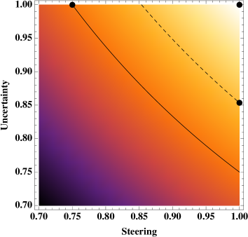
Figure 3: A simplified example: Imagine a world in which the only steerable states are the maximally certain states of the uncertainty relations we consider, and we have an all or nothing form of steering. I.e., either Alice can steer to all ensembles with probability $p_{\rm steer}$, or fails entirely. The vertical axis denotes the certainty $p_{\rm cert}$ (that is, the lack of uncertainty), and the horizontal axis $p_{\rm steer}$. Lighter colours indicate a larger winning probability, which in this simplified case is just ${P^{\rm game}(\mathcal{S},\mathcal{T},\sigma_{AB})}=p_{\rm steer}p_{\rm cert}$. The solid line denotes the case of ${P^{\rm game}_{\rm max}}=3/4$, which can be achieved classically. The point on the line denotes the combination of values for a classical deterministic theory: there is no uncertainty ($\zeta_{{\vec{x}_{s,a}}}=1$ for all ${\vec{x}_{s,a}}$), and no steering other than the trivial one to the state Alice and Bob already share as part of their strategy which yields $3/4$ on average. The dashed line denotes the value ${P^{\rm game}_{\rm max}}=1/2+1/(2\sqrt{2})$ achievable by a quantum strategy. The point on the line denotes the point reached quantumly: there is uncertainty, but we can steer perfectly to the maximally certain states. Finally, the point at $(1,1)$ denotes the point achievable by “PR-boxes”: there is no uncertainty, but nevertheless perfect steering.

(i) Quantum mechanics:

As we showed in Section A we have for any XOR game that we can always steer to the maximally certain states $\rho_{{\vec{x}_{s,a}}}$, and hence Alice’s and Bob’s winning probability depend only on the uncertainty relations. For CHSH, Bob’s optimal measurement are given by the binary observables $B_{0}=Z$ and $B_{1}=X$. The amount of uncertainty we observe for Bob’s optimal measurements is given by

$$\zeta_{\vec{x}_{s,a}}=\frac{1}{2}+\frac{1}{2\sqrt{2}}\mbox{ for all }{\vec{x}_{s,a}}\in\{0,1\}^{2}\ ,$$ (66)

where the maximally certain states are given by the eigenstates of $(X+Z)/\sqrt{2}$ and $(X-Z)/\sqrt{2}$. Alice can steer Bob’s states to the eigenstates of these operators by measuring in the basis of these operators on the state

$$|\psi^{-}\rangle=\frac{1}{\sqrt{2}}(|00\rangle_{AB}+|11\rangle_{AB})\ .$$ (67)

We hence have ${P^{\rm game}_{\rm max}}=\zeta_{\vec{x}_{s,a}}=1/2+1/(2\sqrt{2})$ which is Tsirelson’s bound [35, 36]. If Alice and Bob could obtain a higher value for the same measurements, at least one of the fine-grained uncertainty relations is violated. We also saw above that a larger violation for CHSH also implies a violation of Deutsch’ min-entropic uncertainty relation.

(ii) Classical mechanics & local hidden variable theories:

For classical theories, let us first consider the case where we use a deterministic strategy, since classically there is no fundamental restriction on how much information can be gained i.e., if we optimize the uncertainty relations over all classical states, we have $\zeta_{\vec{x}_{s,a}}=1$ for any set of measurements. However, for the states which are maximally certain, there is no steering property either because in the no-signalling constraint the density matrix has only one term in it. A deterministic state cannot be written as a convex sum of any other states – it is an extremal point of a convex set. The best deterministic strategy is thus to prepare a particular state at Bob’s site (e.g. an encoding of the bit-string $00$). This results in ${P^{\rm game}(\mathcal{S},\mathcal{T},\sigma_{AB})}=3/4$. A probabilistic strategy cannot do better, since it would be a convex combination of deterministic strategies and one might as well choose the best one. However, it will be instructive to consider the non-deterministic case.

Although the maximally certain states cannot be steered to, we can steer to states which are mixtures of deterministic states (c.f. [32]). This corresponds to using a non-deterministic strategy, or if the non-determinism is fundamental, to a local hidden variable theory. However, measurements on the states which can be steered to will not have well-defined outcomes. If we optimize the uncertainty relations with respect to the non-deterministic states, we will find that there is a substantial uncertainty in measurement outcomes on these states. We will find that the ability to steer is exactly compensated by an inability to obtain certain measurement outcomes, thus the probability of winning the non-local game will again be ${P^{\rm game}(\mathcal{S},\mathcal{T},\sigma_{AB})}=3/4$.

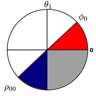
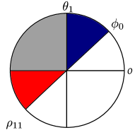
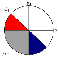
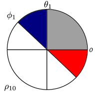
Figure 4: The hidden variable states $\rho_{{\vec{x}}}$ which encode each of the four random access strings on Bob’s site are depicted above. The grey region corresponds to the hidden variable being such that Bob can correctly retrieve both bits. The blue and red regions correspond to the region where Bob incorrectly retrieves the first or second bit respectively. These regions must be included if Alice is to be able to steer to the states.

Figure 4 depicts an optimal local hidden variable theory for CHSH where the local hidden variable is a point on the unit circle labelled by an angle $\Omega$ and the states are probability distributions

$$\rho_{{\vec{x}_{s,a}}}=\int_{\Omega_{{\vec{x}_{s,a}}}}^{\Omega_{{\vec{x}_{s,a}}}^{\prime}}p(\Omega)\sigma_{\Omega}d\Omega$$ (68)

with $\sigma_{\Omega}$ denoting the state of the hidden variable, and $p(\Omega)$ uniform. Alice can prepare these states at Bob’s site if they initially share the maximally correlated state $\psi^{MC}_{AB}=\int_{0}^{2\pi}p(\Omega)\sigma^{\Omega}_{A}\sigma^{\Omega}_{B}d\Omega$ and she makes a partial measurement on her state which determines that the value of her hidden variable lies within $\Omega_{{\vec{x}_{s,a}}}$ and $\Omega_{{\vec{x}_{s,a}}}^{\prime}$.

A measurement by Bob corresponds to cutting the circle in half along some angle, and then determining whether the hidden variable lies above or below the cut. I.e. a coarse grained determination of the bounds of integration in $\rho_{{\vec{x}_{s,a}}}$ to within $\pi$. Bob’s measurement for $t=0$ thereby corresponds to determining whether the hidden variable lies above or below the cut along the equator, while his measurement for $t=1$ corresponds to determining whether the hidden variable lies above or below the cut labelled by the angle $\theta_{1}$. If the hidden variable is above the cut, we label the outcome as $1$, and $0$ otherwise.

First of all, note that if the hidden variable lies in the region shaded in grey, as depicted in Figure 4, then Bob will be able to retrieve both bits correctly because it lies in the region such that the results for Bob’s measurements would match the string that the state encodes. For example, for the $\rho_{00}$ state, the hidden variable in the grey region lies below both cuts, while for the $\rho_{11}$ state, the hidden variable lies above both cuts. If we optimize the uncertainty relations over states which are chosen from the grey region, then $\zeta_{{\vec{x}_{s,a}}}=1$. If $\rho_{{\vec{x}_{s,a}}}$ only includes the grey region, then it is a maximally certain state.

Whether steering is possible to a particular set of $\rho_{{\vec{x}_{s,a}}}$ is determined by the no-signalling condition. If the bounds of integration $\Omega_{{\vec{x}_{s,a}}}$ and $\Omega_{{\vec{x}_{s,a}}}^{\prime}$ in Equation (68) only included the grey regions, then we would not be able to steer to the states $\rho_{{\vec{x}_{s,a}}}$ since $p(00)\rho_{00}+p(11)\rho_{11}\neq p(01)\rho_{01}+p(10)\rho_{10}$. That is, steering to the maximally certain states is forbidden by the no-signalling principle if they lie in the grey region. The states only become steerable if the $\rho_{{\vec{x}_{s,a}}}$ include the red and blue areas depicted in Figure 4. Then Alice making measurements on her share of $\psi^{MC}_{AB}$ which only determine the hidden variable to within an angle $\pi$ will be able to prepare the appropriate states on Bob’s site. Alice’s measurement angles are labelled by the angles $\phi_{0}$ for the $s=0$ partition and $\phi_{1}$ for the $s=1$ partition.

However, if the hidden variable lies in the blue area then Bob retrieves the first bit incorrectly, and if it is in the red region he retrieves the second bit incorrectly. If the $\rho_{{\vec{x}_{s,a}}}$ include a convex combination of hidden variables which include the grey, blue and red regions then the states are now steerable, but the uncertainty relations with respect to these states give $\zeta_{00}=\zeta_{11}=1-\theta_{B}/2\pi$ and $\zeta_{01}=\zeta_{10}=1-(\pi-\theta_{B})/2\pi$ since the error probabilities are just proportional to the size of the red and blue regions. Hence, we obtain ${P^{\rm game}(\mathcal{S},\mathcal{T},\sigma_{AB})}=\zeta_{\vec{x}_{s,a}}=3/4$.

(iii) No-signalling theories with maximal non-locality:

It is possible to construct a probability distribution which not only obeys the no-signalling constraint and violates the CHSH inequality [29, 37], but also violates it more strongly than quantum theory, and in fact is maximally non-local [26]. Objects which have this property we call PR-boxes, and in particular they allow us to win the CHSH game with probability $1$. Note that this implies that there is no uncertainty in measurement outcomes: $\zeta_{\vec{x}_{s,a}}=1$ for all ${\vec{x}_{s,a}}\in\{0,1\}^{2}$ where $\rho_{{\vec{x}_{s,a}}}$ is the maximally certain state for ${\vec{x}_{s,a}}$ [5, 33]. Conditional on Alice’s measurement setting and outcome, Bob’s answer must be correct for either of his measurements labelled $t=0$ and $t=1$ and described by the following probability distributions $p(b|t)$ for measurements $t\in\{0,1\}$,

$$\rho_{00} =\{p(0|0)=1,p(0|1)=1\}\ ,$$ (69)

$$\rho_{01} =\{p(1|0)=1,p(1|1)=1\}\ ,$$ (70)

$$\rho_{10} =\{p(0|0)=1,p(1|1)=1\}\ ,$$ (71)

$$\rho_{11} =\{p(1|0)=1,p(0|1)=1\}\ .$$ (72)

The only constraint that needs to be imposed on our ability to steer to these states is given by the no-signalling condition, and indeed Alice may steer to the ensembles $\{1/2,\rho_{{\vec{x}_{0,a}}}\}_{a}$ and $\{1/2,\rho_{{\vec{x}_{1,a}}}\}_{a}$ at will while still satisfying the no-signalling condition. We hence have ${P^{\rm game}(\mathcal{S},\mathcal{T},\sigma_{AB})}=\zeta_{\vec{x}_{s,a}}=1$.

Appendix D Uncertainty and complementarity

Uncertainty and complementarity are often conflated. However, even though they are closely related, they are nevertheless distinct concepts. Here we provide a simple example that illustrates their differences; a full discussion of their relationship is outside the scope of this work. Recall that the uncertainty principle as used here is about the possible probability distribution of measurement outcomes $p(b|t_{j})$ when one measurement $t_{1}$ is performed on one system and another measurement $t_{2}$ is performed on an identically prepared system. Complementarity on the other hand is the notion that you can only perform one of two incompatible measurements (see for example [8] since one measurement disturbs the possible measurement outcomes when both measurements are performed on the same system in succession. We will find that although the degree of non-locality determines how uncertain measurements are, this is not the case for complementarity – there are theories which have less complementarity than quantum mechanics, but the same degree of non-locality and uncertainty.

Let $\tau_{t,b}$ denote the state of the system after we performed the measurement labelled $t$ and obtained outcome $b$. After the measurement, we are then interested in the probability distribution ${p(b^{\prime}|t^{\prime})_{\tau_{t,b}}}$ of obtaining outcome $b^{\prime}$ when performing measurement $t^{\prime}$ on the post-measurement state. As before, we can consider the term

$$\eta^{\vec{x}}=\sum_{t^{\prime}}p(t^{\prime}){p(b^{\prime}|t^{\prime})_{\tau_{t,b}}}$$ (73)

This quantity has a similar form as $\zeta_{\vec{x}}$, and in the case where a measurement is equivalent to a preparation, we clearly have that

$$\eta^{\vec{x}}\leq\zeta_{\vec{x}}$$ (74)

since post-measurement state when obtaining outcome $b$ is just a particular preparation, while $\zeta_{\vec{x}}$ is a maximisation over all preparations.

There is however a different way of looking at complementarity, which is about the extraction of information. In this sense, one would say that two measurements are complementary, if the second measurement can extract no more information about the preparation procedure than the first measurement and visa versa. We refer to this as information complementarity. Note that quantum mechanically, this does not necessarily have to do with whether two measurements commute. For example, if the first measurement is a complete Von Neumann measurements, then all subsequent measurements gain no new information than the first one whether they commute or otherwise.

D.1 Quantum mechanics could be less complementarity with the same degree of non-locality

We now consider a simple example that illustrates the differences between complementarity and uncertainty. Recall from Section A.3 that the CHSH game is an instance of a retrieval game where Bob is challenged to retrieve either the first or second bit of a string ${\vec{x}_{s,a}}\in\{0,1\}^{2}$ prepared by Alice. For our example, we then imagine that the initial state $\sigma_{\vec{x}_{s,a}}$ of Bob’s system corresponds to an encoding of a string ${\vec{x}_{s,a}}\in\{0,1\}^{2}$, and fix Bob’s measurements to be the two possible optimal measurements he performs in the CHSH game when given questions $t=0$ and $t=1$ respectively. When considering complementarity between the measurements labelled by $t=0$ and $t=1$, we are interested in the probabilities ${p(b^{\prime}|t^{\prime})_{\tau_{t,b}}}$ of decoding the second bit from the post-measurement state $\tau_{t,b}$, after Bob performed the measurement $t$ and obtained outcome $b$. We say that there is no-complementarity if ${p(b^{\prime}|t^{\prime})_{\tau_{t,b}}}=p(b^{\prime}|t^{\prime})_{\sigma_{\vec{x}_{s,a}}}$ for all $t^{\prime}$ and $b^{\prime}$. That is, the probabilities of obtaining outcomes $b^{\prime}$ when performing $t^{\prime}$ are the same as if Bob had not measured $t$ at all. Note that if the measurements that Bob (and Alice) perform in a non-local game had no-complementarity, then their statistics could be described by a LHV model, since one can assign a fixed probability distribution to the outcomes of each measurement. As a result, if there is no complementarity, there cannot be a violation of the CHSH inequality.

We now ask what are the allowed values for ${p(b^{\prime}|t^{\prime})_{\tau_{t,b}}}$ subject to the restrictions imposed by Eq. 74 and no-signalling? For the case of CHSH where the notions of uncertainty and non-locality are equivalent, the no-signalling principle dictates that Bob can never learn the parity of the string ${\vec{x}_{s,a}}$ as this would allow him to determine Alice’s measurement setting $s$. Since Bob might use his two measurements to determine the parity, this imposes an additional constraint on the allowed probabilities ${p(b^{\prime}|t^{\prime})_{\tau_{t,b}}}$. For clarity, we will write $p(right|t,{\vec{x}_{s,a}})=p(b={\vec{x}_{s,a}}^{(t)}|t)_{\sigma_{{\vec{x}_{s,a}}}}$ for the probability that Bob correctly retrieves the $t$-th bit of the string ${\vec{x}_{s,a}}$ on the initial state, and $p(right|t^{\prime},right)=p({\vec{x}_{s,a}}^{(t^{\prime})}|t^{\prime})_{\tau_{{\vec{x}_{s,a}}^{(t)},t}}$ and $p(right|t^{\prime},wrong)=p({\vec{x}_{s,a}}^{(t^{\prime})}|t^{\prime})_{\tau_{{\vec{x}_{s,a}}^{(1-t)},t}}$ for the probabilities that he correctly retrieves the $t^{\prime}$-th bit given that he previously retrieved the $t$-th bit correctly or incorrectly respectively. For any $t\neq t^{\prime}$, the fact that Bob can not learn the parity by performing the two measurements in succession can then be expressed as

$$p(right|t,{\vec{x}_{s,a}})p(right|t^{\prime},right)+ p(wrong|t,{\vec{x}_{s,a}})p(wrong|t^{\prime},wrong)=\frac{1}{2}\$$ (75)

since retrieving both bits incorrectly will also lead him to correctly guess the parity. The tradeoff between $p(right|t^{\prime},right)$ and $p(wrong|t^{\prime},wrong)$ dictated by Eq. 75 is captured by Figure 5.

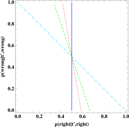
Figure 5: Allowed values for $(p(right|t^{\prime},right),p(wrong|t^{\prime},wrong))$ for $p(right|t,{\vec{x}_{s,a}})=1/2$ (dot dashed light blue line), $3/4$ (dashed green line), $1/2+1/(2\sqrt{2})$ (dotted red line) and $1$ (solid blue line).

As previously observed, the “amount” of uncertainty $\zeta_{\vec{x}_{s,a}}$ directly determines the violation of the CHSH inequality. In the quantum setting we have for all ${\vec{x}_{s,a}}$ that $\zeta_{\vec{x}_{s,a}}=1/2+1/(2\sqrt{2})\approx 0.853$, where for the individual probabilities we have for all $s$, $a$, $t$ and $b$

$$p(right|t,{\vec{x}_{s,a}})=\frac{1}{2}+\frac{1}{2\sqrt{2}}\ .$$ (76)

We also have that $p(right|t^{\prime},right)=p(right|t^{\prime},wrong)=1/2$ for all $t^{\prime}\neq t$. That is Bob’s optimal measurements are maximally complementary: Once Bob performed the first measurement, he can do no better than to guess the second bit. Note, however, that neither Eq. 75 nor letting $\zeta_{\vec{x}_{s,a}}=1/2+1/(2\sqrt{2})$ demands that quantum mechanics be maximally complementary without referring to the Hilbert space formalism. In particular, consider the average probability that Bob retrieves the $t^{\prime}$-th bit correctly after the measurement $t$ has already been performed which is given by

$$p_{\rm second} =p(right|t,{\vec{x}_{s,a}})p(right|t^{\prime},right)+ p(wrong|t,{\vec{x}_{s,a}})p(right|t^{\prime},wrong)\ .$$ (77)

We can use Eq. 75 to determine $p(right|t^{\prime},wrong)=1-p(wrong|t^{\prime},wrong)$. Using Eq. 76 we can now maximize $p_{\rm second}$ over the only free remaining variable $p(right|t^{\prime},right)$ such that $0\leq p(wrong|t^{\prime},wrong)\leq 1$. This gives us $p_{\rm second}=1-1/(2\sqrt{2})\approx 0.65$ which is attained for $p(right|t^{\prime},right)=2-\sqrt{2}\approx 0.59$ and $p(right|t^{\prime},wrong)=1$. However, for the measurements used by Bob’s optimal quantum strategy we only have $p_{\rm second}=1/2$. We thus see that it may be possible to have a physical theory which is as non-local and uncertain as quantum mechanics, but at the same time less complementary. We would like to emphasize, however, that in quantum theory it is known [25] that Bob’s observables must be maximally complementary in order to achieve Tsirelson’s bound, which is a consequence of the Hilbert space formalism.

Another interesting example is the case of a PR-boxes and other less non-local boxes. Here, we can have $p(right|t,{\vec{x}_{s,a}})=1-\varepsilon$ for all $t$, ${\vec{x}_{s,a}}$ and $1/2\leq\varepsilon\leq 1$. Note that for $\varepsilon\rightarrow 1$, maximising Eq. 77 gives us $p_{\rm second}=1/2$ with $p(right|t^{\prime},right)=1/2$. Figure 6 shows the value of $p_{\rm second}$ in terms of $p(right|t,{\vec{x}_{s,a}})$. If there is no uncertainty, we thus have maximal complementarity. However, as we saw from the example of quantum mechanics, for intermediate values of uncertainty, the degree of complementarity is not uniquely determined.

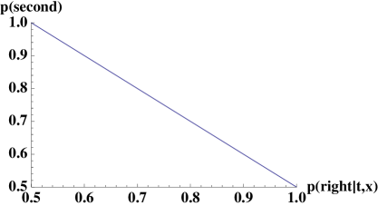
Figure 6: Maximum value of $p_{\rm second}$ subject to Eq. 75 in terms of $p(right|t,{\vec{x}_{s,a}})$.

It would be interesting to examine the role of comlementarity and its relation to non-locality in more detail. The existance of general monogamy relations [34] for example could be understood as a special form of complementarity when particular measurements are applied.

Appendix E From uncertainty relations to non-local games

In the body of the paper, we showed how every game corresponds to an uncertainty relation. Here we show that every uncertainty relation gives rise to a game. To construct the game from an uncertainty relation, we can simply go the other way.

We start with the set of inequalities

$$\mathcal{U}=\left\{\sum_{t=1}^{n}p(t)\ p(b_{t}|t)_{\sigma}\ \leq\zeta_{\vec{x}}\mid\forall{\vec{x}}\in\mathcal{B}^{\times n}\right\}\$$

which form the uncertainty relation. Additionally, they can be thought of as the average success probability that Bob will be able to correctly output the $t$’th entry from a string ${\vec{x}}$ .

Here, he is performing a measurement on the state $\sigma$ which encodes the string ${\vec{x}}$. The maximisation of these relations

$$P^{\rm succ}_{\Sigma}({\vec{x}})=\zeta_{\vec{x}}=\max_{\sigma\in\Sigma}\sum_{t=1}^{n}p(t)p(b_{t}|t)_{\sigma}\ ,$$ (78)

will play a key role, where here, the maximisation is taken over a set $\Sigma$ determined by the theory’s steering properties.

Consider the set of all strings ${\vec{x}}$ induced by the above uncertainty relation. We construct the game by choosing some partitioning of these strings into sets $P_{1},\ldots,P_{M}$ such that $\cup P_{s}=\mathcal{B}^{\times L}$. We we will challenge Alice to output one of the strings in set $s$ and Bob to output a certain entry $t$ of that string. Alice’s settings are given by $\mathcal{S}=\{1,\ldots,M\}$, that is, each setting will correspond to a set $P_{s}$. The outcomes for a setting $s\in\mathcal{S}$ are simply the strings contained in $P_{s}$, which using the notation from the main paper we will label ${\vec{x}_{s,a}}$.

Bob’s settings in the game are in one-to-one correspondence to the measurements for which we have an uncertainty relation. That is, we label his settings by his choices of measurements $\mathcal{T}=\{1,\ldots,n\}$ and his outcomes by the alphabet of the string. We furthermore, let the distributions over measurements be given by $p(t)$ as in the case of the uncertainty relation. Note that the distribution $p(s)$ over Alice’s measurement settings is not yet defined and may be chosen arbitrarily. The predicate is now simply defined as $V(a,b|s,t)=1$ if and only if $b_{t}$ is the $t$’th entry in the string ${\vec{x}_{s,a}}$.

Note that due to our construction, Alice will be able to steer Bob’s part of the state into some state $\sigma_{{\vec{x}_{s,a}}}$ encoding the string ${\vec{x}}$ for all settings $s$. We are then interested in the set of ensembles $\mathcal{I}=\{\mathcal{E}_{s}\}_{s}$ that the theory allows Alice to steer to. In no-signalling theories, this corresponds to probability distributions $\{p({\vec{x}}|s)\}_{s}$ and an average state $\rho$ such that

$$\sum_{{\vec{x}}\in P_{s}}p({\vec{x}}|s)\ \sigma_{\vec{x}}=\rho$$

As before, the states we can steer to in a particular ensemble $s$, we denote by $\Sigma_{s}$.

Now that we have defined the game this way, we obtain the following lower bound on the value $\omega(G)$ of the game.

$$\sum_{s}\sum_{a}p(s)p({{\vec{x}_{s,a}}}|s)P^{\rm succ}_{\Sigma_{s}}({\vec{x}_{s,a}})\leq{P^{\rm game}_{\rm max}}\ .$$ (79)

Whereas the measurements of our uncertainty relation do form a possible strategy for Alice and Bob, which due to the steering property can indeed be implemented, they may not be optimal. Indeed, there may exist an altogether different strategy consisting of different measurements and a different state in possibly much larger dimension that enables them to do significantly better.

However, having defined the game, we may now again consider a new uncertainty relation in terms of the optimal states and measurements for this game. For these optimal measurements, a violation of the uncertainty relations then lead to a violation of the corresponding Tsirelson’s bound and vice versa.

References

- [1] J. Allcock, N. Brunner, M. Pawlowski, and V. Scarani. Recovering part of the quantum boundary from information causality. http://arxiv.org/abs/0906.3464, 2009.
- [2] A. Ambainis, A. Nayak, A. Ta-Shma, and U. Vazirani. Quantum dense coding and a lower bound for 1-way quantum finite automata. In Proceedings of 31st ACM STOC, pages 376–383, 1999. http://arxiv.org/abs/quant-ph/9804043.
- [3] H. Barnum, S. Beigi, S. Boixo, M. Elliot, and S. Wehner. Local quantum measurement and no-signaling imply quantum correlations. Phys. Rev. Lett., 104:140401, 2010.
- [4] H. Barnum, C.P. Gaebler, and A. Wilce. Ensemble Steering, Weak Self-Duality, and the Structure of Probabilistic Theories. Imprint, 2009.
- [5] J. Barrett. Information processing in generalized probabilistic theories. Phys. Rev. A, 3:032304, 2007.
- [6] J. S. Bell. On the Einstein-Podolsky-Rosen paradox. Physics, 1:195–200, 1965.
- [7] I. Bialynicki-Birula and J. Mycielski. Uncertainty relations for information entropy in wave mechanics. Communications in Mathematical Physics, 44:129–132, 1975.
- [8] N. Bohr. Can quantum-mechanical description of physical reality be considered complete? Phys. Rev., 48(8):696–702, Oct 1935.
- [9] G. Brassard, H. Buhrman, N. Linden, A. Méthot, A. Tapp, and F. Unger. Limit on nonlocality in any world in which communication complexity is not trivial. Phys. Rev. Lett., 96(25):250401, 2006.
- [10] H. Buhrman and S. Massar. Causality and Cirel’son bounds. http://arxiv.org/abs/quant-ph/0409066, 2004.
- [11] J.F. Clauser, M.A. Horne, A. Shimony, and R.A. Holt. Proposed experiment to test local hidden-variable theories. Physical Review Letters, 23(15):880–884, 1969.
- [12] D. Deutsch. Uncertainty in quantum measurements. Phys. Rev. Lett., 50:631–633, 1983.
- [13] K. Dietz. Generalized bloch spheres for m-qubit states. Journal of Physics A: Math. Gen., 36(6):1433–1447, 2006.
- [14] A. C. Doherty, Y. Liang, B. Toner, and S. Wehner. The quantum moment problem and bounds on entangled multi-prover games. In Proceedings of IEEE Conference on Computational Complexity, pages 199–210, 2008.
- [15] D. Gopal and S. Wehner. On the use of post-measurement information in state discrimination. http://arxiv.org/abs/1003.0716, 2010.
- [16] W. Heisenberg. Über den anschaulichen Inhalt der quantentheoretischen Kinematik und Mechanik. Zeitschrift für Physik, 43:172–198, 1927.
- [17] S. Ji, J. Lee, J. Lim, K. Nagata, and H. Lee. Multisetting bell inequality for qudits. Phys. Rev. A, 78:052103, 2008.
- [18] S. J. Jones, H. M. Wiseman, and A.C.Doherty. Entanglement, epr-correlations, bell-nonlocality, and steering. Phys. Rev. A, 76:052116, 2007.
- [19] P. Jordan and E. Wigner. Über das paulische äquivalenzverbot. Zeitschrift für Physik, 47:631, 1928.
- [20] Y. Liang, C. Lim, and D. Deng. Reexamination of a multisetting bell inequality for qudits. Phys. Rev. A, 80:052116, 2009.
- [21] M. Navascués, S. Pironio, and A. Acin. Bounding the set of quantum correlations. Phys. Rev. Lett., 98:010401, 2007.
- [22] M. Navascués, S. Pironio, and A. Acin. A convergent hierarchy of semidefinite programs characterizing the set of quantum correlations. http://arxiv.org/abs/0803.4290, 2008.
- [23] A. Nayak. Optimal lower bounds for quantum automata and random access codes. In Proceedings of 40th IEEE FOCS, pages 369–376, 1999. http://arxiv.org/abs/quant-ph/9904093.
- [24] M. Pawlowski, T. Paterek, D. Kaszlikowski, V. Scarani, A. Winter, and M. Zukowski. Information causality as a physical principle. Nature, 461(7267):1101–1104, 2009.
- [25] A. Peres. Quantum Theory: Concepts and Methods. Kluwer Academic Publishers, 1993.
- [26] S. Popescu and D. Rohrlich. Quantum nonlocality as an axiom. Foundations of Physics, 24(3):379–385, 1994.
- [27] S. Popescu and D. Rohrlich. Nonlocality as an axiom for quantum theory. In A. Mann and M. Revzen, editors, The dilemma of Einstein, Podolsky and Rosen, 60 years later: International symposium in honour of Nathan Rosen. Israel Physical Society, Haifa, Israel, 1996. http://arxiv.org/abs/quant-ph/9508009.
- [28] S. Popescu and D. Rohrlich. Causality and nonlocality as axioms for quantum mechanics. In Geoffrey Hunter, Stanley Jeffers, and Jean-Pierre Vigier, editors, Proceedings of the Symposium of Causality and Locality in Modern Physics and Astronomy: Open Questions and Possible Solutions, page 383. Kluwer Academic Publishers, Dordrecht/Boston/London, 1997. http://arxiv.org/abs/quant-ph/9709026.
- [29] P. Rastall. Locality, Bell’s theorem and quantum mechanics. Foundations of Physics, 15(9), 1985.
- [30] E. Schrödinger. Discussion of probability relations between separated systems. Proc. Cambridge Phil. Soc., 31:553, 1935.
- [31] E. Schrödinger. Probability relations between separated systems. Proc. Cambridge Phil. Soc., 32:446, 1936.
- [32] R.W. Spekkens. In defense of the epistemic view of quantum states: a toy theory. http://arxiv.org/abs/quant-ph/0401052, 2004.
- [33] G. Ver Steeg and S. Wehner. Relaxed uncertainty relations and information processing. QIC, 9(9):801, 2009.
- [34] B. Toner and F. Verstraete. Monogamy of Bell correlations and Tsirelson’s bound. http://arxiv.org/abs/quant-ph/0611001, 2006.
- [35] B. Tsirelson. Quantum generalizations of Bell’s inequality. Letters in Mathematical Physics, 4:93–100, 1980.
- [36] B. Tsirelson. Quantum analogues of Bell inequalities: The case of two spatially separated domains. Journal of Soviet Mathematics, 36:557–570, 1987.
- [37] BS Tsirelson. Some results and problems on quantum Bell-type inequalities. Hadronic Journal Supplement, 8(4):329–345, 1993. http://www.tau.ac.il/~tsirel/download/hadron.html.
- [38] W. van Dam. Impossible consequences of superstrong nonlocality. quant-ph/0501159, 2005.
- [39] S. Wehner. Tsirelson bounds for generalized Clauser-Horne-Shimony-Holt inequalities. Physical Review A, 73:022110, 2006. http:/arxiv.org/abs/quant-ph/0510076.
- [40] S. Wehner, M. Christandl, and A. C. Doherty. A lower bound on the dimension of a quantum system given measured data. Phys. Rev. A, 78:062112, 2008.
- [41] S. Wehner and A. Winter. Higher entropic uncertainty relations for anti-commuting observables. Journal of Mathematical Physics, 49:062105, 2008.
- [42] S. Wehner and A. Winter. Entropic uncertainty relations – A survey. New Journal of Physics, 12:025009, 2010. Special Issue on Quantum Information and Many-Body Theory.
- [43] H.M. Wiseman, S.J. Jones, and A.C. Doherty. Steering, entanglement, nonlocality, and the epr paradox. Phys. Rev. Lett., 98:140402, 2007.
- [44] M.M. Wolf, D. Perez-Garcia, and C. Fernandez. Measurements incompatible in quantum theory cannot be measured jointly in any other local theory. Phys. Rev. Lett., 103:230402, 2009.
- [45] W. K. Wootters and D. M. Sussman. Discrete phase space and minimum-uncertainty states. http://arxiv.org/abs/0704.1277, 2007.