Derivation of a Stochastic Neutron Transport Equation

Abstract

Stochastic difference equations and a stochastic partial differential equation (SPDE) are simultaneously derived for the time-dependent neutron angular density in a general three-dimensional medium where the neutron angular density is a function of position, direction, energy, and time. Special cases of the equations are given such as transport in one-dimensional plane geometry with isotropic scattering and transport in a homogeneous medium. The stochastic equations are derived from basic principles, i.e., from the changes that occur in a small time interval. Stochastic difference equations of the neutron angular density are constructed, taking into account the inherent randomness in scatters, absorptions, and source neutrons. As the time interval decreases, the stochastic difference equations lead to a system of Itô stochastic differential equations (SDEs). As the energy, direction, and position intervals decrease, an SPDE is derived for the neutron angular density. Comparisons between numerical solutions of the stochastic difference equations and independently formulated Monte Carlo calculations support the accuracy of the derivations.

This paper is to be published in the Journal of Difference Equations and Applications.

Short running title: Stochastic Neutron Transport

Keywords: stochastic partial differential equation; neutron transport equation; Itô system; stochastic model; Boltzmann transport equation.

Mathematics subject classification: AMS(MOS) 82D75, 60H15, 82C70, 60H10, 65C30.

1 Introduction

In the present investigation, stochastic versions of the deterministic neutron transport equation are derived. Specifically, stochastic difference equations and a stochastic partial differential equation (SPDE) are simultaneously derived that account for the random effects of absorptions, scatters, and source particles and generalize the standard deterministic neutron transport equation. Numerical approximations of the SPDE, through solution of the system of stochastic difference equations, provide approximations to the randomly varying neutron densities and yield insight into the random behavior of neutron transport. The stochastic transport equations are most useful for problems involving low numbers of neutrons. As the coefficient of variation is often approximately inversely proportional to the square root of the population size, the deterministic and stochastic transport equations yield essentially the same results for high numbers of neutrons.

There are alternate but apparently equivalent ways to derive a system of stochastic differential equations (SDEs) for a randomly varying dynamical problem. The first way involves deriving a master equation for the random process [14, 26]. A master equation is a differential form of the Chapman-Kolmogorov equation involving transition probabilities and is a probability conservation equation for the probabilities of separate states. If the transition densities are expanded in a parameter that defines the size of the fluctuations or jumps, then a Fokker-Planck equation or forward Kolmogorov equation is obtained in the first few terms of the expansion. As the probability density of an SDE system satisfies a certain forward Kolmogorov equation, this procedure infers a particular SDE system that approximates the random dynamics of the problem. In this procedure, a system of stochastic difference equations is not derived as an intermediate step. A second way to derive a system of SDEs for a randomly varying problem is by studying the changes in the process for a short time interval which gives a discrete stochastic model. The discrete stochastic model infers a system of stochastic difference equations which, in turn, leads to an appropriate SDE system. For example, consider a randomly varying problem where $\vec{X}=[X_{1},X_{2},\dots,X_{N}]^{T}$ is a random vector of $N$ components for the problem. Let $\Delta\vec{X}$ be the change in the process for a small time interval $\Delta t$. The expectations $\vec{\mu}(\vec{X},t)=E(\Delta\vec{X})/\Delta t$ and $V(\vec{X},t)=E(\Delta\vec{X}(\Delta\vec{X})^{T})/\Delta t$ are determined and a stochastic difference equation approximation for the problem has the form:

$$\vec{X}(t+\Delta t)=\vec{X}(t)+\vec{\mu}(\vec{X}(t),t)\Delta t+(V(\vec{X}(t),t))^{1/2}\;\sqrt{\Delta t}\;\vec{\eta}_{t}$$ (1)

where $\vec{\eta}_{t}$ is a vector of length $N$ of independent normally distributed random numbers with zero mean and unit variance. Finally, the SDE system that approximates the behavior of the randomly varying process has the form

$$d\vec{X}(t)=\vec{\mu}(\vec{X},t)dt+(V(\vec{X},t))^{1/2}\;d\vec{W}(t)$$ (2)

where $\vec{W}(t)$ is a vector of length $N$ of independent Wiener processes. It can be shown that the probability density of solutions of the stochastic system (1) or (2) approximates the probability density of the original randomly varying process [1, 4, 6]. Assume now that there are $M$ possible changes in the process with probabilities $p_{j}\Delta t$ for $j=1,2,\dots,M$ for small $\Delta t$. Also, assume that the $j$th change alters the $i$th component by $\lambda_{j,i}$. Then, the elements of $\vec{\mu}$ are given by $\mu_{i}=\sum_{j=1}^{M}p_{j}\lambda_{j,i}$ and the elements of $N\times N$ matrix $V$ are given by $v_{i,l}=\sum_{j=1}^{M}p_{j}\lambda_{j,i}\lambda_{j,l}$ for $i,l=1,2,\dots N$. In addition, an equivalent SDE system to (2) is

$$d\vec{X}(t)=\vec{\mu}(\vec{X},t)dt+C(\vec{X},t)\;d\vec{W}^{*}(t)$$ (3)

where $N\times M$ matrix $C$ has elements $c_{i,j}=\lambda_{j,i}p_{j}^{1/2}$ and $\vec{W}^{*}(t)$ is a vector of length $M$ of independent Wiener processes. Furthermore, equation (3) is also obtained from the master-equation approach under the same assumptions [14]. Thus, the two derivation procedures produce identical SDE systems for this general $N$-component and $M$-change process.

These two derivation procedures produce very reasonable stochastic equation models for a given phenomenon. For randomly varying systems where the dependent variable depends on time and on secondary independent variables, a stochastic partial differential equation (SPDE) may be derived by replacing the Wiener processes in the SDE system with appropriate Brownian sheets and letting the intervals in the remaining independent variables go to zero. The resulting equation is an SPDE model for the phenomenon.

In this paper, stochastic difference equations and a stochastic partial differential equation are derived for the transport of neutrons in matter. In neutron transport, captures, scatters, fissions, and source neutrons occur randomly. As a result, the neutron angular density varies stochastically. The relative magnitude of the random behavior of the angular density is pronounced for low neutron densities, such as during reactor startup, but decreases as the neutron density increases. The standard or deterministic neutron transport equation (or Boltzmann neutron transport equation) describes the expected or probable neutron angular density with respect to position, direction, energy, and time [9]. Solutions of the deterministic neutron transport equation provide average values of the neutron angular density; actual realizations with time of the neutron angular densities, that include random effects from neutron interactions and sources, are not obtained.

A stochastic partial differential equation is derived in this paper for neutron transport in a general three-dimensional absorbing and anisotropic-scattering medium where the neutron angular density depends on position, direction, energy, and time. In the present investigation, the medium is assumed to be constant with respect to material composition, i.e., zero power noise. Special random effects, for example, from randomly varying boundary conditions or from a medium that is randomly varying [28, 29] are not studied in the present investigation although generalizations of the SPDE to approximate such conditions may be possible. Using the derived stochastic neutron transport equation, sample paths (realizations) of the randomly varying neutron angular densities can be approximately computed. In addition, after computing many sample paths, moments of the neutron densities, for example, can be estimated. The stochastic neutron transport equation is derived from basic principles, i.e., from the changes in the system that occur in a small time interval. The dynamical system is studied to determine the different independent random changes that occur. Appropriate terms are identified for these changes in developing a stochastic difference system where all independent variables are discrete. As the time interval goes to zero, a certain stochastic differential equation (SDE) system is inferred (e.g., [1, 4, 6, 16, 25]). Next, multidimensional Brownian sheets replace the Wiener processes. As the intervals in the remaining independent variables go to zero, the SDE system leads to an SPDE [2, 3]. It is illustrated how the stochastic transport equation can be solved computationally through numerical solution of a stochastic difference system.

The neutron transport equation is of fundamental importance in nuclear reactor theory and shielding design [9, 12, 17, 22]. The stochastic nature of the neutron transport process has been of interest for many years. Classic studies of the stochastic theory of neutron transport are given in [7, 8]. In particular, let $p_{n}(R,t_{f};\vec{x},\vec{v},t)$ be the probability that a neutron with position $\vec{x}$ and velocity $\vec{v}$ at time $t$ leads to $n$ neutrons in region $R$ of $\vec{x},\vec{v}$ space at time $t_{f}$. In [8], a non-linear integro-differential equation for the probability generating function is derived for $p_{n}(R,t_{f};\vec{x},\vec{v},t)$. The equations derived are interesting but complicated and difficult to apply. More recently, a master equation approach was used to estimate the temporal evolution of the number of neutrons in time-varying multiplying systems [19, 23]. This approach gives, for example, moments of the number of neutrons in the system with time. However, a stochastic difference system approximation of neutron transport is not determined and, as a result, sample paths of the randomly varying neutron densities with respect to energy, position, and direction are not estimated.

In the next section, stochastic difference equations and a stochastic partial differential equation are derived for neutron transport in general three-dimensional xyz-geometry. The changes due to absorptions, fissions, and scatters, which occur randomly with probability proportional to the neutron angular density and to the time interval, are carefully considered in deriving the equations. In the third section, several special but useful cases of the stochastic neutron transport equation are described such as one-dimensional slab geometry with isotropic scattering. In the fourth section, stochastic difference equations are solved computationally for the randomly varying neutron densities and compared with Monte Carlo calculations. The Monte Carlo calculational procedures differ considerably from the numerical solution of the stochastic transport equations. In the Monte Carlo calculations, the dynamical system is checked at each small interval of time to take into account scatters, absorptions, and movements for individual neutrons. Comparisons between the two different computational methods are in close agreement indicating that the stochastic difference equations and the stochastic partial differential equation accurately model the random behavior of neutron transport. Although the stochastic equations cannot exactly model the random behavior of neutron transport since, for example, the number of neutrons in any region is not integer-valued in the stochastic difference system or in the SPDE model, the calculations indicate that the stochastic neutron transport model is accurate. In addition, the stochastic transport equations provide insight into the random dynamics of neutron transport and can be efficiently solved computationally using the stochastic difference equations. Several applications of the stochastic neutron transport equation are discussed in the fifth section before the investigation is summarized in the final section.

2 Derivation of Stochastic Neutron Transport Equations

The neutron transport equation in xyz-geometry can be written in the integro-differential form [9, 12]:

$$\dfrac{\partial\bar{N}(x,y,z,\mu,\phi,E,t)}{\partial t}=-v\mu_{x}\dfrac{\partial\bar{N}}{\partial x}-v\mu_{y}\dfrac{\partial\bar{N}}{\partial y}-v\mu_{z}\dfrac{\partial\bar{N}}{\partial z}$$ (4)

$$+\,Q(x,y,z,E,t)-v\sigma(x,y,z,E)\bar{N}(x,y,z,\mu,\phi,E)$$

$$+\int_{0}^{E_{max}}\int_{-1}^{1}\int_{0}^{2\pi}v^{\prime}\sigma^{\prime}f(x,y,z,\mu^{\prime},\phi^{\prime},E^{\prime},\mu,\phi,E)\bar{N}^{\prime}\;d\phi^{\prime}d\mu^{\prime}dE^{\prime}$$

for $(x,y,z)\in([0,x_{max}]\times[0,y_{max}]\times[0,z_{max}])\subset\mathbb{R}^{3}$, $-1\leq\mu\leq 1$, $0\leq\phi\leq 2\pi$, $0\leq E\leq E_{max}$ and $t\geq 0$ where $\bar{N}=\bar{N}(x,y,z,\mu,\phi,E,t)$ is the expected neutron angular density with respect to position $(x,y,z)$, direction $\vec{\Omega}=(\mu,\phi)$, energy $E$, and time $t$ per unit volume per unit solid angle per unit energy. In (4), $\sigma^{\prime}=\sigma(x,y,z,E^{\prime})$ and $\bar{N}^{\prime}=\bar{N}(x,y,z,\mu^{\prime},\phi^{\prime},E^{\prime},t)$. The notation used here is generally consistent with the notation used in [9]. In particular, $v$ is the neutron speed, $\sigma$ is the total macroscopic cross section, $\sigma(x,y,z,E^{\prime})f(x,y,z,\mu^{\prime},\phi^{\prime},E^{\prime},\mu,\phi,E)\Delta\mu\Delta\phi\Delta E$ is the probability of a neutron transfer from direction $(\mu^{\prime},\phi^{\prime})$ and energy $E^{\prime}$ to solid angle $\Delta\mu\Delta\phi$ about direction $(\mu,\phi)$ with energy $\Delta E$ about energy $E$. Note that

$$\sigma^{\prime}f(x,y,z,\mu^{\prime},\phi^{\prime},E^{\prime},\mu,\phi,E)=\sum_{r}\sigma_{r}^{\prime}f_{r}(x,y,z,\mu^{\prime},\phi^{\prime},E^{\prime},\mu,\phi,E)$$

where $\sigma_{r}^{\prime}=\sigma_{r}(x,y,z,E^{\prime})$ and the sum includes the separate interactions $r$ in which neutrons are produced such as elastic scattering or fission. The parameters $\mu_{x}$, $\mu_{y}$ and $\mu_{z}$ are the direction cosines for the $x$, $y$, and $z$ axes, respectively. In particular, $\mu_{x}=\mu=\cos\theta$, $\mu_{y}=\sin(\cos^{-1}\mu)\cos\phi$, and $\mu_{z}=\sin(\cos^{-1}\mu)\sin\phi$. Thus, $\vec{\Omega}\cdot\vec{\nabla}\bar{N}=\mu_{x}\dfrac{\partial\bar{N}}{\partial x}+\mu_{y}\dfrac{\partial\bar{N}}{\partial y}+\mu_{z}\dfrac{\partial\bar{N}}{\partial z}$. Furthermore, $c(x,y,z,E)=\int_{0}^{E_{max}}\int_{-1}^{1}\int_{0}^{2\pi}f(x,y,z,\mu,\phi,E,\mu^{\prime},\phi^{\prime},E^{\prime})\;d\phi^{\prime}d\mu^{\prime}dE^{\prime}$ is the mean number of neutrons emerging per collision of neutrons of energy $E$ at position $(x,y,z)$. Finally, $Q(x,y,z,E)$ is the number of source neutrons per unit solid angle per unit volume per unit energy and is assumed to be isotropic.

To simplify the derivation, it is useful to define several other quantities. Let $\sigma_{c}$ be the capture cross section, i.e., the sum of all the cross sections involving a pure capture event such as those due to $(n,\gamma),(n,p)$, or $(n,\alpha)$ collisions. Let $\hat{\sigma}(x,y,z,E)=\sigma(x,y,z,E)-\sigma_{c}(x,y,z,E)$ be the macroscopic cross section for all interactions other than pure capture interactions. Let $\hat{f}$ be defined by the expression

$$\hat{\sigma}(x,y,z,E^{\prime})\hat{f}(x,y,z,\mu^{\prime},\phi^{\prime},E^{\prime},\mu,\phi,E)=\sigma^{\prime}f(x,y,z,\mu^{\prime},\phi^{\prime},E^{\prime},\mu,\phi,E)$$

and define $\hat{c}(x,y,z,E)=\int_{0}^{E_{max}}\int_{-1}^{1}\int_{0}^{2\pi}\hat{f}(x,y,z,\mu,\phi,E,\mu^{\prime},\phi^{\prime},E^{\prime})\;d\phi^{\prime}d\mu^{\prime}dE^{\prime}$ as the mean number of neutrons emerging per non-capture collision of neutrons of energy $E$ at position $(x,y,z)$.

Equation (4) is deterministic and random variations in the neutron angular density due to the inherent randomness in absorptions, scatters, and fissions cannot be accurately studied using this equation. To derive a stochastic partial differential equation generalization of (4), the changes which occur in the angular density for a small time interval are determined taking into account interactions and transport. A discrete stochastic model of the neutron angular density is then constructed which infers a system of stochastic difference equations. As the time interval decreases, the stochastic difference system leads to a system of Itô stochastic differential equations. As the intervals in position, direction, and energy decrease, a stochastic partial differential equation is derived for the neutron transport process.

2.1 Several Properties of Brownian Sheets

Before deriving these stochastic equations, it is useful to consider several properties of Brownian sheets [5, 10, 27]. A Brownian sheet on $[0,5]\times[0,5]$ is illustrated in Fig. 1.

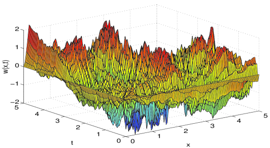
Figure 1: A Brownian sheet on $[0,5]\times[0,5]$.

The Brownian sheet $W(x,t)$ satisfies:

$$\int_{t}^{t+\Delta t}\int_{x}^{x+\Delta x}\dfrac{\partial^{2}W(x^{\prime},t^{\prime})}{\partial t^{\prime}\partial x^{\prime}}\,dx^{\prime}\,dt^{\prime}\sim{\mathcal{N}}(0,\Delta x\Delta t).$$

That is, the Brownian sheet is independent and normally distributed over rectangular regions. In addition, if $x_{j}=j\Delta x$ for $j=0,1,\dots,J$, where $\Delta x=x_{max}/J$, then the Brownian sheet defines for $j=1,2,\dots J$, the standard Wiener processes, $W_{j}(t)$, where

$$\dfrac{dW_{j}(t)}{dt}=\dfrac{1}{\sqrt{\Delta x}}\int_{x_{j-1}}^{x_{j}}\dfrac{\partial^{2}W(x^{\prime},t)}{\partial t\partial x^{\prime}}\,dx^{\prime}.$$

Notice that if $t_{i}=i\Delta t$ for $i=0,1,\dots,M$, then

$$\int_{t_{i-1}}^{t_{i}}dW_{j}(t^{\prime})=\sqrt{\Delta t}\,\eta_{i,j}$$

where $\eta_{i,j}\sim{\mathcal{N}}(0,1)$ for each $j=1,2,\dots J$ and $i=1,2,\dots M$. Also, standard Wiener processes can be defined using, for example, three-dimensional Brownian sheets letting

$$dW_{j,k}(t)=\dfrac{1}{\sqrt{\Delta x\Delta y}}\int_{x_{j-1}}^{x_{j}}\int_{y_{k-1}}^{y_{k}}\dfrac{\partial^{3}W(x^{\prime},y^{\prime},t)}{\partial t\partial y^{\prime}\partial x^{\prime}}\,dy^{\prime}dx^{\prime}dt$$

where $W_{j,k}(t)$ is a Wiener process for each $j$ and $k$. However, notice that

$$\dfrac{\partial^{3}W(x,y,t)}{\partial t\partial y\partial x}=\lim_{\Delta x,\Delta y\to 0}\dfrac{1}{\Delta x\Delta y}\int_{x}^{x+\Delta x}\int_{y}^{y+\Delta y}\dfrac{\partial^{3}W(x^{\prime},y^{\prime},t)}{\partial t\partial y^{\prime}\partial x^{\prime}}\,dy^{\prime}dx^{\prime}.$$

Finally, it is useful to note that $W(x,t)\neq W_{1}(x)W_{2}(t)$ where $W_{1}(x)$ and $W_{2}(t)$ are independent Wiener processes. To see this, let $A=[a,b]\times[c,d]$ and $|A|=(d-c)(b-a)$. Then,

$${\displaystyle W(A)=\int_{a}^{b}\int_{c}^{d}\dfrac{\partial^{2}W(x,t)}{\partial t\partial x}\;dxdy=W(b,d)-W(b,c)-W(a,d)+W(a,c)\sim\mathcal{N}(0,|A|).}$$

In particular, $W(A)=\sqrt{|A|}\;\eta_{xt}$ where $\eta_{xt}\sim\mathcal{N}(0,1)$. However,

$$W_{1,2}(A)=\int_{a}^{b}\int_{c}^{d}dW_{1}(x)dW_{2}(t)=(W_{1}(b)-W_{1}(a))(W_{2}(d)-W_{2}(c))=\sqrt{|A|}\;\eta_{x}\eta_{t}$$

where $\eta_{x}\sim\mathcal{N}(0,1)$ and $\eta_{t}\sim\mathcal{N}(0,1)$. So, for example, $E((W(A))^{4})=3|A|^{2}$ whereas $E((W_{1,2}(A))^{4})=9|A|^{2}$.

2.2 Derivation of stochastic neutron transport equations

To derive a stochastic neutron transport equation, the changes which occur in the neutron angular density for a small time interval $\Delta t$ at time $t_{p}$ are considered where $t_{p}=(p-1)\Delta t$ for $p=1,2,\dots.$ To facilitate finding these changes, the variables position, direction, and energy are made discrete. Three-dimensional space is discretized into rectangular parallelepipeds of length, width, and height $\Delta x,\Delta y,\Delta z$, respectively. The direction variables $\mu$ and $\phi$ are discretized with intervals of size $\Delta\mu=2/L$ and $\Delta\phi=2\pi/M$, and energy is discretized into intervals of size $\Delta E=E_{max}/G$. Furthermore, $x_{i}=(i-1)\Delta x$ for $i=1,2,\dots,I+1$, $y_{j}=(j-1)\Delta y$ for $j=1,2,\dots,J+1$, $z_{k}=(k-1)\Delta z$ for $k=1,2,\dots,K+1$, $\mu_{l}=-1+(l-1)\Delta\mu$ for $l=1,2,\dots,L+1$, $\phi_{m}=(m-1)\Delta\phi$ for $m=1,2,\dots,M+1$, and $E_{g}=(g-1)\Delta E$ for $g=1,2,\dots,G+1$. Now let $n(x_{i},y_{j},z_{k},\mu_{l},\phi_{m},E_{g},t_{p})=N(x_{i},y_{j},z_{k},\mu_{l},\phi_{m},E_{g},t_{p})\Delta x\Delta y\Delta z\Delta\mu\Delta\phi\Delta E$ be the number of neutrons in the parallelepiped moving in direction $\mu_{l},\phi_{m}$ with energy $E_{g}$. There are several possible changes that can occur to $n=n(x_{i},y_{j},z_{k},\mu_{l},\phi_{m},E_{g},t_{p})$ in the small time interval $\Delta t$. A capture or fission can occur, a neutron can enter or leave one of the six faces of the parallelepiped, or a scatter can occur resulting in a loss or gain of one neutron. The possible changes $\Delta n$ along with their probabilities are listed in Table 1 for a small time interval $\Delta t$. Notice that position changes occur deterministically, i.e., the neutron position is determined by the neutron velocity and, thus, the number of neutrons moving from one parallelepiped into an adjacent parallelepiped is calculated based on the fraction of neutrons crossing the parallelepiped boundary in time $\Delta t$. In Table 1, the probabilities $p_{c},p_{tr1},p_{tr2}$, and $p_{Q}$ are given by

$$p_{c} = v_{g}\sigma_{c}n(x_{i},y_{j},z_{k},\mu_{l},\phi_{m},E_{g},t_{p})\Delta t$$

$$p_{tr1} = v_{g}\hat{\sigma}\hat{f}n\Delta\mu\Delta\phi\Delta E\Delta t,$$

$$p_{tr2} = v_{g^{\prime}}\sigma^{\prime}f^{\prime}n^{\prime}\Delta\mu\Delta\phi\Delta E\Delta t,\;\;\text{and}$$

$$p_{Q} = Q(x_{i},y_{j},z_{k},E_{g},t_{p})\Delta x\Delta y\Delta z\Delta\mu\Delta\phi\Delta E\Delta t.$$

For example, in Table 1, $v_{g}\sigma_{c}(x_{i},y_{j},z_{k},E_{g})n(x_{i},y_{j},z_{k},\mu_{l},\phi_{m},E_{g},t_{p})\Delta t$ is the probability that a neutron in the packet undergoes a capture. However, the two interaction terms, i.e., the term involving transfer into the packet and the term involving transfer out of the packet, need to be considered at each position for all the different directions and energies. Specifically,

$$p_{tr1}=v_{g}\hat{\sigma}\hat{f}(x_{i},y_{j},z_{k},\mu_{l},\phi_{m},E_{g},\mu_{l^{\prime}},\phi_{m^{\prime}},E_{g^{\prime}})n\Delta\mu\Delta\phi\Delta E\Delta t$$

is the probability in time $\Delta t$ that $1/\hat{c}(x_{i},y_{j},z_{k},E_{g})$ neutrons are lost from direction $\mu_{l},\phi_{m}$ at energy $E_{g}$ (from the packet) when one neutron emerges in direction $\mu_{l^{\prime}},\phi_{m^{\prime}}$ with energy $E_{g^{\prime}}$ for each value of $l^{\prime}$, $m^{\prime}$, and $g^{\prime}$ and

$$p_{tr2}=v_{g^{\prime}}\sigma^{\prime}f(x_{i},y_{j},z_{k},\mu_{l^{\prime}},\phi_{m^{\prime}},E_{g^{\prime}},\mu_{l},\phi_{m},E_{g})n^{\prime}\;\Delta\mu\Delta\phi\Delta E\Delta t$$

is the probability that one neutron emerges in direction $\mu_{l},\phi_{m}$ at energy $E_{g}$ (into the packet) when $1/\hat{c}(x_{i},y_{j},z_{k},E_{g^{\prime}})$ neutrons are lost from direction $\mu_{l^{\prime}},\phi_{m^{\prime}}$ and energy $E_{g^{\prime}}$ for each value of $l^{\prime}$, $m^{\prime}$, and $g^{\prime}$. Note, for convenience in Table 1, $n=n(x_{i},y_{j},z_{k},\mu_{l},\phi_{m},E_{g},t_{p})$, $n^{\prime}=n(x_{i},y_{j},z_{k},\mu_{l^{\prime}},\phi_{m^{\prime}},E_{g^{\prime}},t_{p})$, $\sigma=\sigma(x_{i},y_{j},z_{k},E_{g})$, $\sigma^{\prime}=\sigma(x_{i},y_{j},z_{k},E_{g^{\prime}})$, $\sigma_{c}=\sigma_{c}(x_{i},y_{j},z_{k},E_{g}),\;$ $\hat{\sigma}=\hat{\sigma}(x_{i},y_{j},z_{k},E_{g}),\;$ $\hat{f}=\hat{f}(x_{i},y_{j},z_{k},\mu_{l},\phi_{m},E_{g},\mu_{l^{\prime}},\phi_{m^{\prime}},E_{g^{\prime}})$, $f^{\prime}=f(x_{i},y_{j},z_{k},\mu_{l^{\prime}},\phi_{m^{\prime}},E_{g^{\prime}},\mu_{l},\phi_{m},E_{g})$, and $\hat{c}=\hat{c}(x_{i},y_{j},z_{k},E_{g})$. Also, it is assumed that the neutron source, $Q$, is a Poisson process with the probability of adding one source neutron to the packet in a small time interval $\Delta t$ equal to $Q(x_{i},y_{j},z_{k},E_{g},t_{p})\Delta x\Delta y\Delta z\Delta\mu\Delta\phi\Delta E\Delta t$.

Table 1 defines a discrete stochastic model for the neutron transport system. Using these changes and probabilities and letting the time interval $\Delta t$ approach zero, a system of Itô stochastic differential equations can be formulated for the dynamics of this random transport process. First, a deterministic equation for the expected number of neutrons at time $t_{p}+\Delta t$ can be derived using the results of the Table 1. This equation, for $\mu_{x},\mu_{y},\mu_{z}>0$, is given by:

$$\bar{n}(x_{i},y_{j},z_{k},\mu_{l},\phi_{m},E_{g},t_{p}+\Delta t)=\bar{n}(x_{i},y_{j},z_{k},\mu_{l},\phi_{m},E_{g},t_{p})$$ (5)

$$-v_{g}\sigma_{c}\bar{n}(x_{i},y_{j},z_{k},\mu_{l},\phi_{m},E_{g},t_{p})\Delta t$$

$$+\mu_{x}v_{g}\Delta t(\bar{n}(x_{i-1},y_{j},z_{k},\mu_{l},\phi_{m},E_{g},t_{p})-\bar{n}(x_{i},y_{j},z_{k},\mu_{l},\phi_{m},E_{g},t_{p}))/\Delta x$$

$$+\mu_{y}v_{g}\Delta t(\bar{n}(x_{i},y_{j-1},z_{k},\mu_{l},\phi_{m},E_{g},t_{p})-\bar{n}(x_{i},y_{j},z_{k},\mu_{l},\phi_{m},E_{g},t_{p}))/\Delta y$$

$$+\mu_{z}v_{g}\Delta t(\bar{n}(x_{i},y_{j},z_{k-1},\mu_{l},\phi_{m},E_{g},t_{p})-\bar{n}(x_{i},y_{j},z_{k},\mu_{l},\phi_{m},E_{g},t_{p}))/\Delta z$$

$$+Q(x_{i},y_{j},z_{k},E_{g},t_{p})\Delta x\Delta y\Delta z\Delta\mu\Delta\phi\Delta E\Delta t$$

$$-\sum_{l^{\prime}=1}^{L}\sum_{m^{\prime}=1}^{M}\sum_{g^{\prime}=1}^{G}\dfrac{1}{\hat{c}}v_{g}\hat{\sigma}\hat{f}(x_{i},y_{j},z_{k},\mu_{l},\phi_{m},E_{g},\mu_{l^{\prime}},\phi_{m^{\prime}},E_{g^{\prime}})\bar{n}\Delta\mu\Delta\phi\Delta E\Delta t$$

$$+\sum_{l^{\prime}=1}^{L}\sum_{m^{\prime}=1}^{M}\sum_{g^{\prime}=1}^{G}v_{g^{\prime}}\sigma^{\prime}f(x_{i},y_{j},z_{k},\mu_{l^{\prime}},\phi_{m^{\prime}},E_{g^{\prime}},\mu_{l},\phi_{m},E_{g})\bar{n}^{\prime}\Delta\mu\Delta\phi\Delta E\Delta t$$

where $\bar{n}$ is the expected number of neutrons in the packet. Letting $\bar{n}=\bar{N}\Delta x\Delta y\Delta z\Delta\mu\Delta\phi\Delta E$ and allowing $\Delta t$ to approach zero as well as $\Delta x$, $\Delta y$, $\Delta z$, $\Delta\mu$, $\Delta\phi,$ and $\Delta E$, it is straightforward to show that (5) yields the standard neutron transport equation (4). However, the changes and probabilities given in Table 1 can be used to derive an SDE model. Indeed, the discrete stochastic model and the SDE model will have approximately the same covariance terms as well as mean terms for small $\Delta t$.

The derivation procedure, described in the Introduction for obtaining equation (3), is now applied using the changes and probabilities given in Table 1 to obtain the stochastic terms in the equations. Specifically, for the $i$th component (packet) of the system, the coefficient of the independent Wiener process corresponding to the $j$th change is equal to the product of $\lambda_{j,i}$ with the square root of the probability for the $j$th change, recalling that $\lambda_{j,i}$ is the amount that the $j$th change alters the $i$th component. The changes and probabilities given in Table 1 imply, for $\mu_{x},\mu_{y},\mu_{z}>0$, that a very reasonable approximation to the discrete stochastic model satisfies the stochastic difference system:

$$n(x_{i},y_{j},z_{k},\mu_{l},\phi_{m},E_{g},t+\Delta t)=n(x_{i},y_{j},z_{k},\mu_{l},\phi_{m},E_{g},t)$$ (6)

$$+\mu_{x}v_{g}(n(x_{i-1},y_{j},z_{k},\mu_{l},\phi_{m},E_{g},t)-n(x_{i},y_{j},z_{k},\mu_{l},\phi_{m},E_{g},t))\Delta t/\Delta x$$

$$+\mu_{y}v_{g}(n(x_{i},y_{j-1},z_{k},\mu_{l},\phi_{m},E_{g},t)-n(x_{i},y_{j},z_{k},\mu_{l},\phi_{m},E_{g},t))\Delta t/\Delta y$$

$$+\mu_{z}v_{g}(n(x_{i},y_{j},z_{k-1},\mu_{l},\phi_{m},E_{g},t)-n(x_{i},y_{j},z_{k},\mu_{l},\phi_{m},E_{g},t))\Delta t/\Delta z$$

$$+Q(x_{i},y_{j},z_{k},E_{g},t)\Delta x\Delta y\Delta z\Delta\mu\Delta\phi\Delta E\Delta t-v_{g}\sigma_{c}n(x_{i},y_{j},z_{k},\mu_{l},\phi_{m},E_{g},t)\Delta t$$

$$-\sum_{l^{\prime}=1}^{L}\sum_{m^{\prime}=1}^{M}\sum_{g^{\prime}=1}^{G}\dfrac{1}{\hat{c}}v_{g}\hat{\sigma}\hat{f}(x_{i},y_{j},z_{k},\mu_{l},\phi_{m},E_{g},\mu_{l^{\prime}},\phi_{m^{\prime}},E_{g^{\prime}})n\Delta\mu\Delta\phi\Delta E\Delta t$$

$$+\sum_{l^{\prime}=1}^{L}\sum_{m^{\prime}=1}^{M}\sum_{g^{\prime}=1}^{G}v_{g^{\prime}}\sigma^{\prime}f(x_{i},y_{j},z_{k},\mu_{l^{\prime}},\phi_{m^{\prime}},E_{g^{\prime}},\mu_{l},\phi_{m},E_{g})n^{\prime}\Delta\mu\Delta\phi\Delta E\Delta t$$

$$+\sqrt{Q(x_{i},y_{j},z_{k},E_{g},t)\Delta x\Delta y\Delta z\Delta\mu\Delta\phi\Delta E\Delta t}\;\eta^{(Q)}_{i,j,k,l,m,g}$$

$$-\sqrt{v_{g}\sigma_{c}n(x_{i},y_{j},z_{k},\mu_{l},\phi_{m},E_{g},t)\Delta t}\;\eta_{i,j,k,l,m,g}^{(c)}$$

$$-\sum_{l^{\prime}=1}^{L}\sum_{m^{\prime}=1}^{M}\sum_{g^{\prime}=1}^{G}\dfrac{1}{\hat{c}}\sqrt{v_{g}\hat{\sigma}\hat{f}n\Delta\mu\Delta\phi\Delta E\Delta t}\;\eta^{(tr)}_{i,j,k,l,m,g,l^{\prime}m^{\prime},g^{\prime}}$$

$$+\sum_{l^{\prime}=1}^{L}\sum_{m^{\prime}=1}^{M}\sum_{g^{\prime}=1}^{G}\sqrt{v_{g^{\prime}}\sigma^{\prime}f^{\prime}n^{\prime}\Delta\mu\Delta\phi\Delta E\Delta t}\;\eta^{(tr)}_{i,j,k,l^{\prime},m^{\prime},g^{\prime},l,m,g}$$

for $i=1,2,\dots,I$, $j=1,2,\dots,J$, $k=1,2,\dots,K$, $l=1,2,\dots,L$, $m=1,2,\dots,M$, and $g=1,2,\dots,G$, where $\eta^{(Q)}_{i,j,k,l,m,g}$, $\eta^{(c)}_{i,j,k,l,m,g}$, and $\eta^{(tr)}_{i,j,k,l,m,g,l^{\prime},m^{\prime},g^{\prime}}$ are independent normally distributed numbers with zero mean and unit variance processes for each value of $i,j,k,l,m,g,l^{\prime},m^{\prime},g^{\prime}$. In Equation (6), $\hat{f}=\hat{f}(x_{i},y_{j},z_{k},\mu_{l},\phi_{m},E_{g},\mu_{l^{\prime}},\phi_{m^{\prime}},E_{g^{\prime}})$ and $f^{\prime}=f(x_{i},y_{j},z_{k},\mu_{l^{\prime}},\phi_{m^{\prime}},E_{g^{\prime}},\mu_{l},\phi_{m},E_{g}).$ For small $\Delta t$, the stochastic difference system (6) has the same mean and mean square changes as the discrete stochastic model defined by Table 1.

Stochastic difference system (6) is an Euler-Maruyama approximation to a certain Itô SDE system (e.g., [1, 4, 6]) which has the form:

$$\dfrac{dn(x_{i},y_{j},z_{k},\mu_{l},\phi_{m},E_{g},t)}{dt}=$$ (7)

$$+\mu_{x}v_{g}(n(x_{i-1},y_{j},z_{k},\mu_{l},\phi_{m},E_{g},t)-n(x_{i},y_{j},z_{k},\mu_{l},\phi_{m},E_{g},t))/\Delta x$$

$$+\mu_{y}v_{g}(n(x_{i},y_{j-1},z_{k},\mu_{l},\phi_{m},E_{g},t)-n(x_{i},y_{j},z_{k},\mu_{l},\phi_{m},E_{g},t))/\Delta y$$

$$+\mu_{z}v_{g}(n(x_{i},y_{j},z_{k-1},\mu_{l},\phi_{m},E_{g},t)-n(x_{i},y_{j},z_{k},\mu_{l},\phi_{m},E_{g},t))/\Delta z$$

$$+Q(x_{i},y_{j},z_{k},E_{g},t)\Delta x\Delta y\Delta z\Delta\mu\Delta\phi\Delta E-v_{g}\sigma_{c}n(x_{i},y_{j},z_{k},\mu_{l},\phi_{m},E_{g},t)$$

$$-\sum_{l^{\prime}=1}^{L}\sum_{m^{\prime}=1}^{M}\sum_{g^{\prime}=1}^{G}\dfrac{1}{\hat{c}}v_{g}\hat{\sigma}\hat{f}(x_{i},y_{j},z_{k},\mu_{l},\phi_{m},E_{g},\mu_{l^{\prime}},\phi_{m^{\prime}},E_{g^{\prime}})n\Delta\mu\Delta\phi\Delta E$$

$$+\sum_{l^{\prime}=1}^{L}\sum_{m^{\prime}=1}^{M}\sum_{g^{\prime}=1}^{G}v_{g^{\prime}}\sigma^{\prime}f(x_{i},y_{j},z_{k},\mu_{l^{\prime}},\phi_{m^{\prime}},E_{g^{\prime}},\mu_{l},\phi_{m},E_{g})n^{\prime}\Delta\mu\Delta\phi\Delta E$$

$$+\sqrt{Q(x_{i},y_{j},z_{k},E_{g},t)\Delta x\Delta y\Delta z\Delta\mu\Delta\phi\Delta E}\;\dfrac{dW^{(Q)}_{i,j,k,l,m,g}(t)}{dt}$$

$$-\sqrt{v_{g}\sigma_{c}n(x_{i},y_{j},z_{k},\mu_{l},\phi_{m},E_{g},t)}\;\dfrac{dW^{(c)}_{i,j,k,l,m,g}(t)}{dt}$$

$$-\sum_{l^{\prime}=1}^{L}\sum_{m^{\prime}=1}^{M}\sum_{g^{\prime}=1}^{G}\dfrac{1}{\hat{c}}\sqrt{v_{g}\hat{\sigma}\hat{f}n\Delta\mu\Delta\phi\Delta E}\dfrac{dW^{(tr)}_{i,j,k,l,m,g,l^{\prime}m^{\prime},g^{\prime}}(t)}{dt}$$

$$+\sum_{l^{\prime}=1}^{L}\sum_{m^{\prime}=1}^{M}\sum_{g^{\prime}=1}^{G}\sqrt{v_{g^{\prime}}\sigma^{\prime}f^{\prime}n^{\prime}\Delta\mu\Delta\phi\Delta E}\;\dfrac{dW^{(tr)}_{i,j,k,l^{\prime},m^{\prime},g^{\prime},l,m,g}(t)}{dt}$$

for $i=1,2,\dots,I$, $j=1,2,\dots,J$, $k=1,2,\dots,K$, $l=1,2,\dots,L$, $m=1,2,\dots,M$, and $g=1,2,\dots,G$, where $W^{(Q)}_{i,j,k,l,m,g}(t)$, $W^{(c)}_{i,j,k,l,m,g}(t)$, and $W^{(tr)}_{i,j,k,l,m,g,l^{\prime},m^{\prime},g^{\prime}}(t)$ are independent Wiener processes for each value of $i,j,k,l,m,g,l^{\prime},m^{\prime},g^{\prime}$. In Equation (7), $\hat{f}=\hat{f}(x_{i},y_{j},z_{k},\mu_{l},\phi_{m},E_{g},\mu_{l^{\prime}},\phi_{m^{\prime}},E_{g^{\prime}})$ and $f^{\prime}=f(x_{i},y_{j},z_{k},\mu_{l^{\prime}},\phi_{m^{\prime}},E_{g^{\prime}},\mu_{l},\phi_{m},E_{g}).$ For small $\Delta t$, the stochastic system (7) has approximately the same mean and mean square changes as the discrete stochastic model defined by Table 1.

Before the intervals in space, energy, and direction can be allowed to go to zero so that the SDE system will approach an SPDE, the Wiener processes need to be replaced with appropriate Brownian sheets. Introduced now are multidimensional Brownian sheets $W^{(c)}(x,y,z,\mu,\phi,E,t)$, $W^{(Q)}(x,y,z,\mu,\phi,E,t)$, and $W^{(tr)}(x,y,z,\mu,\phi,E,\mu^{\prime},\phi^{\prime},E^{\prime},t)$. For example, $W^{(c)}(x,y,z,\mu,\phi,E,t)$ is an independent seven-dimensional Brownian sheet in variables $x,y,z,\mu,\phi,E,t$. The Wiener processes in (7) are now replaced by equivalent forms involving Brownian sheets after which the spatial, angular, and energy intervals will be allowed to approach zero. Specifically, in (7), let

$$\dfrac{dW^{(Q)}_{i,j,k,l,m,g}(t)}{dt}=\dfrac{1}{\sqrt{\Delta x\Delta y\Delta z\Delta\mu\Delta\phi\Delta E}}\int_{x_{i}}^{x_{i+1}}\int_{y_{j}}^{y_{j+1}}\int_{z_{k}}^{z_{k+1}}\int_{\mu_{l}}^{\mu_{l+1}}\int_{\phi_{m}}^{\phi_{m+1}}$$

$$\int_{E_{g}}^{E_{g+1}}\dfrac{\partial^{7}W^{(Q)}(x,y,z,\mu,\phi,E,t)}{\partial x\partial y\partial z\partial\mu\partial\phi\partial E\partial t}\;dE\,d\phi\,d\mu\,dz\,dy\,dx$$

$$\dfrac{dW^{(c)}_{i,j,k,l,m,g}(t)}{dt}=\dfrac{1}{\sqrt{\Delta x\Delta y\Delta z\Delta\mu\Delta\phi\Delta E}}\int_{x_{i}}^{x_{i+1}}\int_{y_{j}}^{y_{j+1}}\int_{z_{k}}^{z_{k+1}}\int_{\mu_{l}}^{\mu_{l+1}}\int_{\phi_{m}}^{\phi_{m+1}}$$

$$\int_{E_{g}}^{E_{g+1}}\dfrac{\partial^{7}W^{(c)}(x,y,z,\mu,\phi,E,t)}{\partial x\partial y\partial z\partial\mu\partial\phi\partial E\partial t}\;dE\,d\phi\,d\mu\,dz\,dy\,dx$$

$$\dfrac{dW^{(tr)}_{i,j,k,l^{\prime}m^{\prime},g^{\prime},l,m,g}(t)}{dt}=\dfrac{1}{\sqrt{\Delta S}}\int_{x_{i}}^{x_{i+1}}\int_{y_{j}}^{y_{j+1}}\int_{z_{k}}^{z_{k+1}}\int_{\mu_{l^{\prime}}}^{\mu_{l^{\prime}+1}}\int_{\phi_{m^{\prime}}}^{\phi_{m^{\prime}+1}}\int_{E_{g^{\prime}}}^{E_{g^{\prime}+1}}$$

$$\int_{\mu_{l}}^{\mu_{l+1}}\int_{\phi_{m}}^{\phi_{m+1}}\int_{E_{g}}^{E_{g+1}}\dfrac{\partial^{10}W^{(tr)}(x,y,z,\mu^{\prime},\phi^{\prime},E^{\prime},\mu,\phi,E,t)}{\partial x\partial y\partial z\partial\mu^{\prime}\partial\phi^{\prime}\partial E^{\prime}\partial\mu\partial\phi\partial E\partial t}\;dE\cdots dx$$

where $\Delta S=\Delta x\Delta y\Delta z\Delta\mu^{\prime}\Delta\phi^{\prime}\Delta E^{\prime}\Delta\mu\Delta\phi\Delta E$. These equivalent expressions are now substituted into (7) and $n$ is replaced with $N\Delta x\Delta y\Delta z\Delta\mu\Delta\phi\Delta E$. Next, $\Delta x,\Delta y,\Delta z,\Delta\mu,\Delta\phi,$ and $\Delta E$ are allowed to approach zero. The result is a stochastic partial differential equation for stochastic neutron transport:

$$\dfrac{\partial N(x,y,z,\mu,\phi,E,t)}{\partial t}=-v\mu_{x}\dfrac{\partial N}{\partial x}-v\mu_{y}\dfrac{\partial N}{\partial y}-v\mu_{z}\dfrac{\partial N}{\partial z}$$ (8)

$$+\,Q(x,y,z,E,t)-v\sigma(x,y,z,E)N(x,y,z,\mu,\phi,E)$$

$$+\int_{0}^{E_{max}}\int_{-1}^{1}\int_{0}^{2\pi}v\sigma^{\prime}f(x,y,z,\mu^{\prime},\phi^{\prime},E^{\prime},\mu,\phi,E)N^{\prime}\;d\phi^{\prime}d\mu^{\prime}dE^{\prime}$$

$$+\sqrt{Q(x,y,z,E,t)}\dfrac{\partial^{7}W^{(Q)}(x,y,z,\mu,\phi,E,t)}{\partial x\partial y\partial z\partial\mu\partial\phi\partial E\partial t}$$

$$-\sqrt{v\sigma_{c}(x,y,z,E)N(x,y,z,\mu,\phi,E,t)}\dfrac{\partial^{7}W^{(c)}(x,y,z,\mu,\phi,E,t)}{\partial x\partial y\partial z\partial\mu\partial\phi\partial E\partial t}$$

$$-\int_{-1}^{1}\int_{0}^{2\pi}\int_{0}^{E_{max}}\dfrac{1}{\hat{c}}\sqrt{v\sigma fN}\;\dfrac{\partial^{10}W^{(tr)}(x,y,z,\mu,\phi,E,\mu^{\prime},\phi^{\prime},E^{\prime},t)}{\partial x\partial y\partial z\partial\mu\partial\phi\partial E\partial\mu^{\prime}\partial\phi^{\prime}\partial E^{\prime}\partial t}\;dE^{\prime}d\Omega^{\prime}$$

$$+\int_{-1}^{1}\int_{0}^{2\pi}\int_{0}^{E_{max}}\sqrt{v^{\prime}\sigma^{\prime}f^{\prime}N^{\prime}}\;\dfrac{\partial^{10}W^{(tr)}(x,y,z,\mu^{\prime},\phi^{\prime},E^{\prime},\mu,\phi,E,t)}{\partial x\partial y\partial z\partial\mu^{\prime}\partial\phi^{\prime}\partial E^{\prime}\partial\mu\partial\phi\partial E\partial t}\;dE^{\prime}d\Omega^{\prime}$$

where, for convenience, $N=N(x,y,z,\mu,\phi,E,t)$, $N^{\prime}=N(x,y,z,\mu^{\prime},\phi^{\prime},E^{\prime},t)$, $\sigma=\sigma(x,y,z,E)$, $\sigma^{\prime}=\sigma(x,y,z,E^{\prime})$, $\hat{\sigma}(x,y,z,E)=\sigma(x,y,z,E)-\sigma_{c}(x,y,z,E)$, $\hat{c}=\hat{c}(x,y,z,E)$, $\mu_{x}=\mu$, $\mu_{y}=\sin(\cos^{-1}\mu)\cos\phi$, $\mu_{z}=\sin(\cos^{-1}\mu)$ $\sin\phi$, $d\Omega^{\prime}=d\phi^{\prime}d\mu^{\prime}$, and the equation is valid for positive or negative values of the direction cosines $\mu_{x},\mu_{y},\mu_{z}$. Notice that $N$ in (8) is stochastic, i.e., $N$ is not the expected neutron angular density. That is, each solution of (8) is one possible realization or sample path of the neutron angular density. There are an infinite number of these sample path solutions, as occurs in nature, and the average of these random solutions is equal to the expected neutron angular density $\bar{N}$. Finally, notice that (8) generalizes (4). If the stochastic terms are set equal to zero, then (8) is identical to (4). Of course, for the deterministic or the stochastic version of the neutron transport equation, the initial condition and boundary conditions must be specified.

As illustrated in Section 4 for two special cases of (8), the stochastic transport equation (8) can be solved computationally by discretizing position, direction, and energy and then approximating the resulting system of Itô stochastic differential equations in time. In effect, SDE system (7) is computationally solved using an appropriate stochastic difference system such as (6).

3 Special Cases of the Stochastic Neutron Transport Equation

In this section, for illustrative purposes, two special cases of (8) are considered. First, a one-dimensional stochastic neutron transport equation with isotropic scattering is described. Second, a stochastic partial differential equation is given for neutrons interacting in a homogeneous medium.

Consider the parallelepiped region $0\leq x\leq x_{max}$, $0\leq y\leq y_{max}$, and $0\leq z\leq z_{max}$ where the medium is uniform with respect to the spatial variables $y$ and $z$. Assume that, except for the left face and right face defined by $x=0$ and $x=x_{max}$, respectively, the neutrons are reflected back at the other faces, i.e., there are reflecting boundary conditions at the four faces except for the left and right faces. Equation (8) is integrated over $0\leq y\leq y_{max}$, $0\leq z\leq z_{max}$, and angle $\phi$. Then, the equation reduces to

$$\dfrac{\partial N(x,\mu,E,t)}{\partial t}=-v\mu\dfrac{\partial N}{\partial x}+Q(x,E,t)-v\sigma(x,E)N(x,\mu,E,t)$$ (9)

$$+\int_{0}^{E_{max}}\int_{-1}^{1}v^{\prime}\sigma(x,E^{\prime})f(x,\mu^{\prime},E^{\prime},\mu,E)N(x,\mu^{\prime},E^{\prime},t)\;d\mu^{\prime}dE^{\prime}$$

$$+\sqrt{Q(x,E,t)}\dfrac{\partial^{4}W^{(Q)}(x,\mu,E,t)}{\partial x\partial\mu\partial E\partial t}-\sqrt{v\sigma_{c}(x,E)N}\dfrac{\partial^{4}W^{(c)}(x,\mu,E,t)}{\partial x\partial\mu\partial E\partial t}$$

$$-\int_{-1}^{1}\int_{0}^{E_{max}}\dfrac{1}{\hat{c}(x,E)}\sqrt{v\sigma fN}\;\dfrac{\partial^{6}W^{(tr)}(x,\mu,E,\mu^{\prime},E^{\prime},t)}{\partial x\partial\mu\partial E\partial\mu^{\prime}\partial E^{\prime}\partial t}\;dE^{\prime}d\mu^{\prime}$$

$$+\int_{-1}^{1}\int_{0}^{E_{max}}\sqrt{v^{\prime}\sigma^{\prime}f^{\prime}N^{\prime}}\;\dfrac{\partial^{6}W^{(tr)}(x,\mu^{\prime},E^{\prime},\mu,E,t)}{\partial x\partial\mu^{\prime}\partial E^{\prime}\partial\mu\partial E\partial t}\;dE^{\prime}d\mu^{\prime}$$

where $N(x,\mu,E,t)$ is the number of neutrons per unit length per unit angle per unit energy at position $x$ with direction $\mu$ and energy $E$ at time $t$, $\hat{c}(x,E)=\int_{0}^{E_{max}}\int_{-1}^{1}\hat{f}(x,\mu,E,\mu^{\prime},E^{\prime})d\mu^{\prime}dE^{\prime}$ is the mean number of neutrons emerging per non-capture collision of neutrons of energy $E$ at position $x$, $N^{\prime}=N(x,\mu^{\prime},E^{\prime},t)$, and $\sigma^{\prime}=\sigma(x,E^{\prime})$. In Equation (9), $f^{\prime}=f(x,\mu^{\prime},E^{\prime},\mu,E)$ and $f=f(x,\mu,E,\mu^{\prime},E^{\prime})$. Equation (9) is a stochastic neutron transport equation for one-dimensional slab geometry.

Furthermore, assuming a single energy, isotropic scattering, and only capture and scattering interactions, the above equation becomes:

$$\dfrac{\partial N(x,\mu,t)}{\partial t}=-v\mu\dfrac{\partial N}{\partial x}+Q-v\sigma(x)N+\dfrac{1}{2}\int_{-1}^{1}v\sigma_{s}(x)N(x,\mu^{\prime},t)\;d\mu^{\prime}$$ (10)

$$+\sqrt{Q(x,t)}\dfrac{\partial^{3}W^{(Q)}(x,\mu,t)}{\partial x\partial\mu\partial t}+\int_{-1}^{1}\sqrt{\frac{1}{2}v\sigma_{s}(x)N(x,\mu^{\prime},t)}\;\dfrac{\partial^{4}W^{(tr)}(x,\mu^{\prime},\mu,t)}{\partial x\partial\mu^{\prime}\partial\mu\partial t}\;d\mu^{\prime}$$

$$-\sqrt{v\sigma_{c}(x)N}\dfrac{\partial^{3}W^{(c)}(x,\mu,t)}{\partial x\partial\mu\partial t}-\int_{-1}^{1}\sqrt{\frac{1}{2}v\sigma_{s}(x)N}\;\dfrac{\partial^{4}W^{(tr)}(x,\mu,\mu^{\prime},t)}{\partial x\partial\mu\partial\mu^{\prime}\partial t}\;d\mu^{\prime}.$$

where $N=N(x,\mu,t)$, $Q=Q(x,t)$, and $\sigma_{s}(x)$ is the scattering cross section at position $x$. Equation (10) is a stochastic neutron transport equation for mono-energetic transport in one-dimensional plane geometry with isotropic scattering.

Consider again the parallelepiped region $0\leq x\leq x_{max}$, $0\leq y\leq y_{max}$, and $0\leq z\leq z_{max}$ where the medium is uniform with respect to all the spatial variables $x$, $y$, and $z$. Assume that the neutrons are reflected back at all six faces, i.e., there are reflecting boundary conditions at all the faces. Equation (8) is integrated over the volume $0\leq x\leq x_{max}$, $0\leq y\leq y_{max}$, and $0\leq z\leq z_{max}$, and over the angles $\phi$ and $\mu$. Then, equation (8) reduces to

$$\dfrac{\partial N(E,t)}{\partial t}=-v\sigma(E)N+Q(E,t)+\sqrt{Q(E,t)}\dfrac{\partial^{2}W^{(Q)}(E,t)}{\partial E\partial t}$$ (11)

$$+\int_{0}^{E_{max}}v^{\prime}\sigma(E^{\prime})f(E^{\prime},E)N(E^{\prime},t)\;dE^{\prime}-\sqrt{v\sigma_{c}(E)N}\dfrac{\partial^{2}W^{(c)}(E,t)}{\partial E\partial t}$$

$$-\int_{0}^{E_{max}}\dfrac{1}{\hat{c}(E)}\sqrt{v\sigma(E)f(E,E^{\prime})N(E,t)}\;\dfrac{\partial^{3}W^{(tr)}(E,E^{\prime},t)}{\partial E\partial E^{\prime}\partial t}\;dE^{\prime}$$

$$+\int_{0}^{E_{max}}\sqrt{v^{\prime}\sigma(E^{\prime})f(E^{\prime},E)N(E^{\prime},t)}\;\dfrac{\partial^{3}W^{(tr)}(E^{\prime},E,t)}{\partial E^{\prime}\partial E\partial t}\;dE^{\prime}$$

where $N=N(E,t)$ is the number of neutrons per unit energy and $Q(E,t)$ is equal to the number of source neutrons per unit energy per unit time.

In a homogeneous medium, with only capture and scattering interactions, the above equation becomes:

$$\dfrac{\partial N(E,t)}{\partial t}=-v\sigma(E)N+Q(E,t)+\sqrt{Q(E,t)}\;\dfrac{\partial^{2}W^{(Q)}(E,t)}{\partial E\partial t}$$ (12)

$$+\int_{0}^{E_{max}}v^{\prime}\sigma(E^{\prime})f(E^{\prime},E)N(E^{\prime},t)\;dE^{\prime}-\sqrt{v\sigma_{c}(E)N}\;\dfrac{\partial^{2}W^{(c)}(E,t)}{\partial E\partial t}$$

$$-\int_{0}^{E_{max}}\sqrt{v\sigma(E)f(E,E^{\prime})N(E,t)}\;\dfrac{\partial^{3}W^{(tr)}(E,E^{\prime},t)}{\partial E\partial E^{\prime}\partial t}\;dE^{\prime}$$

$$+\int_{0}^{E_{max}}\sqrt{v^{\prime}\sigma(E^{\prime})f(E^{\prime},E)N(E^{\prime},t)}\;\dfrac{\partial^{3}W^{(tr)}(E^{\prime},E,t)}{\partial E^{\prime}\partial E\partial t}\;dE^{\prime}$$

where $v^{\prime}\sigma(E^{\prime})f(E^{\prime},E)$ is the probability of a neutron scattering from energy $E^{\prime}$ to $E$ per unit energy per unit time. Equation (12) is a stochastic neutron transport equation for a homogeneous medium with only capture and scattering collisions.

4 Comparison With Monte Carlo Calculations

In this section, the stochastic difference equations derived in the previous sections for neutron transport are numerically solved and compared with independent Monte Carlo computations. Two cases are considered. First, a problem is studied involving mono-energetic neutron transport in a slab with captures and isotropic scatters. The stochastic transport equation in this case is given by equation (10). Second, a homogeneous medium is studied where the neutrons experience captures or scatters with energy changes. The stochastic transport equation for this problem is (12).

In the first problem, it is assumed that 1000 neutrons per second begin entering the left side of a slab of width one unit at time $t=0.0$. The velocity of the neutrons is $v=0.1$. The slab is homogeneous and the scattering and capture cross sections in the slab are assumed to be $\sigma_{s}=5.0$ and $\sigma_{c}=0.10$. Therefore, for this problem, the slab has width $1/\sigma_{c}=10$ absorption mean free paths. (As slab width increases, the leakage decreases but it is likely that the coefficient of variation in the leakage increases.) The neutrons isotropically enter the slab on the left side, $x=0$, from time $t=0.0$ until $t=50.0$. After time $t=50.0$, the neutrons no longer enter the slab and the neutrons in the slab eventually are absorbed or escape. There is no neutron source for this problem. The time dependence of the exiting fluxes on the left and right sides of the slab are of interest in this problem. To study this problem computationally, equation (10) needs to be solved numerically.

To define a numerical method for equation (10), the interval $[0,1]$ in $x$ is divided into $I$ intervals $[x_{i},x_{i+1}]$, for $i=1,2,\dots,I$ where $x_{i}=(i-1)\Delta x$, and $\Delta x=1/I$. In addition, the interval $[-1,1]$ in direction $\mu$ is divided into $J$ equal intervals of width $\Delta\mu=2/J$ and time is discretized where $t_{k}=k\Delta t,k=0,1,2,\dots$. Considering (10) at position $x_{i}$ and direction $\mu_{j}$ and using an explicit approximation in time $t$ along with an upwind differencing approach suggests the numerical procedure:

$$n_{i,j,k+1}=n_{i,j,k}+\left\{\begin{array}[]{ll}\mu_{j}vn_{i-1,j,k}\Delta t/\Delta x-\mu_{j}vn_{i,j,k}\Delta t/\Delta x,\;\;\text{for}\;\;\mu_{j}>0\\ \mu_{j}vn_{i,j,k}\Delta t/\Delta x-\mu_{j}vn_{i+1,j,k}\Delta t/\Delta x,\;\;\text{for}\;\;\mu_{j}<0\end{array}\right.$$ (15)

$$-v\sigma_{i}n_{i,j,k}\Delta t+\sum_{m=1}^{J}\dfrac{1}{2}\sigma_{s,i}vn_{i,m,k}\Delta\mu\Delta t-\sqrt{v\sigma_{c,i}n_{i,j,k}\Delta t}\;\eta_{i,j,k}^{(c)}$$

$$-\sum_{m=1}^{J}\sqrt{\dfrac{1}{2}\sigma_{s,i}vn_{i,j,k}\Delta\mu\Delta t}\;\eta_{i,j,m,k}^{(tr)}+\sum_{m=1}^{J}\sqrt{\dfrac{1}{2}\sigma_{s,i}vn_{i,m,k}\Delta\mu\Delta t}\;\eta_{i,m,j,k}^{(tr)}$$

where $n_{i,j,k}\approx n(x_{i},\mu_{j},t_{k})$ is the number of neutrons at position $x_{i}$ in direction $\mu_{j}$ at time $t_{k}$ and $\sigma_{s,i}=\sigma_{s}(x_{i})$. Also, $\eta_{i,j,m,k}^{(tr)}$ and $\eta_{i,j,k}^{(c)}$ are independent Gaussian $\mathcal{N}(0,1)$-distributed numbers for each $i,j,k,m$. Notice that (15) is an Euler-Maruyama approximation [13, 20, 21] to the system of Itô differential equations (7) and is a special case of the stochastic difference system (6).

The problem is solved numerically using two independent computational procedures, i.e, numerical solution of the SPDE is compared with Monte Carlo calculations. Equation (15) is solved computationally with $I=80$ equal intervals in position $x$ and $J=40$ equal angular intervals. The value chosen for the time interval is $\Delta t=0.125$. In the Monte Carlo calculations, 1000 neutrons per second enter isotropically on the left side. Each neutron is followed individually in the Monte Carlo procedure with each neutron checked for a scatter, a leakage, or an absorption at each time step of 0.1 seconds. Calculational results for 100 sample paths using the two independent computational approaches are given in Table 2. The means and standard deviations of the calculated number of neutrons escaping from the left side and from the right side are given for the time interval $t=49$ to $t=50$. The two approaches agree well. In Figures 2 and 3, the calculated leakages for one sample path are compared for the two approaches.

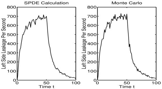
Figure 2: Calculated left leakages per second from time $t=0$ to $t=100$ for one sample path using Monte Carlo and SPDE (10).

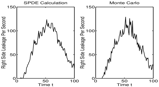
Figure 3: Calculated right leakages per second from time $t=0$ to $t=100$ for one sample path using Monte Carlo and SPDE (10).

The second problem involves neutrons slowing down in a homogeneous medium. It is assumed that at time $t=0.0$, there are 0 neutrons with energy between 0 eV and 10 eV and 400 neutrons with energy between 10 eV and 20 eV. Also, there is present a constant source, $Q(E)$, of neutrons where $Q(E)=\left\{\begin{array}[]{ll}22\;\;\text{for}\;\;10\leq E\leq 20\\ 0\;\;\text{for}\;\;0\leq E\leq 10.\end{array}\right.$ Thus, $\int_{0}^{20}Q(E)\,dE=220$ source neutrons are produced per second. For this problem, the source, $Q(E)$, is assumed to be constant and does not vary randomly. It is furthermore assumed that the total cross section satisfies $v(E)\sigma(E)=1.0\;\;\text{for}\;\;0\leq E\leq 20$, the capture cross section has the form $v(E)\sigma_{c}(E)=\left\{\begin{array}[]{ll}0.1\;\;\text{for}\;\;10\leq E\leq 20\\ 1.0\;\;\text{for}\;\;0\leq E\leq 10\end{array}\right.$ and the scattering cross section has the form $v(E^{\prime})\sigma(E^{\prime})f(E^{\prime},E)=\left\{\begin{array}[]{ll}0.045\;\;\text{for}\;\;10\leq E^{\prime}\leq 20\\ 0.0\;\;\text{for}\;\;0\leq E^{\prime}\leq 10.\end{array}\right.$ For convenience, the product of the speed, $v(E^{\prime})$, with the cross sections are given. The scattering kernel, $\sigma(E^{\prime})f(E^{\prime},E)$, is thus assumed to be piecewise continuous and proportional to $1/\sqrt{E^{\prime}}$ rather than, for example, to $1/E^{\prime}$ such as for a hydrogen-moderated system. Also, notice that the cross sections are consistent in the sense that

$$v(E^{\prime})\sigma(E^{\prime})=v(E^{\prime})\sigma_{c}(E^{\prime})+\int_{0}^{20}v(E^{\prime})\sigma(E^{\prime},E)f(E^{\prime},E)\,dE=1\;\;\;\text{for all}\;\;\;0\leq E^{\prime}\leq 20.$$

Furthermore, for this problem, it can be shown that the mean number of neutrons with energies between 10 eV and 20 eV is equal to 400 for time $t\geq 0$ and the mean number of low-energy neutrons with energies between 0 eV and 10 eV approaches 180 as time $t$ increases. In this problem, the stochastic behavior of the number of neutrons with energies between 0 eV and 10 eV is of interest.

This problem is solved numerically using two independent computational procedures. Specifically, numerical solution of SPDE (12) is compared with Monte Carlo calculations. In the numerical solution of Equation (12), $G=20$ energy groups of equal width $\Delta E=20/G$ are used. Equation (12) is solved using the following stochastic difference equations at discrete times $t_{k}=k\Delta t$ where $\Delta t=0.02$:

$$n_{g,k+1}=n_{g,k}+q_{g,k}\Delta E\Delta t-v_{g}\sigma_{g}n_{g,k}\Delta t+\sum_{g^{\prime}=1}^{G}v_{g^{\prime}}\sigma_{g^{\prime}}f_{g^{\prime},g}n_{g^{\prime},k}\Delta E\Delta t$$ (16)

$$-\sqrt{v_{g}\sigma_{c,g}n_{g,k}\Delta t}\;\eta_{g,k}^{(c)}-\sum_{g^{\prime}=1}^{G}\sqrt{v_{g}\sigma_{g}f_{g,g^{\prime}}n_{g,k}\Delta E\Delta t}\;\eta_{g,g^{\prime},k}^{(tr)}$$

$$+\sum_{g^{\prime}=1}^{G}\sqrt{v_{g^{\prime}}\sigma_{g^{\prime}}f_{g^{\prime},g}n_{g^{\prime},k}\Delta E\Delta t}\;\eta_{g^{\prime},g,k}^{(tr)}$$

where $n_{g,k}\approx n(E_{g},t_{k})$ is the number of neutrons in the $g$th energy group at time $t_{k}=k\Delta t$ and $\sigma_{g}f_{g,g^{\prime}}=\sigma(E_{g})f(E_{g},E_{g^{\prime}})$. Also, $\eta_{g,k}^{(c)},\eta_{g,g^{\prime},k}^{(tr)}\sim\mathcal{N}(0,1)$ are independent normally distributed numbers with mean 0 and variance 1 for each $g,g^{\prime},k$. Difference system (16) is a special case of the stochastic difference system (6). In the Monte Carlo procedure, the neutron population in each energy group is checked at each time step for an absorption, an energy group change, or for an addition from the neutron source. This procedure is continued for each time step until the final time $t=2$.

Calculational results for 100 sample paths using the two independent computational approaches are given in Table 3. The means and standard deviations of the calculated number of neutrons with energies between 0 eV and 10 eV and with energies between 10 eV and 20 eV are given for time $t=2$. The two different computational approaches agree well. In Fig. 4, the calculated number of neutrons with energies between 0 eV and 10 eV are given from time $t=0$ to $t=2$ for one sample path for each calculational method. Again, the results are very similar for the two different calculational procedures.

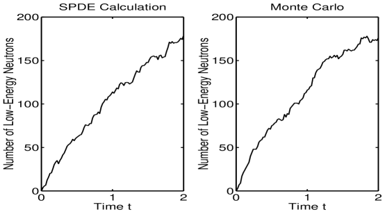
Figure 4: Calculated number of neutrons with energy less than 10.0 from time $t=0$ to $t=2$ for one sample path using Monte Carlo and SPDE (12).

5 Applications

Three possible applications of the stochastic neutron transport equations (8) are in development of new computational methods for solving neutron transport problems, in sensitivity or perturbation analysis, and in testing of computational and analytical methods. Numerical methodology for stochastic partial differential equations is advancing rapidly. It is probable that numerical techniques for solving stochastic neutron transport equations may eventually out-compete Monte Carlo techniques. Stochastic neutron transport equations can also be useful, for example, in perturbation studies to evaluate the effects of small changes in reactor parameters. In addition, solutions of stochastic neutron transport equations can provide independent checks on numerical or analytical approaches such as Monte Carlo methods.

Consider a very simple example of applying stochastic neutron transport equations in a perturbation study. Consider energy-dependent transport in a homogeneous medium with the neutron density given by (12). Assume, for this example, that there is no neutron source and there are no collisions other than capture collisions where the capture cross section varies with time. The stochastic transport equation, for this problem, reduces to:

$$\dfrac{\partial N(E,t)}{\partial t}=-v\sigma_{c}(E,t)N(E,t)-\sqrt{v\sigma_{c}(E,t)N(E,t)}\;\dfrac{\partial^{2}W(E,t)}{\partial E\partial t}.$$ (17)

Suppose that $\sigma_{c}(E,t)$ is perturbed to $\tilde{\sigma}_{c}(E,t)=\sigma_{c}(E,t)+\Delta\sigma_{c}(E,t)$ for $t\geq 0$. We wish to estimate, for the perturbation, the total number of neutrons as well as the change in the variability in this number with time $t$. In particular, if the perturbed neutron density is $N(E,t)+\Delta N(E,t)$, we wish to estimate the change in the total number of neutrons as a function of time, i.e., $\Delta n(t)=\int_{0}^{\infty}\Delta N(E,t)\,dE$. To derive equations for this quantity, let $E_{k}=k\Delta E$ where $\Delta E$ is a small energy interval. Integrating (17) over the interval $[E_{k},E_{k+1}]$, then

$$\dfrac{dn_{k}(t)}{dt}=-v_{k}\sigma_{c}(E_{k},t)n_{k}(t)-\sqrt{v_{k}\sigma_{c}(E_{k},t)n_{k}(t)}\,\dfrac{dW_{k}(t)}{dt}$$ (18)

for $k=0,1,\dots$ where $n_{k}(t)=\int_{E_{k}}^{E_{k+1}}N(E,t)\,dE$. In addition, using Itô’s formula (e.g., [13]),

$$\dfrac{dn_{k}^{2}(t)}{dt}=-2v_{k}\sigma_{c}(E_{k},t)n_{k}^{2}(t)+v_{k}\sigma_{c}(E_{k},t)n_{k}(t)-2n_{k}(t)\sqrt{v_{k}\sigma_{c}(E_{k},t)n_{k}(t)}\,\dfrac{dW_{k}(t)}{dt}.$$ (19)

From (18) and (19), expressions for $E(n_{k}(t))$ and $E(n_{k}^{2}(t))$ are readily obtained and then, $E(n(t))=E(\sum_{k}n_{k}(t))$ and $E(n^{2}(t))=E((\sum_{k}n_{k}(t))^{2})$. Finally, expressions for $E(n(t)+\Delta n(t))-E(n(t))$ and $\text{Var}(n(t)+\Delta n(t))-\text{Var}(n(t))$ are derived as:

$$E(n(t)+\Delta n(t))-E(n(t))=\int_{0}^{\infty}N(E,0)\left(e^{-\int_{0}^{t}v\tilde{\sigma}_{c}(E,s)ds}-e^{-\int_{0}^{t}v\sigma_{c}(E,s)ds}\right)\,dE$$ (20)

and

$$\text{Var}(n(t)+\Delta n(t))-\text{Var}(n(t))=$$

$$\int_{0}^{\infty}N(E,0)e^{-2\int_{0}^{t}v\tilde{\sigma}_{c}(E,s)ds}\left(\int_{0}^{t}v\tilde{\sigma}_{c}(E,s)e^{\int_{0}^{s}v\tilde{\sigma}_{c}(E,r)dr}\,ds\right)\,dE$$

$$-\int_{0}^{\infty}N(E,0)e^{-2\int_{0}^{t}v\sigma_{c}(E,s)ds}\left(\int_{0}^{t}v\sigma_{c}(E,s)e^{\int_{0}^{s}v\sigma_{c}(E,r)dr}\,ds\,\right)dE.$$ (21)

Therefore, using the stochastic neutron transport equation to analyze the effect of the perturbation for this transport process, not only are equations derived for estimating the average effect of the perturbation but equations are also obtained for estimating the change in the variability for the perturbation. Indeed, for this perturbation problem, equations (20) and (21) clearly indicate that the mean change and the change in the variability are both proportional to the initial number of neutrons.

6 Conclusions and Future Directions

Stochastic difference and partial differential equations (SPDEs) are becoming increasingly important in applied mathematics [11, 15, 18, 24]. In the present investigation, stochastic difference equations and an SPDE are derived for neutron transport in a general three-dimensional medium. In the derivation procedure, the deterministic and stochastic terms in the differential equation system are simultaneously derived. First, a stochastic difference system is constructed. Next, an SDE system is derived. Finally, a particular SPDE follows from the SDE system. The stochastic difference equations and the SPDE for the neutron angular densities are given by (6) and (8), respectively. SPDEs for special cases of this equation are given by (10) and (12) for one-dimensional plane geometry and for a homogeneous medium, respectively. The stochastic equations generalize the deterministic neutron transport equations and include random influences due to interactions and sources. Hence, certain random phenomena, such as fluctuations during reactor startup, can be studied using these SPDEs. The stochastic difference equations for neutron transport are solved numerically and compared with independently formulated Monte Carlo methods. The computational results between the two different numerical methods are in good agreement supporting the accuracy of the stochastic neutron transport derivation procedure.

Future work may include appropriately extending the derivations of the present investigation to include the random influence of prompt and delayed neutrons [9, 16, 17]. In addition, stochastic difference equations and an SPDE may be developed to model the random behavior of neutron transport in spherical and cylindrical geometries.

Change $(\Delta n)$	Description	Probability in Time $\Delta t$
$\mu_{x}v_{g}n(x_{i-1},y_{j},z_{k},\mu_{l},\phi_{m},E_{g},t_{p})\Delta t/\Delta x$	In a yz-face $(\mu_{x}>0)$	$1$
$-\mu_{x}v_{g}n(x_{i+1},y_{j},z_{k},\mu_{l},\phi_{m},E_{g},t_{p})\Delta t/\Delta x$	In a yz-face $(\mu_{x}<0)$	$1$
$-|\mu_{x}|v_{g}n(x_{i},y_{j},z_{k},\mu_{l},\phi_{m},E_{g},t_{p})\Delta t/\Delta x$	Out a yz-face	$1$
$\mu_{y}v_{g}n(x_{i},y_{j-1},z_{k},\mu_{l},\phi_{m},E_{g},t_{p})\Delta t/\Delta y$	In a xz-face $(\mu_{y}>0)$	$1$
$-\mu_{y}v_{g}n(x_{i},y_{j+1},z_{k},\mu_{l},\phi_{m},E_{g},t_{p})\Delta t/\Delta y$	In a xz-face $(\mu_{y}<0)$	$1$
$-|\mu_{y}|v_{g}n(x_{i},y_{j},z_{k},\mu_{l},\phi_{m},E_{g},t_{p})\Delta t/\Delta y$	Out a xz-face	$1$
$\mu_{z}v_{g}n(x_{i},y_{j},z_{k-1},\mu_{l},\phi_{m},E_{g},t_{p})\Delta t/\Delta z$	In a xy-face $(\mu_{z}>0)$	$1$
$-\mu_{z}v_{g}n(x_{i},y_{j},z_{k+1},\mu_{l},\phi_{m},E_{g},t_{p})\Delta t/\Delta z$	In a xy-face $(\mu_{z}<0)$	$1$
$-|\mu_{z}|v_{g}n(x_{i},y_{j},z_{k},\mu_{l},\phi_{m},E_{g},t_{p})\Delta t/\Delta z$	Out a xy-face	$1$
$-1$	Capture	$p_{c}$
$-1/\hat{c}$	Transfer out	$p_{tr1}$
$1$	Transfer in	$p_{tr2}$
$1$	Source	$p_{Q}$

Average Number	Standard	Average Number	Standard
Out Left Side	Deviation	Out Right Side	Deviation
704.93 (MC)	23.01 (MC)	100.22 (MC)	9.93 (MC)
694.32 (SPDE)	21.05 (SPDE)	106.75 (SPDE)	7.57 (SPDE)

Average Number	Standard	Average Number	Standard
With Energy	Deviation	With Energy	Deviation
Less Than 10.0		Between 10.0 and 20.0
156.83 (MC)	11.44 (MC)	399.97 (MC)	14.39 (MC)
156.97 (SPDE)	10.28 (SPDE)	400.92 (SPDE)	13.42 (SPDE)

Figure Captions

Fig. 1. A Brownian sheet on $[0,5]\times[0,5]$.

Fig. 2. Calculated left leakages per second from time $t=0$ to $t=100$ for one sample path using Monte Carlo and SPDE (10).

Fig. 3. Calculated right leakages per second from time $t=0$ to $t=100$ for one sample path using Monte Carlo and SPDE (10).

Fig. 4. Calculated number of neutrons with energy less than 10.0 from time $t=0$ to $t=2$ for one sample path using Monte Carlo and SPDE (12).

References

- [1] E. J. Allen, Modeling With Itô Stochastic Differential Equations, Springer, Dordrecht, 2007.
- [2] E. J. Allen, Derivation of Stochastic Partial Differential Equations, Stoch. Anal. Appl. 26(2008), pp. 357-378.
- [3] E. J. Allen, Derivation of Stochastic Partial Differential Equations for Size- and Age-Structured Populations, J. Bio. Dyn. 3(2009), pp. 73-86.
- [4] E. J. Allen, L. J. S. Allen, A. Arciniega, P. E. Greenwood, Construction of equivalent stochastic differential equation models, Stoch. Anal. Appl. 26(2008), pp. 274-297.
- [5] E. J. Allen, S. J. Novosel, Z. Zhang, Finite element and difference approximation of some linear stochastic partial differential equations, Stochastics and Stochastics Reports 64(1998), pp. 117-142.
- [6] L. J. S. Allen, An Introduction to Stochastic Processes with Applications to Biology, Pearson Education Inc., Upper Saddle River, New Jersey, 2003.
- [7] G. I. Bell, Probability distribution of neutrons and precursors in a multiplying assembly, Ann. Phys. 21(1963), pp. 243-283.
- [8] G. I. Bell, On the stochastic theory of neutron transport, Nucl. Sci. and Eng. 21(1965), pp. 390-401.
- [9] G. I. Bell, S. Glasstone, Neutron Transport Theory, Van Nostrand Reinhold Company, New York, 1970.
- [10] E. M. Cabaña, The vibrating string forced by white noise, Z. Wahrscheinlichkeit. 15(1970), pp. 111-130.
- [11] G. Da Prato, L. Tubaro (Eds.), Stochastic Partial Differential Equations and Applications - VII, CRC Press, Taylor & Francis Group, Boca Raton, Florida, 2006.
- [12] J. Duderstadt, W. Martin, Transport Theory, John Wiley and Sons, New York, 1979.
- [13] T. C. Gard, Introduction to Stochastic Differential Equations, Marcel Decker, New York, 1987.
- [14] D. T. Gillespie, The chemical Langevin equation, J. Chem. Phys. 113(2000), pp. 297-306.
- [15] M. Gunzburger, Numerical methods for stochastic PDEs, SIAM News 40(2007), pg. 3.
- [16] J. G. Hayes and E. J. Allen, Stochastic point-kinetics equations in nuclear reactor dynamics, Ann. Nucl. Eng. 32(2005), pp. 572-587.
- [17] D. L. Hetrick, Dynamics of Nuclear Reactors, The University of Chicago Press, Chicago, 1971.
- [18] H. Holden, B. Øksendal, J. Ubøe, T. Zhang, Stochastic Partial Differential Equations: A Modeling, White Noise Functional Approach, Birhäuser, Boston, Massachusetts, 1996.
- [19] Y. Kitamura, L. Pál, I. Pázit, A. Yamamoto, Y. Yamane, Some properties of zero power noise in a time-varying medium with delayed neutrons, Ann. Nucl. Eng. 35(2008), pp. 1621-1627.
- [20] P. E. Kloeden, E. Platen, Numerical Solution of Stochastic Differential Equations, Springer-Verlag, New York, 1992.
- [21] P. E. Kloeden, E. Platen, H. Schurz, Numerical Solution of SDE Through Computer Experiments, Springer, Berlin, 1994.
- [22] E. E. Lewis, W. F. Miller, Computational Methods of Neutron Transport, John Wiley, New York, 1984.
- [23] L. Pál, I. Pázit, Theory of neutron noise in a temporally fluctuating multiplying medium, Nucl. Sci. Eng. 155(2007), pp. 425-440.
- [24] H. Schurz, Nonlinear stochastic wave equations in with power-law nonlinearity and additive space-time noise, Contemp. Math. 440(2007), pp. 223-242.
- [25] W. D. Sharp and E. J. Allen, Stochastic neutron transport equations for rod and plane geometries, Ann. Nucl. Eng. 27(2000), 99-116.
- [26] N. G. van Kampen, Stochastic Processes in Physics and Chemistry, Elsevier Science B. V., Amsterdam, The Netherlands, 1992.
- [27] J. B. Walsh, An Introduction to Stochastic Partial Differential Equations, in Lecture Notes in Mathematics, Vol. 1180, A. Dold, B. Eckmann, eds., Springer-Verlag, Berlin, 1986, pp. 265-439.
- [28] M. M. R. Williams, E. W. Larsen, Neutron transport in spatially random media: eigenvalue problems, Nucl. Sci. Eng. 139(2001), pp. 66-77.
- [29] M. M. R. Williams, The effect of random geometry on the criticality of a multiplying system IV: transport theory, Nucl. Sci. Eng. 143(2003), pp. 1-18.
TABLE 1
Possible Changes in the Number for Time