Linearized stability analysis of gravastars in noncommutative geometry

Abstract

In this work, we find exact gravastar solutions in the context of noncommutative geometry, and explore their physical properties and characteristics. The energy density of these geometries is a smeared and particle-like gravitational source, where the mass is diffused throughout a region of linear dimension $\sqrt{\alpha}$ due to the intrinsic uncertainty encoded in the coordinate commutator. These solutions are then matched to an exterior Schwarzschild spacetime. We further explore the dynamical stability of the transition layer of these gravastars, for the specific case of $\beta=M^{2}/\alpha<1.9$, where $M$ is the black hole mass, to linearized spherically symmetric radial perturbations about static equilibrium solutions. It is found that large stability regions exist and, in particular, located sufficiently close to where the event horizon is expected to form.

I Introduction

Recently, an alternative picture for the final state of gravitational collapse has emerged Mazur . The latter, denoted as a gravastar (gravitational vacuum star), consists of an interior compact object matched to an exterior Schwarzschild vacuum spacetime, at or near where the event horizon is expected to form. Therefore, these alternative models do not possess a singularity at the origin and have no event horizon, as its rigid surface is located at a radius slightly greater than the Schwarzschild radius. More specifically, the gravastar picture, proposed by Mazur and Mottola Mazur , has an effective phase transition at/near where the event horizon is expected to form, and the interior is replaced by a de Sitter condensate. This new emerging picture consisting of a compact object resembling ordinary spacetime, in which the vacuum energy is much larger than the cosmological vacuum energy, is also denoted as a “dark energy star” Chapline . In fact, a wide variety of gravastar models have been considered in the literature gravastar1 ; gravastar2 and their observational signatures have also been explored gravastar3 . In this work, we consider a further extension of the gravastar picture in the context of noncommutative geometry. The dynamical stability of the transition layer of these gravastars to linearized spherically symmetric radial perturbations about static equilibrium solutions is also explored. The analysis of thin shells linear-thinshell and the respective linearized stability analysis of thin shells has been recently extensively considered in the literature, and we refer the reader to Refs. linearstability ; linear-WH for details.

In the context of noncommutative geometry, an interesting development of string/M-theory has been the necessity for spacetime quantization, where the spacetime coordinates become noncommuting operators on a $D$-brane Witten . The noncommutativity of spacetime is encoded in the commutator $\left[\mathbf{x}^{\mu},\mathbf{x}^{\nu}\right]=i\,\theta^{\mu\nu}$, where $\theta^{\mu\nu}$ is an antisymmetric matrix which determines the fundamental discretization of spacetime. It has also been shown that noncommutativity eliminates point-like structures in favor of smeared objects in flat spacetime Smailagic:2003yb . Thus, one may consider the possibility that noncommutativity could cure the divergences that appear in general relativity. The effect of the smearing is mathematically implemented with a substitution of the Dirac-delta function by a Gaussian distribution of minimal length $\sqrt{\alpha}$. In particular, the energy density of a static and spherically symmetric, smeared and particle-like gravitational source has been considered in the following form Nicolini:2005vd

$$\rho_{\alpha}(r)=\frac{M}{(4\pi\alpha)^{3/2}}\;\mathrm{exp}\left(-\frac{r^{2}}{4\alpha}\right)\,,$$ (1)

where the mass $M$ is diffused throughout a region of linear dimension $\sqrt{\alpha}$ due to the intrinsic uncertainty encoded in the coordinate commutator.

The Schwarzschild metric is modified when a non-commutative spacetime is taken into account Nicolini:2005vd ; Esposito . The solution obtained is described by the following spacetime metric

$$ds^{2}=-f(r)\,dt^{2}+\frac{dr^{2}}{f(r)}+r^{2}\,(d\theta^{2}+\sin^{2}{\theta}\,d\phi^{2})\,,$$ (2)

with $f(r)=1-2m(r)/r$, where the mass function is defined as

$$m(r)=\frac{2M}{\sqrt{\pi}}\gamma\left(\frac{3}{2},\frac{r^{2}}{4\alpha}\right)\,,$$ (3)

and

$$\gamma\left(\frac{3}{2},\frac{r^{2}}{4\alpha}\right)=\int\limits_{0}^{r^{2}/4\alpha}dt\sqrt{t}\exp\left(-t\right)$$ (4)

is the lower incomplete gamma function Nicolini:2005vd . The classical Schwarzschild mass is recovered in the limit $r/\sqrt{\alpha}\rightarrow\infty$. It was shown that the coordinate noncommutativity cures the usual problems encountered in the description of the terminal phase of black hole evaporation. More specifically, it was found that the evaporation end-point is a zero temperature extremal black hole and there exist a finite maximum temperature that a black hole can reach before cooling down to absolute zero. The existence of a regular de Sitter at the origin’s neighborhood was also shown, implying the absence of a curvature singularity at the origin. Recently, further research on noncommutative black holes has been undertaken, with new solutions found providing smeared source terms for charged and higher dimensional cases newNCGbh . Furthermore, exact solutions of semi-classical wormholes Garattini2 in the context of noncommutative geometry were found Garattini1 , and their physical properties and characteristics were analyzed.

This paper is outlined in the following manner. In Section II, we present the generic structure equations of gravastars, and specify the mass function in the context of noncommutative geometry. In Section III, the linearized stability analysis procedure is briefly outlined, and the stability regions of the transition layer of gravastars are determined. Finally in Section IV, we conclude. We adopt the convention $G=c=1$ throughout this work.

II Structure equations of gravastars in noncommutative geometry

Consider the interior spacetime, without a loss of generality, given by the following metric, in curvature coordinates

$$ds^{2} = -e^{2\Phi(r)}\,dt^{2}+\frac{dr^{2}}{1-2m(r)/r}+r^{2}\,d\Omega^{2}\,,$$ (5)

where $d\Omega^{2}=(d\theta^{2}+\sin^{2}{\theta}\,d\phi^{2})$; $\Phi(r)$ and $m(r)$ are arbitrary functions of the radial coordinate, $r$. The function $m(r)$ is the quasi-local mass, and is denoted as the mass function.

The Einstein field equation, $G_{\mu\nu}=8\pi T_{\mu\nu}$ provides the following relationships

$$m^{\prime} = 4\pi r^{2}\rho\,,$$ (6)

$$\Phi^{\prime} = \frac{m+4\pi r^{3}p_{r}}{r(r-2m)}\,,$$ (7)

$$p_{r}^{\prime} = -\frac{(\rho+p_{r})(m+4\pi r^{3}p_{r})}{r(r-2m)}+\frac{2}{r}(p_{t}-p_{r})\,,$$ (8)

where the prime denotes a derivative with respect to the radial coordinate. $\rho(r)$ is the energy density, $p_{r}(r)$ is the radial pressure, and $p_{t}(r)$ is the tangential pressure. Equation (8) corresponds to the anisotropic pressure Tolman-Oppenheimer-Volkoff (TOV) equation. The factor $\Phi^{\prime}(r)$ may be considered the “gravity profile” as it is related to the locally measured acceleration due to gravity, through the following relationship gravastar2 : ${\cal A}=\sqrt{1-2m(r)/r}\,\Phi^{\prime}(r)$. The convention used is that $\Phi^{\prime}(r)$ is positive for an inwardly gravitational attraction, and negative for an outward gravitational repulsion.

Using the equation of state, $p_{r}=-\rho$, and taking into account the field equations (6) and (7), we have the following relationship

$$\Phi^{\prime}(r)=\frac{m-rm^{\prime}}{r\,\left(r-2m\right)}\,,$$ (9)

which provides the solution given by

$$\Phi(r)=\frac{1}{2}\ln\left[1-\frac{2m(r)}{r}\right]\,.$$ (10)

One now has at hand three equations, namely, the field Eqs. (6)-(8), with four unknown functions of $r$, i.e., $\rho(r)$, $p_{r}(r)$, $p_{t}(r)$, and $m(r)$. We shall consider the approach by choosing a specific choice for a physically reasonable mass function $m(r)$, thus closing the system.

In this context, we are interested in the noncommutative geometry inspired mass function given by Eq. (3). The latter is reorganized into the following form

$$m(r)=\frac{2M}{\sqrt{\pi}}\gamma\left(\frac{3}{2},\beta\left(\frac{r}{2M}\right)^{2}\right)\,,$$ (11)

where $\beta$ is defined as $\beta=M^{2}/\alpha$.

Note that three cases need to be analyzed Nicolini:2005vd :

a)

If $\beta<1.9$, no roots are present;

b)

If $\beta>1.9$, we have two roots, $r_{-}$ and $r_{+}$, with $r_{+}>r_{-}$;

c)

If $\beta=1.9$, we have $r_{+}=r_{-}$, which may be interpreted as an extreme situation, such as the extreme Reissner-Nordström metric.

The function $f(r)=(1-2m(r)/r)$ is depicted in Fig. 1 for these three cases for the following values $\beta=1.5$, $\beta=1.9$ and $\beta=3.5$, respectively. Note that all the roots lie within the Schwarzschild radius $r_{b}=2M$, where $M$ is the total mass of the system.

Figure 1: The function $f(r)=(1-2m(r)/r)$ is depicted for the three cases with the following values $\beta=1.5$, $\beta=1.9$ and $\beta=3.5$, respectively.

III Linearized stability of gravastars in noncommutative geometry

III.1 Junction interface and surface stresses

We shall model specific gravastar geometries by matching an interior gravastar geometry, given by Eq. (5), where the metric functions are given by Eqs. (10) and (11), with an exterior Schwarzschild solution

$$ds^{2} = -\left(1-\frac{2M}{r}\right)\,dt^{2}+\left(1-\frac{2M}{r}\right)^{-1}\,dr^{2}$$ (12)

$$+r^{2}\,(d\theta^{2}+\sin^{2}{\theta}\,d\phi^{2})\,,$$

at a junction interface $\Sigma$, situated outside the event horizon, $a>r_{b}=2M$. We emphasize that the larger root $r_{+}$ lies inside the Schwarzschild event horizon. Thus, in this work we are only interested in the case of $\beta<1.9$, which corresponds to the absence of event horizons for the inner solution.

Consider the junction surface $\Sigma$ as a timelike hypersurface defined by the parametric equation of the form $f(x^{\mu}(\xi^{i}))=0$. $\xi^{i}=(\tau,\theta,\phi)$ are the intrinsic coordinates on $\Sigma$, where $\tau$ is the proper time on the hypersurface. The three basis vectors tangent to $\Sigma$ are given by $e_{(i)}=\partial/\partial\xi^{i}$, with the following components $e^{\mu}_{(i)}=\partial x^{\mu}/\partial\xi^{i}$. The induced metric on the junction surface is then provided by the scalar product $g_{ij}=e_{(i)}\cdot e_{(j)}=g_{\mu\nu}e^{\mu}_{(i)}e^{\nu}_{(j)}$. Thus, the intrinsic metric to $\Sigma$ is given by

$$ds^{2}_{\Sigma}=-d\tau^{2}+a^{2}\,(d\theta^{2}+\sin^{2}{\theta}\,d\phi^{2})\,.$$ (13)

Note that the junction surface, $r=a$, is situated outside the event horizon, i.e., $a>r_{b}$, to avoid a black hole solution, and we are only interested in the case of $\beta<1.9$, of Eq. (11), as emphasized above.

For the specific cases considered in this work, namely, the interior and exterior spacetimes given by Eqs. (5) and (12), respectively, the four-velocity of the junction surface $x^{\mu}(\tau,\theta,\phi)=(t(\tau),a(\tau),\theta,\phi)$ is given by

$$U_{\pm}^{\mu}=\left(\frac{dt}{d\tau},\frac{da}{d\tau},0,0\right)=\left(\frac{\sqrt{1-\frac{2m_{\pm}}{a}+\dot{a}^{2}}}{1-\frac{2m_{\pm}}{a}},\dot{a},0,0\right),$$ (14)

where the $(\pm)$ superscripts correspond to the exterior and interior spacetimes, respectively, so that $m_{\pm}$ are defined as $m_{-}=m(a)$ and $m_{+}=M$, respectively.

The unit normal $4-$vector, $n^{\mu}$, to $\Sigma$ is defined as

$$n_{\mu}=\pm\,\left|g^{\alpha\beta}\,\frac{\partial f}{\partial x^{\alpha}}\,\frac{\partial f}{\partial x^{\beta}}\right|^{-1/2}\;\frac{\partial f}{\partial x^{\mu}}\,,$$ (15)

with $n_{\mu}\,n^{\mu}=+1$ and $n_{\mu}e^{\mu}_{(i)}=0$. The Israel formalism requires that the normals point from the interior spacetime to the exterior spacetime Israel . Thus, for the interior and exterior spacetimes given by the metrics (5) and (12), respectively, the normals may be determined from Eq. (15), or from the contractions $U^{\mu}n_{\mu}=0$ and $n^{\mu}n_{\mu}=+1$, and are provided by

$$n^{\pm}_{\mu}=\left(-\dot{a},\frac{\sqrt{1-\frac{2m_{\pm}}{a}+\dot{a}^{2}}}{1-\frac{2m_{\pm}}{a}},0,0\right)\,,$$ (16)

respectively, with $m_{\pm}$ defined as $m_{-}=m(a)$ and $m_{+}=M$, as before.

The extrinsic curvature is defined as $K_{ij}=n_{\mu;\nu}e^{\mu}_{(i)}e^{\nu}_{(j)}$. Differentiating $n_{\mu}e^{\mu}_{(i)}=0$ with respect to $\xi^{j}$, we have $n_{\mu}\frac{\partial^{2}x^{\mu}}{\partial\xi^{i}\,\partial\xi^{j}}=-n_{\mu,\nu}\,\frac{\partial x^{\mu}}{\partial\xi^{i}}\frac{\partial x^{\nu}}{\partial\xi^{j}}$, so that the extrinsic curvature is finally given by

$$K_{ij}^{\pm}=-n_{\mu}\left(\frac{\partial^{2}x^{\mu}}{\partial\xi^{i}\,\partial\xi^{j}}+\Gamma^{\mu\pm}_{\;\;\alpha\beta}\;\frac{\partial x^{\alpha}}{\partial\xi^{i}}\,\frac{\partial x^{\beta}}{\partial\xi^{j}}\right)\,.$$ (17)

Note that, in general, $K_{ij}$ is not continuous across $\Sigma$, so that for notational convenience, the discontinuity in the extrinsic curvature is defined as $\kappa_{ij}=K_{ij}^{+}-K_{ij}^{-}$.

Taking into account the interior spacetime metric (5) and the Schwarzschild solution (12), the non-trivial components of the extrinsic curvature are given by

$$K^{\tau\;+}_{\;\;\tau} = \frac{\frac{M}{a^{2}}+\ddot{a}}{\sqrt{1-\frac{2M}{a}+\dot{a}^{2}}}\;,$$ (18)

$$K^{\tau\;-}_{\;\;\tau} = \frac{\frac{m}{a^{2}}-\frac{m^{\prime}}{a}+\ddot{a}}{\sqrt{1-\frac{2m(a)}{a}+\dot{a}^{2}}}\;,$$ (19)

and

$$K^{\theta\;+}_{\;\;\theta} = \frac{1}{a}\sqrt{1-\frac{2M}{a}+\dot{a}^{2}}\;,$$ (20)

$$K^{\theta\;-}_{\;\;\theta} = \frac{1}{a}\sqrt{1-\frac{2m(a)}{a}+\dot{a}^{2}}\;,$$ (21)

respectively.

The Einstein equations may be written in the following form,

$$S^{i}_{\;j}=-\frac{1}{8\pi}\,(\kappa^{i}_{\;j}-\delta^{i}_{\;j}\kappa^{k}_{\;k})\,,$$ (22)

denoted as the Lanczos equations, where $S^{i}_{\;j}$ is the surface stress-energy tensor on $\Sigma$. Considerable simplifications occur due to spherical symmetry, namely $\kappa^{i}_{\;j}={\rm diag}\left(\kappa^{\tau}_{\;\tau},\kappa^{\theta}_{\;\theta},\kappa^{\theta}_{\;\theta}\right)$. The surface stress-energy tensor may be written in terms of the surface energy density, $\sigma$, and the surface pressure, ${\cal P}$, as $S^{i}_{\;j}={\rm diag}(-\sigma,{\cal P},{\cal P})$. Thus, the Lanczos equation, Eq. (22), then provide us with the following expressions for the surface stresses

$$\sigma = -\frac{1}{4\pi a}\left(\sqrt{1-\frac{2M}{a}+\dot{a}^{2}}-\sqrt{1-\frac{2m}{a}+\dot{a}^{2}}\,\right),$$ (23)

$${\cal P} = \frac{1}{8\pi a}\Bigg{[}\frac{1-\frac{M}{a}+\dot{a}^{2}+a\ddot{a}}{\sqrt{1-\frac{2M}{a}+\dot{a}^{2}}}-\frac{1-\frac{m}{a}-m^{\prime}+\dot{a}^{2}+a\ddot{a}}{\sqrt{1-\frac{2m}{a}+\dot{a}^{2}}}\,\Bigg{]}\,.$$ (24)

We also use the conservation identity given by $S^{i}_{j|i}=\left[T_{\mu\nu}e^{\mu}_{(j)}n^{\nu}\right]^{+}_{-}$, where $[X]^{+}_{-}$ denotes the discontinuity across the surface interface, i.e., $[X]^{+}_{-}=X^{+}|_{\Sigma}-X^{-}|_{\Sigma}$. The momentum flux term in the right hand side corresponds to the net discontinuity in the momentum flux $F_{\mu}=T_{\mu\nu}\,U^{\nu}$ which impinges on the shell. The conservation identity is a statement that all energy and momentum that plunges into the thin shell, gets caught by the latter and converts into conserved energy and momentum of the surface stresses of the junction.

Note that $S^{i}_{\tau|i}=-\left[\dot{\sigma}+2\dot{a}(\sigma+{\cal P})/a\right]$, so that the conservation identity provides us with

$$\sigma^{\prime}=-\frac{2}{a}\,(\sigma+{\cal P})\,.$$ (25)

This relationship will be used in the linearized stability analysis considered below.

III.2 Linearized stability analysis

Using the surface mass of the thin shell $m_{s}=4\pi a^{2}\sigma$, Eq. (25) can be rearranged to provide the following relationship

$$\left(\frac{m_{s}}{2a}\right)^{\prime\prime}=\Upsilon-4\pi\sigma^{\prime}\eta\,,$$ (26)

with the parameter $\eta$ defined as $\eta={\cal P}^{\prime}/\sigma^{\prime}$, and $\Upsilon$ given by

$$\Upsilon\equiv\frac{4\pi}{a}\,(\sigma+{\cal P})\,.$$ (27)

Equation (26) will play a fundamental role in determining the stability regions of the respective solutions. Note that $\eta$ is used as a parametrization of the stable equilibrium, so that there is no need to specify a surface equation of state. The parameter $\sqrt{\eta}$ is normally interpreted as the speed of sound, so that one would expect that $0<\eta\leq 1$, based on the requirement that the speed of sound should not exceed the speed of light. We refer the reader to Refs. linear-WH for further discussions on the respective physical interpretation of $\eta$ lying outside the range $0<\eta\leq 1$.

Equation (23) may be rearranged to provide the thin shell’s equation of motion given by

$$\dot{a}^{2}+V(a)=0\,.$$ (28)

The potential is given by

$$V(a)=F(a)-\left[\frac{m_{s}(a)}{2a}\right]^{2}-\left[\frac{aG(a)}{m_{s}(a)}\right]^{2}\,.$$ (29)

where, for notational convenience, the factors $F(a)$ and $G(a)$ are defined as

$$F(a)=1-\frac{m(a)+M}{a}\quad{\rm and}\quad G(a)=\frac{M-m(a)}{a}\,.$$ (30)

Linearizing around a stable solution situated at $a_{0}$, we consider a Taylor expansion of $V(a)$ around $a_{0}$ to second order, given by

$$V(a) = V(a_{0})+V^{\prime}(a_{0})(a-a_{0})$$ (31)

$$+\frac{1}{2}V^{\prime\prime}(a_{0})(a-a_{0})^{2}+O\left[(a-a_{0})^{3}\right]\,.$$

Evaluated at the static solution, at $a=a_{0}$, we verify that $V(a_{0})=0$ and $V^{\prime}(a_{0})=0$. From the condition $V^{\prime}(a_{0})=0$, one extracts the following useful equilibrium relationship

$$\Gamma\equiv\left(\frac{m_{s}}{2a_{0}}\right)^{\prime}=\left(\frac{a_{0}}{m_{s}}\right)\left[F^{\prime}-2\left(\frac{a_{0}G}{m_{s}}\right)\left(\frac{a_{0}G}{m_{s}}\right)^{\prime}\right]\,,$$ (32)

which will be used in determining the master equation, responsible for dictating the stable equilibrium configurations.

The solution is stable if and only if $V(a)$ has a local minimum at $a_{0}$ and $V^{\prime\prime}(a_{0})>0$ is verified. Thus, from the latter stability condition, one may deduce the master equation, given by

$$\eta_{0}\,\frac{d\sigma^{2}}{da}\Big{|}_{a_{0}}>\Theta\,,$$ (33)

by using Eq. (26), where $\eta_{0}=\eta(a_{0})$ and $\Theta$, for notational simplicity, is defined by

$$\Theta\equiv\frac{1}{2\pi}\left[\sigma\Upsilon+\frac{1}{2\pi a_{0}}\left(\Gamma^{2}-\Psi\right)\right]\,,$$ (34)

with

$$\Psi=\frac{F^{\prime\prime}}{2}-\left[\left(\frac{aG}{m_{s}}\right)^{\prime}\right]^{2}-\left(\frac{aG}{m_{s}}\right)\left(\frac{aG}{m_{s}}\right)^{\prime\prime}\,.$$ (35)

Now, from the master equation we find that the stable equilibrium regions are dictated by the following inequalities

$$\eta_{0} > \Omega,\qquad{\rm if}\qquad\frac{d\sigma^{2}}{da}\Big{|}_{a_{0}}>0\,,$$ (36)

$$\eta_{0} < \Omega,\qquad{\rm if}\qquad\frac{d\sigma^{2}}{da}\Big{|}_{a_{0}}<0\,,$$ (37)

with the definition

$$\Omega\equiv\Theta\left(\frac{d\sigma^{2}}{da}\Big{|}_{a_{0}}\right)^{-1}\,.$$ (38)

III.3 Stability regions

We now determine the stability regions dictated by the inequalities (36)-(37). In the specific cases that follow, the explicit form of $\Omega$ is extremely messy, so that we find it more instructive to show the stability regions graphically.

For the case of interest under consideration, namely, $\beta<1.9$, we verify that $d\sigma^{2}/da|_{a_{0}}<0$, so that the stability regions are dictated by inequality (37). The latter is shown graphically in Fig. 2, for the specific case of $\beta=1.0$.

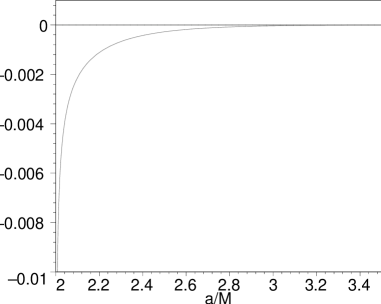
Figure 2: Sign of $(d\sigma^{2}/da)|_{a_{0}}$, for $\beta=1$, which corresponds to the absence of horizons.

Considering the case of $\beta=1.0$, the respective stability regions are given by the plot depicted below the curve in Fig. 3. Note the existence of large stability regions sufficiently close to the event horizon. For this case, the stability regions decrease for increasing $a$, and increases again as $a$ increases.

The above analysis shows that stable configurations of the surface layer, located sufficiently near to where the event horizon is expected to form, do indeed exist. Therefore, considering these models, one may conclude that the exterior geometry of a dark energy star would be practically indistinguishable from a black hole.

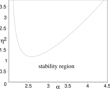
Figure 3: Stability plot for $\beta=1$, which corresponds to the absence of horizons; we have defined $\alpha=a/M$.

IV Conclusion

In this work, we have found exact gravastar solutions in the context of noncommutative geometry, and briefly explored their physical properties and characteristics. The energy density of these geometries is a smeared and particle-like gravitational source, where the mass is diffused throughout a region of linear dimension $\sqrt{\alpha}$ due to the intrinsic uncertainty encoded in the coordinate commutator.

We further explored the dynamical stability of the transition layer of these dark energy stars to linearized spherically symmetric radial perturbations about static equilibrium solutions. It was found that large stability regions do exist, which are located sufficiently close to where the event horizon is expected to form, so that it would be difficult to distinguish the exterior geometry of the gravastars, analyzed in this work, from a black hole.

References

- (1) P. O. Mazur and E. Mottola, “Gravitational Condensate Stars: An Alternative to Black Holes,” [arXiv:gr-qc/0109035]; P. O. Mazur and E. Mottola, “Dark energy and condensate stars: Casimir energy in the large,” [arXiv:gr-qc/0405111]; P. O. Mazur and E. Mottola, “Gravitational Vacuum Condensate Stars,” Proc. Nat. Acad. Sci. 111, 9545 (2004) [arXiv:gr-qc/0407075]; G. Chapline, E. Hohlfeld, R. B. Laughlin and D. I. Santiago, Int. J. Mod. Phys. A 18 3587-3590 (2003).
- (2) G. Chapline, “Dark energy stars,” [arXiv:astro-ph/0503200]; F. S. N. Lobo, Class. Quant. Grav. 23, 1525 (2006).
- (3) M. Visser and D. L. Wiltshire, Class. Quantum Grav. 21, 1135 (2004); B. M. N. Carter, Class. Quantum Grav. 22, 4551 (2005); P. Rocha, R. Chan, M. F. A. da Silva and A. Wang, JCAP 0811, 010 (2008); C. Cattoen, T. Faber and M. Visser, Class. Quantum Grav. 22, 4189 (2005); A. DeBenedictis, D. Horvat, S. Ilijic, S. Kloster and K. S. Viswanathan, Class. Quant. Grav. 23, 2303 (2006); F. S. N. Lobo and A. V. B. Arellano, Class. Quant. Grav. 24, 1069 (2007); N. Bilic, G. B. Tupper and R. D. Viollier, JCAP 0602, 013 (2006); A. DeBenedictis, R. Garattini and F. S. N. Lobo, Phys. Rev. D 78, 104003 (2008); O. Bertolami and J. Paramos, Phys. Rev. D 72, 123512 (2005);
- (4) F. S. N. Lobo, Phys. Rev. D 75, 024023 (2007).
- (5) A. E. Broderick and R. Narayan, Class. Quantum Grav. 24, 659 (2007); C. B. M. H. Chirenti and L. Rezzolla, Class. Quantum Grav. 24, 4191 (2007); D. Horvat and S. Ilijic, Class. Quantum Grav. 24, 5637 (2007); V. Cardoso, P. Pani, M. Cadoni and M. Cavaglia, Phys. Rev. D 77, 124044 (2008); C. B. M. H. Chirenti and L. Rezzolla, Phys. Rev. Dbf 78, 084011 (2008); D. Horvat, S. Ilijic and A. Marunovic, Class. Quantum Grav. 26, 025003 (2009); B. V. Turimov, B. J. Ahmedov and A. A. Abdujabbarov, MPLA, in press, arXiv:0902.0217 (2009); T. Harko, Z. Kovacs and F. S. N. Lobo, Class. Quant. Grav. 26, 215006 (2009).
- (6) J. P. S. Lemos, F. S. N. Lobo and S. Quinet de Oliveira, Phys. Rev. D 68, 064004 (2003); F. S. N. Lobo, Phys. Rev. D 75, 024023 (2007); S. Sushkov, Phys. Rev. D 71, 043520 (2005); F. S. N. Lobo, Phys. Rev. D 71, 084011 (2005); E. F. Eiroa, Phys. Rev. D 78, 024018 (2008); F. S. N. Lobo, Class. Quant. Grav. 21, 4811 (2004); F. S. N. Lobo, Gen. Rel. Grav. 37, 2023 (2005); J. P. S. Lemos and F. S. N. Lobo, Phys. Rev. D 69, 104007 (2004); F. S. N. Lobo, arXiv:0710.4474 [gr-qc].
- (7) P. R. Brady, J. Louko and E. Poisson, Phys. Rev. D 44, 1891 (1991); M. Ishak and K. Lake, Phys. Rev. D 65, 044011 (2002); E. F. Eiroa and G. E. Romero Gen. Rel. Grav. 36 651-659 (2004); F. S. N. Lobo and P. Crawford, Class. Quant. Grav. 22, 4869 (2005); F. S. N. Lobo, Phys. Rev. D 71, 124022 (2005); E. F. Eiroa and C. Simeone, Phys. Rev. D 70, 044008 (2004); E. F. Eiroa and C. Simeone, Phys. Rev. D 71, 127501 (2005); M. Thibeault, C. Simeone and E. F. Eiroa, Gen. Rel. Grav. 38, 1593 (2006); F. Rahaman, M. Kalam and S. Chakraborty, Gen. Rel. Grav. 38, 1687 (2006); C. Bejarano, E. F. Eiroa and C. Simeone, Phys. Rev. D 75, 027501 (2007); F. Rahaman, M. Kalam and S. Chakraborty, Int. J. Mod. Phys. D 16, 1669 (2007); E. F. Eiroa and C. Simeone, Phys. Rev. D 76, 024021 (2007); F. Rahaman, M. Kalam, K. A. Rahman and S. Chakraborty, Gen. Rel. Grav. 39, 945 (2007); M. G. Richarte and C. Simeone, [arXiv:0711.2297 [gr-qc]].
- (8) E. Poisson and M. Visser, Phys. Rev. D 52 7318 (1995); F. S. N. Lobo and P. Crawford, Class. Quant. Grav. 21, 391 (2004).
- (9) E. Witten, Nucl. Phys. B 460, 335 (1996); N. Seiberg and E. Witten, JHEP 9909, 032 (1999).
- (10) A. Smailagic and E. Spallucci, J. Phys. A 36, L467 (2003).
- (11) P. Nicolini, A. Smailagic and E. Spallucci, Phys. Lett. B 632, 547 (2006).
- (12) E. Di Grezia, G. Esposito and G. Miele, J.Phys.A 41, 164063 (2008).
- (13) R. Casadio and P. Nicolini, arXiv:0809.2471 [hep-th]; P. Nicolini, arXiv:0807.1939 [hep-th]; E. Spallucci, A. Smailagic and P. Nicolini, arXiv:0801.3519 [hep-th]; S. Ansoldi, P. Nicolini, A. Smailagic and E. Spallucci, Phys. Lett. B 645, 261 (2007); P. Nicolini, J. Phys. A 38, L631 (2005).
- (14) R. Garattini and F. S. N. Lobo, Class. Quant. Grav. 24, 2401 (2007).
- (15) R. Garattini and F. S. N. Lobo, Phys. Lett. B 671, 146 (2009).
- (16) K. Lanczos, Ann. Phys. (Leipzig) 74, 518 (1924); G. Darmois, Fasticule XXV ch V (Gauthier-Villars, Paris, France, 1927); W. Israel, Nuovo Cimento 44B, 1 (1966); and corrections in ibid. 48B, 463 (1966); A. Papapetrou and A. Hamoui, Ann. Inst. Henri Poincaré 9, 179 (1968).