How Much Multiuser Diversity is Required for Energy Limited Multiuser Systems?

Abstract

Multiuser diversity (MUDiv) is one of the central concepts in multiuser (MU) systems. In particular, MUDiv allows for scheduling among users in order to eliminate the negative effects of unfavorable channel fading conditions of some users on the system performance. Scheduling, however, consumes energy (e.g., for making users’ channel state information available to the scheduler). This extra usage of energy, which could potentially be used for data transmission, can be very wasteful, especially if the number of users is large. In this paper, we answer the question of how much MUDiv is required for energy limited MU systems. Focusing on uplink MU wireless systems, we develop MU scheduling algorithms which aim at maximizing the MUDiv gain. Toward this end, we introduce a new realistic energy model which accounts for scheduling energy and describes the distribution of the total energy between scheduling and data transmission stages. Using the fact that such energy distribution can be controlled by varying the number of active users, we optimize this number by either (i) minimizing the overall system bit error rate (BER) for a fixed total energy of all users in the system or (ii) minimizing the total energy of all users for fixed BER requirements. We find that for a fixed number of available users, the achievable MUDiv gain can be improved by activating only a subset of users. Using asymptotic analysis and numerical simulations, we show that our approach benefits from MUDiv gains higher than that achievable by generic greedy access algorithm, which is the optimal scheduling method for energy unlimited systems.

I Introduction

In wireless systems, unfavorable channel conditions remain the main hinderance to achieving desirable system throughput or bit error rate (BER). To overcome this problem in multiuser (MU) wireless systems, resource scheduling strategies, which use channel fading conditions as an opportunistic resource, have been proposed [1, 2]. Using the so-called opportunistic transmission, advanced scheduling strategies along with closed-loop designs [3, 4] have been developed in the literature (see [2, 5, 6] and references therein). The gain obtained by such opportunistic transmission methods is known as multiuser diversity (MUDiv) gain.

For multi-point–to–point single–input single–output (SISO) wireless systems, the MUDiv gain was first studied in [1]. The information theoretic results have shown that based on the optimal transmit power control, the overall system throughput can be maximized by allowing only the ‘best’ user in a system to transmit at each time slot. For downlink MU systems, the MUDiv has been recognized as an effective method of improving the system performance measures such as spectral efficiency and quality of service over multipath fading channels [2]. As a result, MUDiv approaches have been adopted in commercial systems, e.g., systems based on orthogonal frequency division multiple access (OFDMA) [7].

Toward improving the MUDiv gain, various system performance measures and their tradeoffs have been considered, as well as various algorithms have been developed [8]–[13]. In [8], the problem of multiuser downlink beamforming based on the MUDiv has been studied. In [9], the sum capacity caused by the MUDiv gain has been investigated with respect to two important MU system performance measures such as fairness and scheduling complexity. In [10], the delay–energy tradeoff in MUDiv systems has been analyzed. It has been shown that the energy required for guaranteeing an acceptable rate per user decreases at the cost of a longer delay. In [11, 12], low complexity scheduling strategies based on low rate channel feedback from users to the base station (BS) have been developed. In [13], it has been argued that if the limited feedback is used, then the use of instantaneous channel norm feedback provides additional spatial channel information so that the MUDiv gain can be exploited efficiently in time, frequency, and space. However, in the existing literature, the MUDiv has been investigated for the case of fixed transmit resources, e.g., fixed transmit power and fixed number of active users.

Although it has never been discussed before, it is important to note that the MUDiv gain relies on the total energy available at the users and, therefore, depends on this energy, especially for the energy limited systems. Specifically, for scheduling purposes all users must share their own channel state information (CSI) with the BS per each data transmission. Then, a portion of the energy available at each user must be used primarily for scheduling, while only the remaining energy can be used for actual data transmission. Therefore, the important question is how to distribute the limited total energy available at the users between scheduling and actual transmission stages? If all users are active (available for scheduling) at all times, the waste of the energy used primarily for scheduling may be very significant. The latter will reduce the system performance. On the other hand, if only a small number of users is kept active per each data transmission, the corresponding MUDiv can be insufficient that also leads to system performance degradation. Therefore, the aforementioned question can be reformulated as the following signal processing question: how much MUDiv is required for MU systems?

In this paper, we develop methods which aim at maximizing the MUDiv gain in MU systems by exploiting a realistic energy model. Unlike existing schemes, we consider also the energy spent by users to make their CSIs available to the BS. By bringing this inherent energy usage into the picture, we find that it is better to choose (schedule for data transmission) the ‘best’ user from a subset of users (referred to as the set of active users) rather than among the entire set of users. The intuition is that, if a small subset of users is required to send their CSIs to the BS, more energy can be saved for actual data transmission and better overall system performance can be achieved. This is especially true for the energy limited systems. Thus, there is an inevitable tradeoff between the MUDiv and the energy saved for actual data transmission. Using this tradeoff, we aim at finding the optimal size of the set of active users so that either the total system bit error rate (BER) or the total energy of the users is minimized under practical system constraints. Using asymptotic analysis, we also study how much MUDiv can be achievable in various special cases of interest.

The paper is organized as follows. The system model is introduced and the problem is described formally in Section II. In Section III, the systems performance measures such as BER, upper bound on BER, and approximate BER are derived. Section IV contains the answer to the main question of the paper, that is, how much MUDiv is required for MU systems, while Section V provides some further analytical analysis. Extension to the case of multiple antenna MU systems is given in Section VI. Section VII presents numerical results and is followed by conclusions in Section VIII.

II System model and problem description

II-A System model

Let $\bar{K}$ mobile users communicate with the BS. It is assumed for simplicity that each user as well as the BS is equipped with a single antenna. Thus, we consider an MU SISO system. This assumption, however, will be generalized to the case of multiple antenna MU systems in Section VI, and it will be shown that such generalization is straightforward.

Suppose that the wireless channel between user $k$ and the BS is flat fading. The received signal at the BS from user $k$ can be then represented as

$$x_{k}=h_{k}s_{k}+v_{k},\quad k=1,\cdots,\bar{K}$$ (1)

where the information–bearing symbol $s_{k}$ is a Gray–coded quadrature amplitude modulated (QAM) symbol from a fixed constellation of size $M$, $v_{k}$ is the complex–valued zero–mean additive white Gaussian noise (AWGN) with unit variance, i.e., $v_{k}\sim{\cal CN}(0,1)$, and $h_{k}\sim{\cal CN}(0,\sigma_{k}^{2})$ is the channel gain between user $k$ and the BS. We assume that $h_{k}$, $\forall k$ are independent and known perfectly at the BS.

One of the main concerns for scheduling in the heterogeneous MU environments is fairness among users. Among various fairness notions such as, for example, average throughput per user [2], variance of short–term throughput per user [6], users’ channel accessing period [14], our concern, in this paper, is fairness in terms of the equal user’s probability of accessing the channel. According to this fairness notion, the scheduling is called fair if the channel accessing probabilities are equal for all users in the MU system. To satisfy such fairness conditions, we use an opportunistic scheduling (OS) scheme proposed in [1]. This scheme incorporates an average power control which is instrumental for our further considerations of the energy distribution between scheduling and transmission stages. According to this scheme, a ratio of the actual signal-to-noise ratio (SNR) to its own average is used for both scheduling and data transmission. The aforementioned scheduling scheme (hereafter referred to as greedy access (GA) scheme) gives equal chance to all users for accessing the channel. Thus, we employ it in this work.

Let user $k$ employ the average power control of [1] assuming that the variance of $h_{k}$, i.e., ${\sigma}_{k}^{2}$, is known to him. Thus, the power is allocated to symbol $s_{k}$ in (1) so to obtain a desired average receive power at the receiver which must be the same for all users. Then, denoting the desired average receive power for unit transmit power by $\omega$, the corresponding transmit power at user $k$ can be written as

$$\lambda_{k}=\frac{\omega}{{\sigma}_{k}^{2}}\lambda$$ (2)

where $\lambda$ is the transmit power before employing the average power control and $\omega\lambda$ is the desired average receive power that is equalized for all users via the average power control $\omega/{\sigma}_{k}^{2}$. Therefore, using (2) and instantaneous channel gain $|h_{k}|^{2},$ the instantaneous receive SNR at the BS from user $k$ can be written as

$$\rho_{k}\triangleq|h_{k}|^{2}\lambda_{k}.$$ (3)

Since the variance of the AWGN in (1) is unit, (3) can be equivalently written as

$$\rho_{k}=|\tilde{h}_{k}|^{2}\omega\lambda$$ (4)

where $\tilde{h}_{k}\sim{\cal CN}(0,1)$. Therefore, $\forall k,$ the distribution of $\rho_{k}$ is the same.

Using (4) as a scheduling metric, we consider the GA scheme, where at a given time slot, the BS chooses only one out of multiple users for transmission. The user selection criterion is based on finding the user with the most favorable channel gain versus its own average. That is, user $k^{*}$ is scheduled for data transmission if

$$k^{*}=\arg\max\limits_{k}\rho_{k}.$$ (5)

In practical MU environments, the system resources such as the number of users in the system and the total energy available at each user are usually limited. Under such system limitations, one interesting question is how the existing limits on the total available energy of all users should change the requirements on the MUDiv of the system. Indeed, one of the well known access schemes, i.e., the random access (RA) scheme (see [19]), suggests to select users for transmission randomly one at a time. This scheme provides no MUDiv, i.e., $K=1$, and, therefore, requires no extra energy spending for extra communications between the users and the BS at the scheduling stage. On the other hand, the GA scheme improves the performance of MU systems due to its ability to select the ‘best’ user for transmission from the entire set of available users of size $\bar{K}$ [1, 2]. The MUDiv of the GA scheme is then $K=\bar{K}$. Unfortunately, in this case, the BS has to know the CSIs of all users in the system in the scheduling stage which requires additional energy spending. Therefore, if the total energy of all users in the system is limited, the use of the GA scheme may be very wasteful in terms of the energy spent at the scheduling stage. It reduces the energy available for actual data transmission that can lead to the system performance degradation. Therefore, the main query of this work is how much MUDiv $K$ is required to improve the MU system performance? In other words, how many users should transmit their pilot symbols so to make their CSIs available at the BS. Based on these CSIs at the BS, one of the users is selected to access the channel.

The aforementioned query can be solved by finding an optimal energy distribution between scheduling and data transmission, i.e., by selecting the cardinality $K=|{\cal A}|\in[1,\,\bar{K}]$ of a subset of active users ${\cal A}$ which participate in the scheduling. Here $|\cdot|$ denotes the cardinality of a set and the elements (users) of ${\cal A}$ are selected randomly in the beginning of every time slot according to a uniform distribution. Such random selection in each time slot is considered in order to achieve fairness among users in terms of equal channel accessing probability.

Toward this end, let us first write the energies used for scheduling and data transmission as functions of $K$. Taking into account the scheduling stage, the energy consumed by user $k$ at each time slot for both scheduling and data transmission can be defined as

$$E_{T,k}\triangleq E_{s,k}+{\bf 1}(k=k^{*})\hskip 2.84544ptE_{d,k},\quad\forall k$$ (6)

where $E_{s,k}$ denotes the energy spent for scheduling, $E_{d,k}=T_{s}\lambda_{k}$ is the energy spent for data transmission, $T_{s}$ stands for the symbol duration, and ${\bf 1}(k=k^{*})$ is the indicator function which is equal to 1 if $k=k^{*}$ and 0 otherwise. Then, the total energy of all users over the time interval during which the average channel gains remain constant can be found as the sum of $E_{T,k},$ $\forall k$ over many time slots $N$ covering the whole interval. Since all users have equal chance of accessing the channel, at a given time slot, any user has access to the channel with probability $1/\bar{K}.$ Then, it can be found that during $N$ time slots, the energy used by each user for individual data transmission is $\lambda_{k}T_{s}\cdot N/{\bar{K}}$ where $\lambda_{k}$ is the transmit power at user $k$ which is equal to the $k$th user SNR under the assumption of the unit variance of the AWGN in (1). Therefore, asymptotically for large $N$, we can write that for $K\leq\bar{K}$, the total energy is

$$E_{T}^{K-GA}\triangleq N\left(\lambda_{1}T_{s}+\cdots+\lambda_{\bar{K}}T_{s}\right)/\bar{K}+KE_{f}=E_{d}+KE_{f}$$ (7)

where the superscript $(\cdot)^{K-GA}$ stands for the GA among $K$ active users, $E_{f}\triangleq NE_{s,k}$ denotes the energy consumed by each user for scheduling over $N$ time slots, $KE_{f}$ denotes the total energy consumed by all users for scheduling, and $E_{d}$ stands for the energy used by all users for actual data transmission.

Although (7) is an asymptotic result, it is applicable to practical setups. Consider the random variable $X$ corresponding to the actual number of time slots that a user is accessing the channel over $N$ time slots. Then $X$ has a binomial distribution with average $m_{X}=N/\bar{K}$ and standard deviation $\sigma_{X}=\sqrt{N/\bar{K}(1-1/\bar{K})}\approx\sqrt{N/\bar{K}}$ for large $\bar{K}$. Therefore, for $\sigma_{X}<{m_{X}}/{10}$, we need, $N/\bar{K}>100$ which is the realistic case in practical setups.

II-B Problem description

Two different objectives can be considered for selecting $K$: (i) minimization of the system BER and (ii) minimization of the total energy consumed by all users in the system. Although the users are not connected to the same energy source, given the finite energies at individual users, the sum of individual user energies also determines the total energy consumed by all users. It is worth stressing here that for system performance analysis in MU systems, the total energy consumed by all users is more important than individual user energies because the MUDiv gain depends on the number of users participating in scheduling, and the energy which determines the MUDiv gain is the total energy consumed by all users, rather than the individual user energies. In addition, assume that for given channel statistics of all users, the energy consumption by each user over given time slot(s) is fixed on average. Then, the individual user energies are also fixed fractions of the total energy of all users on average (see [1], [2], [6], and references therein for similar observations for power or data rate). Since the individual user energies are fixed fractions of the total energy, by minimizing the total energy, the individual user energies are also minimized.

II-B1 System BER minimization

In this case, we aim at minimizing the system BER under a constraint on $E_{T}^{K-GA}$. Therefore, $E_{T}^{K-GA}$ is a constant independent of $K$, and it is straightforward to see that $E_{d}$ in (7) as well as $KE_{f}$ depend on $K$ since the energy distribution between $E_{d}$ and $KE_{f}$ must be optimized by selecting such $K$ that minimizes the system BER. Thus, for a given total energy consumed by all users, we first express the tradeoff between $E_{d}(K)$ and $KE_{f}$ as a function $K$. Let us define the ratio $\alpha\triangleq E_{d}^{GA}/E_{f}$ where $E_{d}^{GA}$ denotes the energy for data transmission consumed in the generic GA scheme that holds $K=\bar{K}$ during all time slots. Here, the superscript $(\cdot)^{GA}$ stands for the GA scheme. Then, representing $E_{f}$ in terms of $E_{d}^{GA},$ $E_{T}^{K-GA}$ can be expressed as

$$E_{T}^{K-GA}=K\alpha^{-1}E_{d}^{GA}+E_{d}.$$ (8)

Due to the fact that in the generic GA scheme $K={\bar{K}}$ in all time slots, the total energy consumed by all users is a constant (denoted by $E_{T}^{GA}$). Constraining (8) to be equal to $E_{T}^{GA}$, we obtain under such energy constraint

$$\underbrace{\underbrace{K\alpha^{-1}E_{d}^{GA}}_{=KE_{f}}+E_{d}}_{=E_{T}^{K-GA}}=\underbrace{\underbrace{\bar{K}\alpha^{-1}E_{d}^{GA}}_{=\bar{K}E_{f}}+E_{d}^{GA}}_{=E_{T}^{GA}}$$ (9)

where the two terms on the right hand side represent the total energy $E_{T}^{GA}$ consumed in the generic GA scheme. It can be seen from (9) that if $K$ is selected such that $K\leq\bar{K}$, then more energy remains after scheduling, i.e., $E_{d}(K)=E_{T}^{GA}-KE_{f}$. This extra energy can be assigned for actual data transmission, and $E_{d}(K)$ can be expressed in terms of $K$ as

$$E_{d}(K)=\left((\bar{K}-K)\alpha^{-1}+1\right)E_{d}^{GA}.$$ (10)

Therefore, $E_{d}(K)$ benefits from the energy gain of $(\bar{K}-K)\alpha^{-1}+1$ if $K<\bar{K}$. On the other hand, assigning more energy for scheduling $KE_{f}$ increases the MUDiv gain. Therefore, there exists a tradeoff between $E_{d}(K)$ and $KE_{f}$, and the question now is where to spend the available energy in order to minimize the total system BER. One of the possibilities is to find the optimal value of $K\leq\bar{K}$ which minimizes the total system BER, while satisfying the constraint on the limited total energy of all users.

II-B2 Minimization of the total energy consumed by all users in the system

In this case, we aim at minimizing the total energy consumed by all users under the constraint that the system BER remains below a pre-determined threshold. In order to satisfy the BER requirement, $E_{d}$ in (7) must remain constant (i.e., $E_{d}=E_{d}^{GA}$) for any number of active users $K$. Therefore, the total energy $E_{T}^{K-GA}$ can be minimized by selecting such $K$ which minimizes $KE_{f}.$ Therefore, in this case, the total energy $E_{T}^{K-GA}$ is also a function of $K$. More precisely, since $E_{d}=E_{d}^{GA}$ for all $K$, then, by selecting $K$, $E_{T}^{K-GA}$ can benefit from saving the energy at the scheduling stage. Therefore, $E_{T}^{K-GA}$ can be expressed versus $E_{d}^{GA}$ as

$$E_{T}^{K-GA}=KE_{f}+E_{d}^{GA}=(K\alpha^{-1}+1)E_{d}^{GA}.$$ (11)

Since $E_{T}^{GA}=(\bar{K}\alpha^{-1}+1)E_{d}^{GA}$ and $E_{T}^{GA}$ is a constant in the considered energy minimization-based problem, $E_{d}^{GA}$ in (11) can be expressed via $E_{T}^{GA}$ as $E_{d}^{GA}=(\bar{K}\alpha^{-1}+1)^{-1}E_{T}^{GA}$. Using this relationship and (11), $E_{T}^{K-GA}$ can be further expressed versus $E_{T}^{GA}$ as

$$E_{T}^{K-GA}=\frac{K\alpha^{-1}+1}{\bar{K}\alpha^{-1}+1}E_{T}^{GA}.$$ (12)

It can be seen from (12) that the energy saving gain is $(K\alpha^{-1}+1)/(\bar{K}\alpha^{-1}+1)$ if $K<\bar{K}$. Therefore, the smallest possible subset of available users which satisfies the system target BER requirements is optimal in terms of providing the minimum $E_{T}^{K-GA}$.

In order to express the aforementioned problems of selecting optimum number of active users formally, we first need to find an expression for the system BER as a function of $K$.

III System performance measures

In this section, we derive expressions for the exact, upper bound (UB), and approximate BERs. The exact BER expression provides the highest accuracy for choosing $K$. However, it may require intense computations, which may not be practical in real-time. Therefore, a simple UB expression for BER is derived. The use of the UB BER expression instead of the exact BER in our problem will guarantee that the system BER requirements will be satisfied, but the resulting $K$ may be sub-optimal. Therefore, approximate BER expressions, which require the minimum computations, are also derived.

III-A Exact BER expression

The exact BER of the M-ary modulation over the AWGN channel can be written as [16]

$${\rm Pr}_{b}(M,\rho)=\sum_{i=1}^{\Theta_{M}}C_{M,i}Q(\sqrt{c_{M,i}\rho})$$ (13)

where $Q(x)\triangleq\pi^{-1}\int_{0}^{\pi/2}{\rm e}^{-x^{2}/2\sin^{2}\theta}\mathrm{d}\theta$ is the error function. For a Gray-coded square M-ary quadrature amplitude modulation (QAM), the constants $\Theta_{M}$, $C_{M,i}$, and $c_{M,i}$ can be found in [16].

For a given $\omega$, the average BER is given by

$${\rm Pr}_{b}=\int_{0}^{\infty}{\rm Pr}_{b}(M,y)p_{\rho}(y){\rm d}y$$ (14)

where $p_{\rho}(\cdot)$ is the probability density function (pdf) of $\rho$.

Let $\rho^{K-GA}$ denotes $\rho$ for $K$-GA scheme, i.e., $\rho^{K-GA}\triangleq\rho_{k^{*}}$. Considering the average power control, $\rho_{k}$, $\forall k$ are independent and identically distributed (i.i.d.) random variables. Using this fact and applying higher order statistics, the pdf $p_{\rho^{K-GA}}(y)$ can be found, for a given $K$, as

$$p_{\rho^{K-GA}}(y)=K\frac{{\rm e}^{-y/\Omega}}{\Omega}\left(\gamma\left(1,\frac{y}{\Omega}\right)\right)^{K-1}$$ (15)

where $\Omega\triangleq\omega\lambda$, and $\gamma(1,x)\triangleq(1-{\rm e}^{-x})$. Using (15), the average BER can be written as [17]

$${\rm Pr}_{b,e}^{K-GA}(K)=\sum_{i=1}^{\Theta_{M}}C_{M,i}\pi^{-1}K\int_{0}^{\frac{\pi}{2}}a\int_{0}^{\infty}{\rm e}^{-t}\left(\gamma(1,at)\right)^{K-1}{\rm d}t{\rm d}\,\theta$$ (16)

where $a\triangleq\left(\Omega g_{\theta}+1\right)^{-1}$ and $g_{\theta}\triangleq c_{M,i}/2\sin^{2}\theta$. Moreover, using the expression (3.312.1) in [18, p.305], after some algebraic manipulations, we obtain the following closed form expression for (16):

$${\rm Pr}_{b,e}^{K-GA}(K)=\sum_{i=1}^{\Theta_{M}}C_{M,i}\pi^{-1}K\int_{0}^{\frac{\pi}{2}}{\rm B}(K,1+g_{\theta}\Omega){\rm d}\theta$$ (17)

where ${\rm B}(x,y)\triangleq\int_{0}^{1}t^{x-1}(1-t)^{y-1}{\rm d}t$ denotes the beta function. For a given $\omega$, it is clear from (17) that ${\rm Pr}_{b,e}^{K-GA}(K)$ depends on both $K$ and $\lambda$. Note that ${\rm B}(x,y)$ decreases exponentially with $x$ at a given $y$. Therefore, for a given $\lambda$, the system BER in (17) decreases exponentially with respect to $K$ due to improvements in the MUDiv at the cost of increased $E_{T}^{K-GA}$ in (7).

III-B Upper bound expression on BER

The finite range of the integral in (16) can be eliminated by considering the minimum value of $g_{\theta}$. Thus, substituting $\theta=\pi/2$ in (16), we find the UB expression for (17) with $g_{u}\triangleq{c_{M,i}}/2$ (Chernoff bound) as

$${\rm Pr}_{b,e}^{K-GA}(K)\leq\sum_{i=1}^{\Theta_{M}}C_{M,i}\pi^{-1}K\hskip 2.84544pt{\rm B}(K,1+g_{u}\Omega)={\rm Pr}_{b,u}^{K-GA}(K).$$ (18)

This UB BER is clearly less complex than (17) since it does not contain integration.

III-C Approximate BER expression

Inserting (15) and the following approximation of (13) [6]: ${\rm Pr}_{b}(M,\rho)\approx 0.2\hskip 2.84544pt{\rm e}^{-g_{a}\rho}$, where $g_{a}\triangleq 1.5/(M-1)$, into (14), the approximate BER expression can be written as

$${\rm Pr}_{b,e}^{K-GA}(K)\approx 0.2\hskip 2.84544ptK\hskip 2.84544pt{\rm B}(K,1+g_{a}\Omega)={\rm Pr}_{b,a}^{K-GA}(K).$$ (19)

Note that in comparison to the exact and UB BER expressions, which have multiple summation terms of beta functions, the expression (19) requires minimum computations with a single beta function.

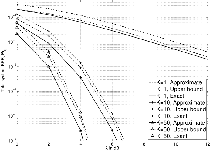
Figure 1: Total system BERs ${\rm Pr}_{b,e}(K)$, ${\rm Pr}_{b,u}(K)$ and ${\rm Pr}_{b,a}(K)$ for $K$-GA when $K=\bar{K}=1,10,50$.

Fig. 1 illustrates the exact, UB, and approximate BER’s, i.e., (17), (18), and (19), of the $K$-GA scheme for $\bar{K}=K=1,10,50$. It can be seen from this figure that the UB and approximate expressions produce the BER curves which lay within 0.5 dB of the exact BER.

IV Optimal selection of the number of active users

Two scenarios are considered in this section for selecting the number of active users $K$ optimally: (i) minimizing ${\rm Pr}_{b}^{K-GA}(\cdot)$ while $E_{T}^{K-GA}$ remains constant and (ii) minimizing $E_{T}^{K-GA}$ while ${\rm Pr}_{b}^{K-GA}(\cdot)$ is constrained to be acceptably small. Optimization problems for each scenario are provided.

The set of candidate values of $K$ is the set of all positive integers smaller than or equal to $\bar{K}$, i.e, ${\cal K}\triangleq\{1,\cdots,\bar{K}\}$. Note that due to hardware design limitations ${\cal K}$ can be just a set of some integers smaller than or equal to $\bar{K}$. The latter case can be easily adopted in the methods developed further.

IV-A Optimal selection of $K$ based on system BER minimization

Using (2) and (10), under the finite energy constraint, we can find that the achievable energy gain for $E_{d}(K)$ determines $\lambda(K)$ in ${\rm Pr}_{b}^{K-GA}(\cdot)$ as follows

$$\lambda(K)=E_{d}(K)~{}c/(NT_{s})=\left((\bar{K}-K)\alpha^{-1}+1\right)E_{d}^{GA}~{}c/(NT_{s})$$ (20)

where $c=\bar{K}(\sum_{k=1}^{\bar{K}}\sigma_{k}^{-2})^{-1}/\omega$. It is worth mentioning that $E_{d}^{GA}/(NT_{s})$ in (20) stands for the average transmit power over $N$ slots when $K=\bar{K}$. Thus, it can be denoted as $\lambda^{GA}$. Using this notation, (20) can be represented as

$$\lambda(K)=\left((\bar{K}-K)\alpha^{-1}+1\right)~{}c~{}\lambda^{GA}.$$ (21)

It can be seen from (21) that a power gain of $\left((\bar{K}-K)\alpha^{-1}+1\right)c$ in ${\rm Pr}_{b}^{K-GA}(\cdot)$ is achieved if $K<\bar{K}$. Denoting $P_{T}=E/(NT_{s})$ as the total average power consumed by all users during one slot, $\lambda(K)$ can be also expressed in terms of $P_{T}$ as $\lambda(K)=c(P_{T}-K\alpha^{-1}\lambda^{GA})$.

Using $\lambda(K)$ in (21), we optimize $K$ for a given $\omega$ to minimize the system BER while satisfying the finite energy constraint. The corresponding optimization problem can be mathematically formulated as

$$K_{b}^{*}=\arg\min_{K\in{\cal K}}{\rm Pr}_{b}^{K-GA}(K)\hskip 14.22636pt\text{subject to}\hskip 14.22636ptE_{T}^{K-GA}=E.$$ (22)

One way to solve (22) is to employ a binary search over $K\in{\cal K}$ through direct computation of ${\rm Pr}_{b}^{K-GA}(\cdot)$. However, direct evaluation of ${\rm Pr}_{b}^{K-GA}(\cdot)$ is computationally complex, and such an approach can be inaccessible for applications sensitive to high computational complexity. Therefore, an approach, which avoids direct computation of ${\rm Pr}_{b}^{K-GA}(\cdot)$ for all $K$, is proposed.

To this end, let us relax $K$ to be a real number such that $K\in[1,\bar{K}]$. Let us also define $\eta(\cdot)\triangleq\frac{\partial}{\partial K}{\rm Pr}_{b}^{K-GA}(\cdot)$. It can be observed that ${\rm Pr}_{b}^{K-GA}(\cdot)$ is convex with respect to $K$ due to the fact that $\frac{\partial^{2}}{\partial^{2}K}{\rm Pr}_{b}^{K-GA}(\cdot)\geq 0$. Thus, the minimum of ${\rm Pr}_{b}^{K-GA}(\cdot)$ over $K\in[1,\bar{K}]$ can be found by minimizing $\big{|}\eta(\cdot)\big{|}$ for a given normalized $\Omega$, i.e., $\Omega_{N}=\omega\lambda^{GA}$. Note that this minimum is unique. Therefore, denoting $K^{*}$ as a real-valued solution, the corresponding optimal solution can be given by

$$K^{*}=\arg\min_{K\in[K_{n},K_{1}]}\Big{|}\eta(K)\Big{|}.$$ (23)

Recall that ${\cal K}$ is a finite set of integers, and the optimal $K^{*}_{b}\in{\cal K}$ may not be equivalent to $K^{*}$ in (23). Therefore, (23) should be reformulated as

$$K^{*}_{b}=\begin{cases}\bar{K},&\text{if}\hskip 2.84544pt\text{sign}(\eta(K=\bar{K}))=-1\\ 1,&\text{else if}\hskip 2.84544pt\text{sign}(\eta(K=1))=1\\ \arg\min_{K\in\{K_{i},K_{i+1}\}}{\rm Pr}_{b}^{K-GA}(K),&\text{otherwise}\end{cases}$$ (24)

where ${\rm sign}(a)=|a|/a$ for $a\in\mathbb{R}$ with ${\rm sign}(0)=1$, and $K_{i}\in{\cal K}$ is the largest integer smaller than $K^{*}$ that satisfies the equality ${\rm sign}(\eta(K_{i})){\rm sign}(\eta(K_{i+1}))=-1$.

In order to find $K^{*}_{b}\in{\cal K}$, we first compute ${\rm sign}(\eta(K))$ at $K=\bar{K}$ (and/or $K=1$). If the resulting ${\rm sign}(\cdot)$ is $-1$ (or $1$), then we select $K^{*}_{b}=\bar{K}~{}(\text{or }1).$ Otherwise, $K_{i}\in{\cal K}$ can be found by binary search algorithm followed by selecting $K^{*}_{b}$ at whichever of $K_{i}$ or $K_{i+1}$ that has a smaller ${\rm Pr}_{b}^{K-GA}(\cdot)$.

Considering, for example, the case when ${\rm Pr}_{b}^{K-GA}(\cdot)={\rm Pr}_{b,a}^{K-GA}(K)$, it is shown in Appendix that

$$\eta(K)=\frac{1}{K}-\sum_{l=0}^{f(K)}\frac{1}{K+l}-f^{\prime}(K)\sum_{l=0}^{K-1}\frac{1}{1+f(K)+l}$$ (25)

where $f(K)\triangleq g_{a}\omega\lambda$.

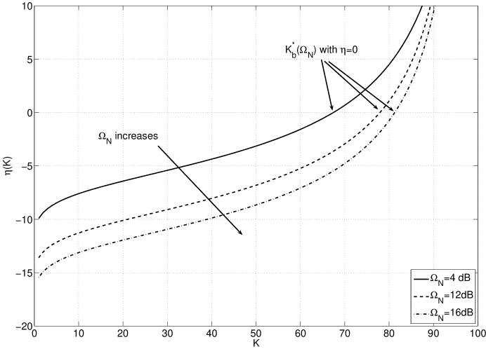
Figure 2: Function $\eta(\cdot)$ versus $K$ when $\bar{K}=100,$ $M=4,$ and $\alpha=1.$

Given $\Omega_{N}$ and a finite set ${\cal K}=\{1,2,\cdots,\bar{K}\},$ $\eta(K)$ is illustrated in Fig. 2. It is shown that neither $K\rightarrow 1$ nor $K\rightarrow\bar{K}$ may minimize ${\rm Pr}_{b}^{K-GA}(\cdot)$. Therefore, for a given $\Omega_{N}$, there exists an optimal $1\leq K^{*}_{b}\leq\bar{K}$ minimizing ${\rm Pr}_{b}^{K-GA}(\cdot)$. For example, it can be seen from the figure that when $M=4$ and $\bar{K}=100$, $K^{*}_{b}\approx 67$ minimizes ${\rm Pr}_{b}^{K-GA}(\cdot)$ at $\Omega_{N}=4$ dB.

IV-B Optimal selection of $K$ based on $E_{T}^{K-GA}$ minimization

If an MU system is capable of recovering properly the transmitted information as long as the system BER is less than or equal to a predefined desired level, the optimal $K$ can be found via minimization of $E_{T}^{K-GA}$ in (7) subject to the constraint ${\rm Pr}_{b}^{K-GA}(\cdot)\leq{\rm BER}_{t}$ where ${\rm BER}_{t}$ is the required target BER. In this problem, different from the previous problem, $E_{T}^{K-GA}$ is the optimization variable, while $\lambda$ (equivalently $\Omega_{N}=\Omega$) is fixed.

Two cases of delay tolerant and delay sensitive systems are of interest.

IV-B1 Delay tolerant (DT) systems

The constrained optimization problem for finding optimal $K$ can be written in this case as

$$K_{dt}^{*}={\rm arg}\min_{K\in{\cal K}}E_{T}^{K-GA}\hskip 14.22636pt\text{subject to}\hskip 14.22636pt{\rm Pr}_{b}^{K-GA}(K)\leq{\rm BER}_{t}.$$ (26)

Note that for a given $\Omega$, ${\rm Pr}_{b}^{K-GA}(\cdot)$ and $E_{T}^{K-GA}$ are, respectively, monotonically decreasing and monotonically increasing functions of $K$. Thus, among all values of $K$ satisfying the constraint ${\rm Pr}_{b}^{K-GA}(\cdot)\leq{\rm BER}_{t}$, the smallest $K\in{\cal K}$ which minimizes $E_{T}^{K-GA}$ is the solution of (26).

In order to find $K_{dt}^{*}\in{\cal K}$, we first need to find ${\rm Pr}_{b}^{K-GA}(\cdot)$ when $K=\bar{K}.$ If $\bar{K}$ does not satisfy the system BER requirements, then $K^{*}_{dt}=0$. When $K^{*}_{dt}=0$, the system may allow delays to prevent the waste of the total energy of all users. Otherwise, the smallest $K\leq\bar{K}$, which satisfies the system BER requirements, can be searched efficiently using, for example, a binary search algorithm.

IV-B2 Delay sensitive (DS) systems

DS systems allow to transmit data even if ${\rm Pr}_{b}^{K-GA}(\cdot)~{}>~{}{\rm BER}_{t}$ when $K=\bar{K}.$ Then, the corresponding constrained optimization problem can be written as

$$K_{ds}^{*}=\begin{cases}\arg\min_{K\in{\cal K}}\hskip 2.84544ptE_{T}^{K-GA}\;\text{subject to}\;{\rm Pr}_{b}^{K-GA}(K)\leq{\rm BER}_{t},&{\rm if}\;{\rm Pr}_{b}^{K-GA}(\bar{K})\!\leq\!{\rm BER}_{t}\\ K_{1},&{\rm otherwise}.\end{cases}$$ (27)

The problem (27) can be solved similar to the previous one. The only difference is that $K^{*}_{ds}=\bar{K}$ even if $K=\bar{K}$ is not sufficient to satisfy the constraint ${\rm Pr}_{b}^{K-GA}(\cdot)\leq{\rm BER}_{t}$.

V Asymptotic analysis

V-A Asymptotic analysis of optimal $K$ based on $E_{T}^{K-GA}$ minimization

In general, the optimum $K$ based on $E_{T}^{K-GA}$ minimization under fixed system BER cannot be found in closed form. However, its asymptotic behavior can be studied analytically. Recall that the derived system BER expressions depend on the beta function ${\rm B}(\cdot,\cdot)$. Thus, we first study the asymptotic behavior of ${\rm B}(\cdot,\cdot)$ with respect to $K$.

The following theorem summarizes the asymptotic behavior of the beta function.

Theorem 1

Let $x$ and $y$ be two positive integers. When $x\rightarrow\infty$, we have

$$\lim_{x\rightarrow\infty}x^{y}\hskip 2.84544pt{\rm B}(x,y)=\Gamma(y)$$ (28)

where $\Gamma(y)=\int_{0}^{\infty}t^{y-1}{\rm e}^{-t}{\rm d}t$ denotes the complete gamma function.

Proof: The beta function can be alternatively represented in terms of the following ratio of complete gamma functions

$${\rm B}(x,y)=\frac{\Gamma(x)\Gamma(y)}{\Gamma(x+y)}.$$ (29)

Using the expression $\Gamma(x)=(x-1)!$ for the gamma function, we can find the following ratio

$$\frac{\Gamma(x)}{\Gamma(x+y)}=\frac{(x-1)!}{(x+y-1)!}=\frac{1}{(x+y-1)(x+y-2)\cdots(x+1)x}.$$ (30)

Since $(x+y-1)(x+y-2)\cdots(x+1)x$ in (30) is dominated by the first power term $x^{y}$, the ratio in (30), for $x\rightarrow\infty$, becomes

$$\lim_{x\rightarrow\infty}\Gamma(x)/\Gamma(x+y)=x^{-y}.$$ (31)

Thus, when $x\rightarrow\infty$, inserting (31) into (29) reveals the asymptotic behavior of (29) as

$$\lim_{x\rightarrow\infty}\hskip 2.84544pt{\rm B}(x,y)=\lim_{x\rightarrow\infty}\frac{\Gamma(x)}{\Gamma(x+y)}\Gamma(y)=x^{-y}\hskip 2.84544pt\Gamma(y).$$ (32)

Since for a given $y$, $\Gamma(y)$ in (32) is fixed, (28) is obtained when $x\rightarrow\infty$. $\blacksquare$

Theorem 1 enables us to evaluate the system BER for two asymptotic cases of (i) large $K$ and (ii) high SNR. We also aim at investigating how the optimal $K$ scales asymptotically. For simplicity, only the approximate BER expression (19) is considered in the further analysis.

For the case of large $K$, we aim at analyzing ${\rm Pr}_{b,a}^{K-GA}(K)$ versus $K$ and SNR. As per Theorem 1, for large values of $x$, the following approximation holds true ${\rm B}(x,y)\approx x^{-y}\Gamma(y)$. Then, when interpreting $x$ and $y$ in (28) as $K$ and $1+g_{a}\Omega$, respectively, the system BER can be expressed for large values of $K$ as

$$\begin{split}{\rm Pr}_{b,a}^{K-GA}(K)&=K^{-g_{a}\Omega}0.2\hskip 2.84544pt\Gamma(1+g_{a}\Omega)\\ \quad&=\Theta\left(K^{-{\rm SNR}}\right)\end{split}$$ (33)

where we use the alternative notation SNR$=\Omega$ in the last expression. Therefore, (33) shows how the system BER scales with respect to the MUDiv gain if $K$ is large.

For another asymptotic case of large SNR, ${\rm Pr}_{b,a}^{K-GA}(K)$ can also be expressed in terms of SNR and $K$. Specifically, using the fact that ${\rm B}(x,y)={\rm B}(y,x),$ it follows straightforwardly from Theorem 1 that for large $y$, ${\rm B}(x,y)\approx y^{-x}\Gamma(x).$ Therefore, the system BER ${\rm Pr}_{b,a}^{K-GA}(K)$ can be expressed for large SNR as

$$\begin{split}{\rm Pr}_{b,a}^{K-GA}(K)&=\Omega^{-K}0.2\hskip 2.84544ptg_{a}^{-K}\Gamma(K+1)\hskip 2.84544pt\\ \quad&=\Theta\left({\rm SNR}^{-K}\right).\end{split}$$ (34)

It follows from (34) that the total system BER scales inversely with the order of the SNR, i.e, the MUDiv is equal to $K$.

Using (33) and (34), we can find the optimal $K^{*}\in{\cal K}$, i.e., either $K^{*}_{dt}$ for the delay tolerant or $K^{*}_{ds}$ for the delay sensitive systems.

In the case when $K$ is large, it can be found using (33) that for given $\omega$, $\lambda$, and ${\rm BER}_{t}$, the optimal $K^{*}\in{\cal K}$, i.e., $K^{*}_{dt}$ for the delay tolerant or $K^{*}_{ds}$ for the delay sensitive systems, must satisfy the following inequality

$$\begin{split}K^{*}&\geq\left(0.2\Gamma(1+g_{a}\Omega)\right)^{\frac{1}{g_{a}\Omega}}{\rm BER}_{t}^{-\frac{1}{g_{a}\Omega}}\\ \quad&=\Theta\left({\rm BER}_{t}^{-1/{\rm SNR}}\right).\end{split}$$ (35)

It follows from (35) that for large $K$ and a given SNR, $K^{*}$ is an exponentially decreasing function of ${\rm BER}_{t}$.

In the case of high SNR, it can be found from (34) that the optimal $K^{*}$, which guarantees that the target BER is archived, i.e., the constraint ${\rm Pr}_{b,a}^{K-GA}(K)\leq{\rm BER}_{t}$ is satisfied, must obey the following inequality

$$K^{*}\geq\frac{\log{\rm BER}_{t}^{-1}}{\log g_{a}\Omega}=\Theta\left(\frac{\log{\rm BER}_{t}^{-1}}{\log{\rm SNR}}\right).$$ (36)

For a given ${\rm BER}_{t}$, it follows from (36) that the corresponding optimal $K^{*}$, i.e., $K^{*}_{dt}$ for the delay tolerant or $K^{*}_{ds}$ for the delay sensitive systems, is proportional to the inverse of $\log{\rm SNR}$. Moreover, unlike the case of large $K$, in the case of high SNR, $K^{*}$ decreases in a log-scale with ${\rm BER}_{t}$.

V-B Asymptotic analysis of optimal $K$ based on the system BER minimization

We again consider two cases of (i) large $K$ and (ii) high SNR and study the asymptotic behavior of optimal $K^{*}_{b}$, i.e., we study the asymptotic behavior of the solution of the optimization problem (34). For simplicity, but without any loss of generality, we assume that $c=1$.

In the case when $K$ is large, we first determine how the system BER scales with $K$ while satisfying the finite energy constraint. The corresponding power gain given by (21) is $G_{p}\triangleq\left((\bar{K}-K)\alpha^{-1}+1\right).$ Using this notation and (33), the system BER can be asymptotically expressed as

$$\begin{split}{\rm Pr}_{b,a}^{K-GA}(K)&=0.2\Gamma(1+g_{a}G_{p}\Omega_{N})K^{-g_{a}G_{p}\Omega_{N}}\\ \quad&=\Theta\left({K}^{-G_{p}{\rm SNR}}\right)\end{split}$$ (37)

where we use the alternative notation SNR$=\Omega_{N}$. Therefore, if $K\gg\bar{K}-K$, the achievable MUDiv gain is determined by $G_{p}(K)\cdot{\rm SNR}=\left((\bar{K}-K)\alpha^{-1}+1\right)\cdot{\rm SNR}$ instead of ${\rm SNR}$. It is also worth mentioning that, for a given SNR, the asymptotic system BER scales exponentially with $K^{(\bar{K}-K)/\alpha}$. The latter means, in particular, that the achievable system BER is lower in the case of using optimal $K$ as compared to the case when all users are active, i.e., $K=\bar{K}$.

In the case of high SNR, using $G_{p}$ and (34), the asymptotic expression for the system BER can be obtained as

$$\begin{split}{\rm Pr}_{b,a}^{K-GA}(K)&=0.2g_{a}^{-K}\Gamma(K+1)(G_{p}\Omega_{N})^{-K}\\ \quad&=\Theta\left((G_{p}{\rm SNR})^{-K}\right).\end{split}$$ (38)

It follows from (38) that the asymptotic system BER benefits from the MUDiv power gain $G_{p}^{-K}=\left((\bar{K}-K)\alpha^{-1}+1\right)^{-K}$ at the cost of having the diversity order $K<{\bar{K}}$.

Finally, inserting (38) into (23), we obtain that

$$\begin{split}\lim_{SNR\rightarrow\infty}K^{*}_{b}&=\arg\min_{K}\left|\frac{\partial}{\partial K}(\ref{eq:asymp_Prb4})\right|=\arg\min_{K}\left|G_{p}\cdot{\rm SNR}\right|\\ \quad&=\bar{K}+\alpha\end{split}$$ (39)

where $0\leq\alpha\leq 1$. Since optimal MUDiv $K$ is restricted to be integer, it can be concluded from (39) that the MUDiv $K=\bar{K}$ is optimal when SNR$\rightarrow\infty$. The latter means that the maximum available MUDiv should be used for energy unlimited systems that agrees with known results.

VI Extension to multiple antenna MU systems

The optimization problems proposed in Section IV can be extended to multiple antenna MU systems, which will also allow to use the benefits of multiple antenna techniques [19, 20]. Toward this end, a generalized expression for the average BER has to be derived. For brevity, we consider only the approximate average system BER case.

Let $D$ denote the multiple antenna diversity order. Then, in the multiple antenna case, the degrees of freedom (DOF) of $y$ in (14) extends to $2D$, that is, $y\sim\chi_{2D}^{2}$ where $\chi^{2}_{2D}$ stands for the Chi-squared distribution with $2D$ DOF (refer also to [20]). Therefore, for given $K$ and $D$, the expression for $p_{\rho}^{K-GA}(y)$ in (15) can be generalized as [19]

$$p_{\rho}^{K-GA}(y)=K\frac{{\rm e}^{-y/\Omega}}{\Omega}\gamma\left(D,y/\Omega\right)^{K-1}\frac{\left(y/\Omega\right)^{D-1}}{\Gamma(D)^{K}}$$ (40)

where $\gamma(a,b)\triangleq\int_{0}^{b}t^{a-1}{\rm e}^{-t}{\rm d}t$ denotes the lower incomplete gamma function [18].

Inserting (40) into (14), we obtain the average BER in the multiple antenna case as

$${\rm Pr}^{K-GA}_{b}(K)=0.2K\int_{0}^{\infty}t^{D-1}{\rm e}^{-(1+g_{a}\Omega)t}\gamma(D,t)^{K-1}/\Gamma(D)^{K}\hskip 2.84544pt{\rm d}t.$$ (41)

Finally, the optimization problems proposed Section IV can be straightforwardly extended to the case of multiple antenna MU systems by using (41) instead of the corresponding BER expressions for the single antenna case. As an example, an extension of the problem (22) to the case of multiple antenna MU systems will be investigated numerically in the following section.

VII Numerical results

Consider an MU system with Gray-coded square M-QAM of size $M\in\{4,64\}$. Let $(C_{M,1},c_{M,1})$ in (13) be ($1,1$) for $M=4$, while $\{(C_{M,1},c_{M,1}),\cdots,$ $(C_{M,5},c_{M,5})\}$ be $\{(7/12,1/21),(1/2,3/7),$
$(-1/12,25/21),(1/12,9^{2}/21),(-1/12,13^{2}/21)\}$ for $M=64$ [16]. Independent log–normal distributed shadowing with mean $\mu=1$ and standard deviation $\nu=5$ is assumed with pathloss 0 dB. Considering the approximate BER, i.e., ${\rm Pr}_{b}^{K-GA}(\cdot)={\rm Pr}_{b,a}^{K-GA}(K)$, the optimal $K$, i.e., $K^{*}_{b}$ of (24), $K^{*}_{dt}$ of (26), or $K^{*}_{ds}$ of (27), are found. The set ${\cal K}=\{1,2,\cdots,\bar{K}\}$, $c=1$, $\alpha\in\{1,2,7.81,31.25\},$ and $E_{d}(K)/E_{f}\in[\alpha,\bar{K}-1+\alpha]$ are used. Note that the parameter $\alpha=2$ corresponds to the standard case when $280$ pilot sub-carriers and $560$ data sub-carriers are used per one sub-channel in $10$ MHz uplink WiMAX (IEEE 802.16e) [21]. For comparisons, we also consider other parameter values. For example, the parameter $\alpha=7.81$ can be obtained by using 32 pilot and 250 data sub-carriers while $\alpha=31.25$ results from using 32 pilot and 1000 data sub-carriers.

In the case when $\bar{K}=100$ and $\alpha=1$, the ratio $\lambda(K)/\lambda^{GA}$ (or, equivalently, $E_{d}(K)/E_{d}^{GA}$) is set at the values between 0 dB and 20 dB depending on $K$. The generic GA scheme is also depicted for comparison.

VII-A Minimizing the system BER

Example 1: In our first example, we consider the problem (24) and the case when for a given $\Omega_{N}\in\{5,10\}$ dB and $\alpha=2$, total energy grows with $\bar{K}$. Note that $E_{T}^{K-GA}$ (or, equivalently, the average power $P_{T}(K)$) is an increasing function of $\bar{K}$.

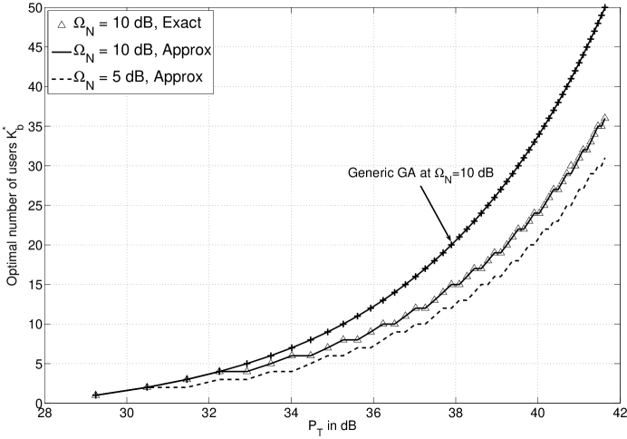
Figure 3: Optimal number of users $K^{*}_{b}$ versus $P_{T}$ for different $\Omega_{N}$, $M=4,$ and $\alpha=2.$

Fig. 3 shows $K^{*}_{b}$ of (24) versus $P_{T}$ for various values of $\Omega_{N}$. It can be seen from the figure that $K^{*}_{b}$ increases with respect to $P_{T}$. The latter means that the maximum available MUDiv should be used for energy unlimited systems, while the optimal MUDiv can be significantly smaller than the maximum available MUDiv $\bar{K}$ for energy limited systems. It can also be observed that for a given $P_{T}$ and low $\Omega_{N}$, the optimal MUDiv $K^{*}_{b}$ is also small and more energy should be allocated for actual data transmission $E_{d}(K)$ in order to achieve better BER. Finally, it can be also seen in this figure that $K^{*}_{b}$ of (24) that minimizes the approximate BER coincides with $K^{*}_{b}$ of (24) that minimizes the exact BER, which validates the use of approximate BER.

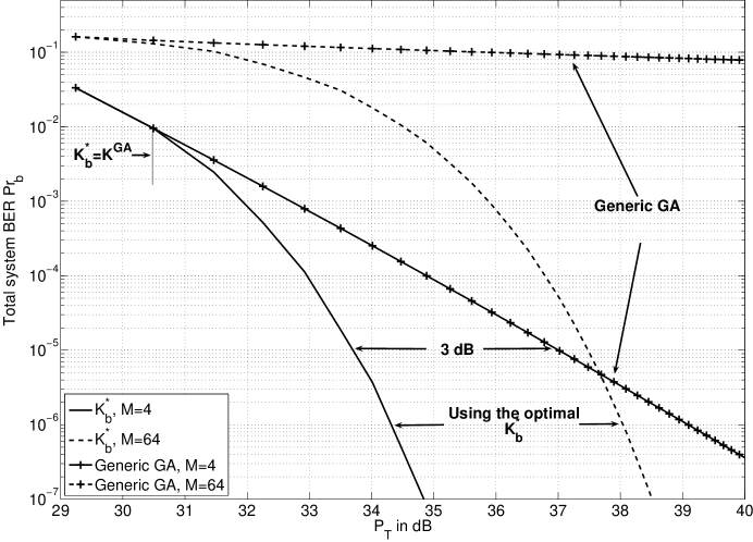
Figure 4: Total system BER using $K^{*}_{b}$ versus $P_{T}$ when $\Omega_{N}=5$ dB, $M=4,64,$ and $\alpha=2.$

Fig. 4 illustrates the impact of $K^{*}_{b}$ on ${\rm Pr}_{b}^{K-GA}(\cdot)$ versus $P_{T}$. In this figure, $\Omega_{N}=5$ dB and $\alpha=2$ are taken. It can be seen from the figure that ${\rm Pr}_{b}^{K-GA}(\cdot)$ based on $K^{*}_{b}$ is a decreasing function of $P_{T}$. Moreover, for $M=4$ and $P_{T}\leq 30.5$ dB, the generic GA scheme is optimal since it provides minimum ${\rm Pr}_{b}^{K-GA}(\cdot)$ and $K^{*}_{b}=\bar{K}$, in this case. However, when $P_{T}\geq 30.5$ dB, the optimal $K^{*}_{b}<\bar{K}$ is obtained. For example, when $M=4$, $K^{*}_{b}$ provides 3 dB power gain at ${\rm Pr}_{b}=10^{-5}$ as compared to the generic GA.

Example 2: In the second example, we consider the problem (24) and the case when for a given maximum achievable MUDiv $\bar{K}$, $E_{T}^{K-GA}$ grows with $\Omega_{N}$. In this case, $\alpha\in\{7.8125,31.25\}$ and $\bar{K}=50$ are used.

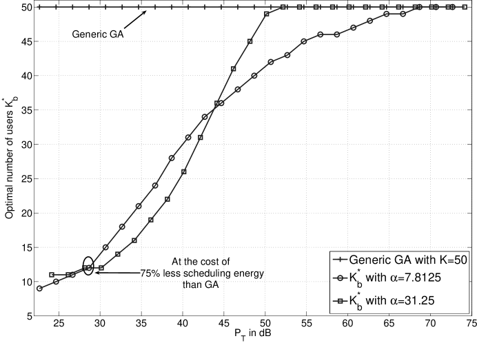
Figure 5: Optimal number of users $K^{*}_{b}$ versus $P_{T}$ when $\bar{K}=50,$ $M=4,$ $\alpha\in\{7.8125,31.25\}.$

Fig. 5 shows $K^{*}_{b}$ versus $P_{T}$. It can be seen from the figure that $K^{*}_{b}$ is an increasing function of $P_{T}$ and it converges to $\bar{K}$ if more power (energy) is available for all users in the system. The convergence rate depends on $\alpha$ and it is higher for larger $\alpha$ and slower for smaller $\alpha$. Note that the practical values of $\alpha$ are smaller than both values tested in this example (see Example 1). It can also be observed that for low $P_{T}$, less $K^{*}_{b}E_{f}$ is required to achieve a better system BER than the one achieved if all $\bar{K}$ users are active. For example, for $P_{T}=28$ dB and $\alpha=7.8125$, the achieved $K^{*}_{b}E_{f}$ for $K^{*}_{b}=12$ is significantly smaller than the one for the generic GA.

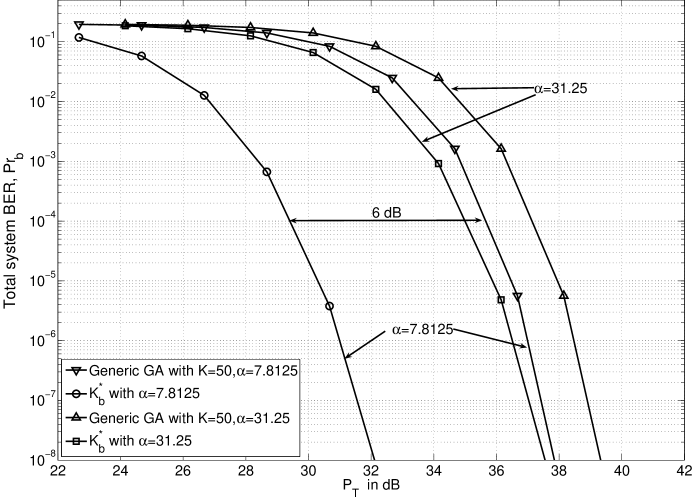
Figure 6: Total system BER using $K^{*}_{b}$ versus $P_{T}$ when $\bar{K}=50,$ $M=4,$ $\alpha\in\{7.8125,31.25\}.$

In Fig. 6, the impact of $K^{*}_{b}$ on ${\rm Pr}_{b}^{K-GA}(\cdot)$ is illustrated versus $P_{T}$. A significant power gain is provided by the proposed method as compared to the generic GA scheme. For example, in the case when $\alpha=7.8125,$ the use of $K^{*}_{b}$ provides $6$ dB power gain at ${\rm Pr}_{b}^{K-GA}(\cdot)=10^{-4}$. A significant power gain can be observed even for large $\alpha$, i.e., $\alpha=31.25$. However, regardless of $\alpha$, the aforementioned power gain vanishes and $K^{*}_{b}$ converges to $\bar{K}$ if $P_{T}\rightarrow\infty$ (see also Fig. 5).

VII-B Minimizing the total energy of all users in the system

Example 3: In the last example, we consider the problems (26) and (27) for the DT and DS MU systems, correspondingly. The proposed $K$-GA scheduling scheme based on $K^{*}_{dt}$ of (26) and $K^{*}_{ds}$ of (27) is compared to the generic GA scheduling scheme.

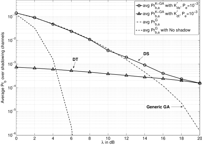
Figure 7: Average ${\rm Pr}_{b}$ of $K$-GA in DS MU and DT MU systems when $\mu=1,$ $\nu=5,$ ${\rm BER}_{t}=10^{-3},$ $\alpha=1,$ $\bar{K}=100.$

Fig. 7 shows the error probability of the proposed $K$-GA scheduling scheme ${\rm Pr}_{b}^{K-GA}(\cdot)$ averaged over variations of the channel mean $\omega$ versus $\lambda$. The parameters $\bar{K}=100$ and ${\rm BER}_{t}=10^{-3}$ are taken. The average error probability of the generic GA is computed for two cases with and without variations of the channel mean $\omega$. In can be seen from the figure that the average ${\rm Pr}_{b}^{K-GA}(\cdot)$ is maintained below the system requirements (i.e., ${\rm BER}_{t}=10^{-3}$) for the DT MU system. For the DS MU system, the average ${\rm Pr}_{b}^{K-GA}(\cdot)$ is close to the average ${\rm Pr}_{b,a}^{GA}(\cdot)$ at low SNRs since in order to guarantee a given target BER ${\rm BER}_{t}$, the outage is not allowed even if $\bar{K}$ is not sufficiently large. It can be also seen that as $\lambda$ increases, the DS MU system performs closer to the DT MU system. It is because $K\leq\bar{K}$ is sufficiently large to guarantee the target ${\rm BER}_{t}$ in both cases.

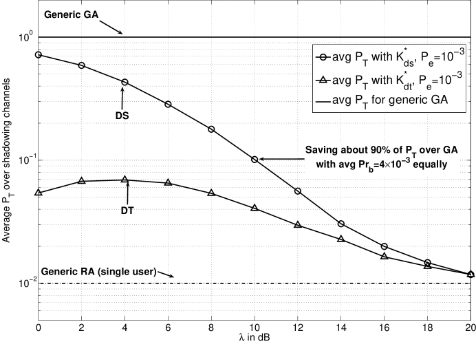
Figure 8: Average $P_{T}$ of $K$-GA in DS MU and DT MU systems when $\mu=1,$ $\nu=5,$ $\bar{K}=100,$ $\alpha=1,$ ${\rm BER}_{t}=10^{-3}.$

Based on $K^{*}_{dt}$ and $K^{*}_{ds}$, it can also be seen in Fig. 8 that the average $P_{T}$ normalized by the power required for the generic GA is a decreasing function of $\lambda$ for both the DT and DS MU systems. Moreover, the DT MU system requires less power (energy) than the DS MU system while satisfying the system requirement on target BER ${\rm BER}_{t}$. For example, at $\lambda\approx 10$ dB, the DS MU systems with ${\rm BER}_{t}=10^{-3}$ achieves a power saving gain of $10$ dB over the generic GA for the same average ${\rm Pr}_{b}=4\times 10^{-3}$ (see Figs. 7 and 8). Figs. 7 and 8 also depict that as $\lambda$ increases, $P_{T}$ converges to the power required for the RA scheduling scheme.

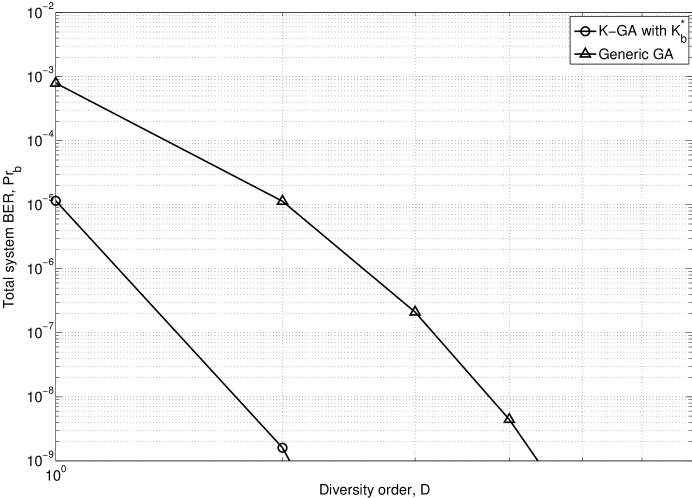
Figure 9: Impacts of $D,$ i.e., $2D$ is the DOF resulting from multiple antennas, on ${\rm Pr}_{b}^{K-GA}$ using $K^{*}_{b}$ when ${\bar{K}}=5,$ $\Omega_{N}=5$ dB, and $M=4.$

For the multiple antenna case, Fig. 9 shows ${\rm Pr}_{b}^{K-GA}(\cdot)$ versus the diversity order $D$ for the following parameters $\bar{K}=5$, $\Omega_{N}=5$ dB, $\alpha=1,$ and $M=4$. It is also assumed that the energy is distributed according to (22) with ${\rm Pr}^{K-GA}_{b}(\cdot)$ as derived in Section VI. It can be seen from this figure that our optimal energy distribution gives a boost in the system BER as compared to the generic GA scheduling scheme.

VIII Conclusions

A new realistic energy model which describes the distribution of the total finite users’ energy between scheduling and data transmission stages is developed for the energy limited uplink MU wireless systems. MU scheduling algorithms which maximize the MUDiv gain are derived for the aforementioned systems to (i) minimize the overall system BER for a fixed total energy of all users in the system or (ii) minimize the total energy of all users for fixed BER requirements. It is shown that for a fixed number of available users, an achievable MUDiv gain can be improved by activating only a subset of users from the entire set of users. Using asymptotic analysis, it is shown that our approach benefits from MUDiv gains higher than that achieved by the generic GA algorithm, which is the optimal scheduling method for energy unlimited systems. In particular, when minimizing the system BER, it is found that the achieved MUDiv gain is determined by $\left((\bar{K}-K)\alpha^{-1}+1\right)\cdot{\rm SNR}$ when $K$ is large. Moreover, in the case of high SNR, the MUDiv power gain $\left((\bar{K}-K)\alpha^{-1}+1\right)^{-K}$ can be archived while obtaining the diversity order $K$. Simulation results validate our theoretical observations and show that the proposed $K$-GA algorithm based on optimizing the number of active users provides significant energy gains for energy limited MU wireless systems over the generic GA algorithm.

Appendix: Derivations of (23) and (25)

Using (19), the first derivative of ${\rm Pr}_{b,a}^{K-GA}(K)$ in the optimization problem (24) can be expressed as

$$\frac{\partial}{\partial K}{\rm Pr}_{b,a}^{K-GA}\left(K\right)=b{\rm B}(K,1+f(K))+bK\frac{\partial}{\partial K}{\rm B}\left(K,1+f(K)\right).$$ (42)

In turn, the first derivative of ${\rm B}\left(K,1+f(K)\right)$ with respect to $K$ in (42) can be written as

$$\frac{\partial}{\partial{K}}{\rm B}\left(K,1+f(K)\right)=\frac{\partial}{\partial{K}}\int_{0}^{1}t^{K-1}(1-t)^{f(K)}{\rm d}t=\int_{0}^{1}\frac{\partial}{\partial{K}}\hskip 2.84544ptt^{K-1}(1-t)^{f(K)}{\rm d}t.$$ (43)

or equivalently as

$$\frac{\partial}{\partial K}{\rm B}(K,1+f(K))=\int_{0}^{1}\left(1-t\right)^{f(K)}t^{K-1}\hskip 2.84544pt{\rm ln}t\hskip 2.84544pt{\mathrm{d}}t+f^{\prime}(K)\int_{0}^{1}\left(1-t\right)^{K-1}t^{f(K)}\hskip 2.84544pt{\rm ln}\hskip 1.42271ptt\hskip 2.84544pt{\mathrm{d}}t$$ (44)

where $f^{\prime}(\cdot)$ denotes the first derivative of $f(\cdot)$ with respect to $K$ and ${\rm ln}(\cdot)$ stands for the natural logarithm.

Using the relationship [18, (4.253.1)]

$$\int_{0}^{1}x^{u-1}(1-x^{r})^{v-1}{\rm ln}\hskip 1.42271ptx\hskip 2.84544pt{\rm d}x={\rm B}\left(u/r,v\right)\big{\{}\psi(u/r)-\psi(u/r+v)\big{\}}/r^{2}$$ (45)

where $\psi(z)=\frac{\partial}{\partial z}{\rm ln}\Gamma(z)$ denotes the digamma function for $z>0$, the first derivative of the beta function in (44) can be written as

$$\begin{split}\frac{\partial}{\partial K}{\rm B}(K,1+f(K))&={\rm B}(K,1+f(K))\\ \quad&\times\big{\{}\psi(K)-(1+f^{\prime}(K))\psi(K+1+f(K))+f^{\prime}(K)\psi(1+f(K))\big{\}}.\end{split}$$ (46)

Inserting (46) into (42), we find that the solution of (24) should satisfy the following equation

$${\rm B}(K,1+f(K))\Big{[}1+K\big{\{}\psi(K)-(1+f^{\prime}(K))\psi(K+1+f(K))+f^{\prime}(K)\psi(1+f(K))\big{\}}\Big{]}=0.$$ (47)

Since in our system model $K\geq 1$ and $f(K)\geq 0$, it follows from (47) that ${\rm B}(K,1+f(K))\geq 0$. Therefore, the equality ${\rm B}(K,1+f(K))=0$ holds if and only if $K$ goes to infinity. However, for $K\rightarrow\infty$ the assumption of the limited total system user energy is violated, and therefore, ${\rm B}(K,1+f(K))$ in (47) must always be positive. Thus, the problem of finding the solution of (24) boils down to the problem of finding the number of users which satisfies the following equation

$$\psi(K)-\psi(K+1+f(K))+f^{\prime}(K)\big{\{}\psi(1+f(K))-\psi(K+1+f(K))\big{\}}+1/K=0.$$ (48)

Using the following expression [18, (8.365.3)]

$$\psi(x+n)=\psi(x)+\sum_{l=0}^{n-1}(x+l)^{-1}$$ (49)

the differences between the digamma functions in (48) can be represented alternatively as

$$\psi(K+1+f(K))-\psi(1+f(K)) =\sum_{l=0}^{K-1}\left(1+f(K)+l\right)^{-1}.$$ (50)

$$\psi(K+1+f(K))-\psi(K) =\sum_{l=0}^{f(K)}\left(K+l\right)^{-1}.$$ (51)

Finally, inserting (50) and (51) into (48), the left hand side of (48) can be rewritten as

$$\eta(K)=\frac{1}{K}-\sum_{l=0}^{f(K)}\frac{1}{K+l}-f^{\prime}(K)\sum_{l=0}^{K-1}\frac{1}{1+f(K)+l}.$$ (52)

Therefore, for given $\Omega$ and $E_{T}^{K-GA}$, the optimization problem (22) can be rewritten as

$$K^{*}=\arg\min_{K\in[K_{n},K_{1}]}\big{|}\eta(K)\big{|}\hskip 5.69046pt\text{subject to}\hskip 5.69046ptE_{T}^{K-GA}=E.$$ (53)

This completes the derivation.

References

- [1] =R. Knopp and P. A. Humblet, “Information capacity and power control in single-cell multiuser communications,” in Proc. Inter. Conf. Commun., Seattle, USA, June 1995, pp. 331–335.
- [2] =P. Viswanath and D. N. C. Tse and R. Laroia, “Opportunistic beamforming using dumb antennas,” IEEE Trans. Inf. Theory, vol. 48, no. 6, pp. 1277–1294, June 2002.
- [3] =A. J. Goldsmith and P. P. Varaiya, “Capacity of fading channels with channel side information,” IEEE Trans. Inf. Theory, vol. 43, no. 6, pp. 1986–1992, Nov. 1997.
- [4] =T. Yoo and A. Goldsmith, “On the optimality of multiantenna broadcast scheduling using zero-forcing beamforming,” IEEE J. Sel. Areas Commun., vol. 24, no. 3, pp. 528–541, Mar. 2006.
- [5] =P. Svedman, S. K. Wilson, L. J. Cimini, and B. Ottersten, “Opportunistic beamforming and scheduling for OFDMA systems,” IEEE Trans. Commun., vol. 55, no. 5, pp. 941–952, May 2007.
- [6] =Y. Ko and C. Tepedelenlioğlu, “Distributed closed-loop spatial multiplexing for uplink multiuser systems,” IEEE Trans. Wireless Commun., vol. 7, no. 2, pp. 290–295, Feb. 2008.
- [7] =Flarion Technologies, Inc. White paper, “Flash-OFDM for 450MHz: Advanced mobile broadband solution for 450MHz operators,” www.flarion.com, Nov. 2004.
- [8] =G. Dimic and N. D. Sidiropoulos, “On downlink beamforming with greedy user selection: performance analysis and a simple new algorithm,” IEEE Trans. Signal Processing, vol. 53, no. 10, pp. 3857–3868, Oct. 2005.
- [9] =L. Yang, M. Kang and M. S. Alouini, “On the capacity–fairness tradeoff in multiuser diversity systems,” IEEE Trans. Veh. Technol., vol. 56, no. 4, pp. 1901–1907, Jul. 2007.
- [10] =P. Chaporkar and K. Kansanen and R. R. Muller, “Channel and multiuser diversities in wireless systems: delay–energy tradeoff,” in Modeling and Optimization in Mobile, Ad Hoc and Wireless Networks and Workshops, Apr. 2007, pp. 1–8.
- [11] =D. Gesbert and M. S. Alouini, “How much feedback is multi-user diversity really worth?” in Proc. Inter. Conf. Commun., Paris, France, June 2004, pp. 234–238.
- [12] =L. Li and A. B. Gershman, “Downlink opportunistic scheduling with low-rate channel state feedback: Error rate analysis and optimization of the feedback parameters,” in Proc. IEEE Signal Processing Advances in Wireless Commun., Recife, Brazil, July 2008, pp. 356–360.
- [13] =D. Hammarwall, M. Bengtsson, and B. Ottersten, “Acquiring partial CSI for spatially selective transmission by instantaneous channel norm feedback,” IEEE Trans. Signal Processing, vol. 56, no. 3, pp. 1188–1204, Mar. 2008.
- [14] =R. Elliot, “A measure of fairness of service for scheduling algorithms in multiuser systems,” in Proc. IEEE Canadian Conference on Electrical and Computer Engineering, vol. 3, pp. 1583-1588, May 2002.
- [15] =Y. Ko, S. A. Vorobyov, and M. Ardakani, “How much multiuser diversity gain is required over large-scale fading?,” in Proc. Inter. Conf. Commun., Dresden, Germany, June 2009.
- [16] =B. Choi and L. Hanzo, “Optimum mode-switching-assisted constant-power single- and multicarrier adaptive modulation,” IEEE Trans. Veh. Technol., vol. 52, no. 3, pp. 536–560, May 2003.
- [17] =M. K. Simon and M. S. Alouini, Digital Communication Over Fading Channels: A Unified Approach to Performance Analysis, New York: Wiley, 2000.
- [18] =I. S. Gradshteyn and I. M. Ryzhik, Table of Integrals, Series, and Products, Academic Press: San Diego, CA, 5th Ed., 1994.
- [19] =D. Tse and P. Viswanath, Fundamentals of Wireless Communication, Cambridge University Press, 2005.
- [20] =Q. Zhou and H. Dai, “Asymptotic analysis on the interaction between spatial diversity and multiuser diversity in wireless networks,” IEEE Trans. Signal Processing, vol. 55, pp. 4271–4283, Aug. 2007.
- [21] =WiMAX Forum, White paper, “Mobile WiMAX-Part I: A technical overview and performance evaluation,” www.wimaxforum.org, Aug. 2006.