Multiwavelength afterglow light curves from magnetized GRB flows

Abstract

We use high-resolution relativistic MHD simulations coupled with a radiative transfer code to compute multiwavelength afterglow light curves of magnetized ejecta of gamma-ray bursts interacting with a uniform circumburst medium. The aim of our study is to determine how the magnetization of the ejecta at large distance from the central engine influences the afterglow emission, and to assess whether observations can be reliably used to infer the strength of the magnetic field. We find that, for typical parameters of the ejecta, the emission from the reverse shock peaks for magnetization $\sigma_{0}\sim 0.01-0.1$ of the flow, and that it is greatly suppressed for higher $\sigma_{0}$. The emission from the forward shock shows an achromatic break shortly after the end of the burst marking the onset of the self-similar evolution of the blast wave. Fitting the early afterglow of GRB 990123 and 090102 with our numerical models we infer respective magnetizations of $\sigma_{0}\sim 0.01$ and $\sigma_{0}\sim 0.1$ for these bursts. We argue that the lack of observed reverse shock emission from the majority of the bursts can be understood if $\sigma_{0}\mathbin{\lower 3.0pt\hbox{$\hbox to0.0pt{\raise 5.0pt\hbox{$\char 62\relax$}\hss}\mathchar 29208\relax$}}0.1$, since we obtain that the luminosity of the reverse shock decreases significantly for $\sigma_{0}\sim 1$. For ejecta with $\sigma_{0}\mathbin{\lower 3.0pt\hbox{$\hbox to0.0pt{\raise 5.0pt\hbox{$\char 62\relax$}\hss}\mathchar 29208\relax$}}0.1$ our models predict that there is sufficient energy left in the magnetic field, at least during an interval of $\sim 10$ times the burst duration, to produce a substantial emission if the magnetic energy can be dissipated (for instance, due to resistive effects) and radiated away.

1 Introduction

Gamma ray bursts (GRBs) are thought to be caused by the energy dissipated by an ultra-relativistic outflow. Two alternative scenarios for powering the flow have been extensively considered, resulting either in the thermal-energy dominated fireball (Goodman, 1986; Paczynski, 1986) or in the Poynting-flux dominated flow (PDF: Usov, 1992; Thompson, 1994; Meszaros & Rees, 1997). In the fireball model, magnetic fields are not dynamically important, and at large distances the flow is weakly magnetized $\sigma_{0}\ll 1$. Radiation pressure drives the acceleration of the flow until the bulk Lorentz factor becomes $\Gamma_{0}\simeq h_{\rm in}$ (where $h_{\rm in}$ is the initial specific enthalphy of the flow; see e.g., Aloy et al., 2005; Aloy & Obergaulinger, 2007), and internal collisions power the prompt emission (Rees & Meszaros, 1994). MHD models for GRB jets assume that the flow is launched Poynting-flux dominated ($\sigma_{\rm in}\gg 1$; just as in the widely accepted theoretical model for relativistic jets from active galactic nuclei). The acceleration of the flow is model dependent and therefore uncertain. PDF flows have in common the fact that the acceleration to ultra-relativistic speed happens by converting part of the magnetic energy into kinetic energy (e.g., Li et al., 1992). However, there is no full consensus on which is the magnetization of the flow ($\sigma_{0}$) when the acceleration is completed. Lyutikov & Blandford (2003) consider a sub-fast magnetosonic flow that maintains $\sigma_{0}\gg 1$ up to distances of $r>10^{16}\,$cm, where it interacts with the surrounding medium. In contrast, a large number of ideal and non-ideal MHD models for jet acceleration are super-fast magnetosonic. Still, they support a picture where the acceleration/dissipation processes are not 100% efficient in consuming the magnetic energy and, therefore, the flow magnetization $\sigma_{0}\sim 1$ and the bulk Lorentz factor is $\Gamma_{0}\simeq\sigma_{\rm in}/(1+\sigma_{0})\sim\sigma_{\rm in}$ at large distances (Drenkhahn & Spruit, 2002; Komissarov et al., 2009; Tchekhovskoy et al., 2009; Lyubarsky, 2010). During or after the acceleration process magnetic dissipation (Thompson, 1994; Spruit et al., 2001; Giannios, 2008) or internal shocks (Fan et al., 2004b; Mimica & Aloy, 2010) may power the GRB. Here we focus on the dynamics of the deceleration of $\sigma_{0}\mathbin{\lower 3.0pt\hbox{$\hbox to0.0pt{\raise 5.0pt\hbox{$\char 60\relax$}\hss}\mathchar 29208\relax$}}1$ flows with focus on the role of magnetic field strength to the resulting emission.

If the magnetic fields of the ejecta are dynamically unimportant (e.g., $\sigma_{0}\ll 1$) at large distance where the interaction with the circumburst medium becomes substantial, a forward shock (FS) and a reverse shock (RS) are expected to form at the interface between the GRB ejecta and circumburst (external) medium (Sari & Piran, 1995). If the ejecta is strongly magnetized, we expect a weak or absent RS (Giannios et al., 2008). Observationally, there is a wealth of recent evidence that magnetic fields shall be dynamically important. Most bursts show no trace of the RS emission, in contrast to predictions of the fireball model (see, however, Nakar & Piran, 2005; McMahon et al., 2006). When the bump in the early optical light curve is observed (and resembles that expected by the RS), modeling of the light curves indicates that the magnetic field is larger in the shocked ejecta than in the shocked external medium (Fan et al., 2002; Zhang et al., 2003; Panaitescu & Kumar, 2004). More conclusive is the detection of $\sim 10\%$ polarization in the early optical afterglow emission of GRB 090102, consistent with the ejecta containing quasi-coherent, large-scale magnetic fields (Steele et al., 2009). Since dynamically dominant magnetic fields would suppress the RS emission altogether, these authors give a rough estimate of $\sigma_{0}\sim 1$ for GRB 090102, supporting super-fast magnetosonic MHD models for GRBs.

To make quantified inferences for the degree of the magnetization of the ejecta, a detailed understanding of the dynamical interaction between magnetized ejecta and external medium is needed. This has been done at an increasing level of sophistication. As a first approach to the problem, the dynamical effects of magnetic fields have been ignored, assuming a purely hydrodynamic behavior of the ejecta (Rees & Meszaros, 1992; Sari & Piran, 1995; Kobayashi et al., 1999; Granot et al., 2001; Meliani et al., 2007). Such an approximation has lead to infer that the magnetic field strength at the RS and at the FS is different (i.e., the parameter $\epsilon_{B}$ is larger at the RS than at the FS (Fan et al., 2002; Zhang et al., 2003)). A more accurate approach takes into account the modification in the shock jump conditions because of the presence of magnetic fields (Fan et al., 2004a; Zhang & Kobayashi, 2005). Lyutikov (2006); Genet et al. (2006) studied the afterglow from sub-fast ($\sigma_{0}\gg 1$) MHD models. Giannios et al. (2008) found that rarefaction waves, instead of shocks, can also form in magnetized ejecta (see also Mizuno et al., 2009; Aloy & Mimica, 2008). These studies have left several issues open (e.g., that of the timescale of transfer of the magnetic energy into the shocked external medium) or debated (see Lyutikov, 2005). The complete dynamical evolution of homogeneous, magnetized ejecta colliding with the ISM has been simulated by (Mimica et al., 2009b, MGA09 in the following) for a few characteristic cases, showing how the magnetic energy is transferred in the shocked ISM until a self-similar blast wave forms at later time.

Although bolometric light curves of the expected emission of magnetized ejecta were computed by MGA09, a detailed calculation of the synthetic light curves at different wavelengths is missing. In this work we have coupled the SPEV (SPectral EVolution) code (Mimica et al., 2009a), used to compute the non-thermal emission from relativistic outflows, to the MRGENESIS (Mimica et al., 2005, 2007) RMHD code in order to study in accurately the signatures of magnetic fields and the (non)existence of shocks in afterglow ejecta.

The paper is organized as follows: in Section 2 we give a brief overview of the results in MGA09 and present our extended set of models. Section 3 gives details of the model we use to compute the non-thermal synchrotron emission from relativistic shocks. In Section 4 we discuss the energy content of GRB ejecta and of the external medium as a function of the distance and of the initial flow magnetization. Light curves and spectra are presented in Section 5. We apply our models to the GRBs 990123 and 090102 in Section 6. Discussion and conclusions are given in Section 7.

2 Numerical modeling of ejecta-medium interaction

We are interested in following the evolution of the flow well after the collimation, acceleration, and GRB emission phases. At this stage, the ejecta are moving radially, cold (because of adiabatic expansion) and expected to contain a dominant toroidal component of the magnetic field. We parametrize the magnetization of the ejecta through $\sigma_{0}\equiv B^{\prime 2}_{\rm mac}/4\pi\rho c^{2}$, where $B^{\prime}_{\rm mac}$ and $\rho$ are the rest-frame macroscopic (ordered) magnetic field strength and density respectively.

We focus on the initial stages of the interactions during which only moderate deceleration of the ejecta takes place. The ejecta are expected to have bulk Lorenz factor $\Gamma_{0}\gg 1/\theta$, where $\theta$ is opening angle of the jet. This allows us to ignore 2D effects (such as lateral jet spreading) justifying our assumed spherical symmetry. The ejecta is modeled as a homogeneous shell of initial thickness $\Delta_{0}\ll r_{0}$, where $r_{0}$ is the initial distance determined by the following considerations. Because of its magnetic pressure, the shell will tend to expand developing rarefactions on both radial edges. These rarefactions propagate at fast magnetosonic speed in the ejecta. Comparing the time it takes for a rarefaction to cross the ejecta with the expansion timescale, Giannios et al. (2008) estimate the distance at which the rarefactions broaden the shell. Furthermore, a reverse shock may form in the ejecta as result of the interaction with the ISM, or as the late steepening of the conditions in the tail of the primordial rarefaction sweeping backwards the ejecta from its leading radial edge (MGA09). We set the initial distance $r_{0}$ of our study such that it is large enough to make the study amenable to numerical RMHD simulations, but small enough so as to begin our simulations in the coasting phase of the ejecta, before the deceleration of the ultra-relativistic flow. Hence, we can track self-consistently, both the evolution of the complete Riemann fan emerging from each radial edge of the shell and the initial deceleration of the ejecta.

The single quantity that determines the strength of the reverse shock in unmagnetized ejecta is $\xi\equiv\sqrt{l/\Delta_{0}}\Gamma_{0}^{-4/3}$ where $l=(3E/4\pi n_{\rm ext}m_{\rm p}c^{2})^{1/3}$ is the Sedov length, $n_{\rm ext}$ is the number density of the external medium, $c$ is the speed of light, $m_{p}$ is the proton mass, and $E=E_{k}=4\pi r^{2}_{0}\Delta_{0}\Gamma^{2}_{0}\rho_{\rm shell}c^{2}$ is the total (kinetic, $E_{k}$) energy of the ejecta (the internal energy contribution is neglected, since the shell is initially assumed to be cold). The $\xi$ quantity can be related to the more familiar “deceleration radius” $r_{\rm dec}$ defined as the radius where the ejecta accumulate a mass $\Gamma_{0}^{-1}$ times their own mass from the external medium, resulting in $r_{\rm dec}=l/\Gamma_{0}^{2/3}$. For parameters relevant for GRB flows, the parameter $\xi$ is expected to be of order of unity (within one order of magnitude). The second parameter that naturally appears when studying the deceleration of magnetized ejecta is the magnetization $\sigma_{0}$ in the coasting phase ($\sigma_{0}$ is much less constrained from theory or observations). We note that in magnetized ejecta, the total (kinetic plus magnetic) energy is $E=E_{k}(1+\sigma_{0})$. Realistic GRB models involve ejecta initially moving with Lorenz factor $\Gamma_{0}\sim 100-1000$ and with thickness $\Delta_{0}\sim cT_{\rm GRB}\sim 10^{12}{\rm cm}\ll r_{\rm dec}$ ($T_{\rm GRB}$ is the duration of the GRB phase). Such simulations pose large numerical challenges. In MGA09 we overcome these challenges by showing that one can simulate a relativistically moving shell of, say $\Gamma_{0}\sim$ tens and predict the evolution of a shell with larger $\Gamma_{0}$ but with the same $\sigma_{0}$ and $\xi$. We refer to this procedure as rescaling.

In this work, we extend the models of MGA09 to explore a wider parameter space of $\sigma_{0}$ for two values of $\xi=0.5$ and $\xi=1.1$. We refer to the $\xi=0.5$ runs as “thick shell” and $\xi=1.1$ as “thin shell” models respectively. In Tab. 1 we summarize parameters of the numerical models. $E$, $\sigma_{0}$, $r_{0}$, $\Delta_{0}$ and $\Gamma_{0}$ are the shell total energy, magnetization, initial radius, width and initial Lorenz factor, respectively. We assume that both the external medium and the ejecta are ideal gases which obey an equation of state with a fixed adiabatic index $\gamma_{\rm ad}=4/3$, that $\rho=nm_{p}$ and give in Tab. 1 the comoving number density of the external medium $n_{\rm ext}$, and the pressure to rest-mass density ratios $P_{\rm ext}/\rho_{\rm ext}c^{2}$ and $P_{\rm shell}/\rho_{\rm shell}c^{2}$ in the external medium and in the shell, respectively. Finally, we indicate the Lorenz factor $\Gamma_{0,{\rm rescaled}}$ and shell thickness $\Delta_{0,\rm rescaled}$ to which results of our simulations are rescaled (see Section 5).

Table 1: Properties of the simulated ejecta-external medium interactions. See text of Sect. 2 for the definitions of parameters.

	thin shell ($\xi=1.1$)	thick shell ($\xi=0.5$)
$E$ [erg]	$3.33\times 10^{53}$	$3.33\times 10^{54}$
$\sigma_{0}$	$0$, $\>0.0001$, $\>0.001$, $\>0.01$, $\>0.05$, $\>0.1$, $\>0.5$, $\>1$
$n_{\rm ext}$ [cm-3]	$10$
$P_{\rm ext}/\rho_{\rm ext}c^{2}$	$10^{-3}$
$P_{\rm shell}/\rho_{\rm shell}c^{2}$	$2.5\times 10^{-3}$
$r_{0}$ [cm]	$5\times 10^{16}$
$r_{0,{\rm rescaled}}$ [cm]	$6.8\times 10^{15}$	$3.7\times 10^{15}$
$\Delta_{0}$ [cm]	$10^{15}$	$10^{16}$
$\Delta_{0,{\rm rescaled}}$ [cm]	$3.4\times 10^{11}$	$3\times 10^{11}$
$\Gamma_{0}$	$15$
$\Gamma_{0,{\rm rescaled}}$	$300$	$750$

For the numerical simulations we use the relativistic magnetohydrodynamic code MRGENESIS (Mimica et al., 2005, 2007), a high-resolution shock capturing scheme based on GENESIS (Aloy et al., 1999; Leismann et al., 2005). In the problem at hand, we assume spherical symmetry and the fluid is discretized in spherical shells (zones). As described in detail in MGA09, we use the grid re-mapping technique, which enables us to decrease the computational cost of our simulations by concentrating the computation on a domain, which is several initial shell widths wide, and which follows the shell as it moves radially outwards. Since the disadvantage of this is that at later times we lose a part of the tail of the ejecta, we have recomputed some of the models listed in Tab. 1 with a five times wider radial grid. Thus, we can correctly follow the evolution of the total magnetic energy content to later times (see Section 4.1).

3 Non-thermal emission

The bulk of the observed radiation that follows the prompt GRB phase is believed to be synchrotron emission from electrons accelerated at the FS and at the RS. Behind the shocks, we assume that particles are accelerated to a power law distribution with $N(\gamma)\propto\gamma^{-p}$, where $p$ is the power-law index of the electron distribution.

To compute the minimum Lorenz factor $\gamma_{\rm min}$ of the electron distribution, we assume that a fraction $\epsilon_{e}$ of the energy dissipated by the shock is used to accelerate electrons. We use the same $\epsilon_{e}$ parameter for both the RS and the FS. We estimate the maximum Lorenz factor $\gamma_{\rm max}$ to which electrons are accelerated by equating the synchrotron cooling time with the gyration time. Then we have

$$\gamma_{\rm min}=\displaystyle{\frac{3P_{\rm sh}}{\rho_{\rm sh}c^{2}}}\displaystyle{\frac{m_{p}}{m_{e}}}\displaystyle{\frac{p-2}{p-1}}\epsilon_{e}\ ;\ \gamma_{\rm max}=\left(\displaystyle{\frac{3m_{e}^{2}c^{4}}{4\pi e^{3}B^{\prime}}}\right)^{1/2}$$ (1)

where $P_{\rm sh}$ and $\rho_{\rm sh}$ are the thermal pressure and comoving density of the fluid downstream of the shock, $m_{e}$ is the electron mass, and $e$ is the electron charge.

Shock compression of the typical ordered external medium magnetic fields is not sufficient to yield a substantial synchrotron emission (see, however, Kumar & Duran 2009 and Sect. 6 of this work for possible exceptions) and a stochastic field $B^{\prime}_{\rm st}$ amplified by plasma instabilities in the shock is assumed. We model such a stochastic field in a standard way, by assuming that its energy is a fraction $\epsilon_{B}$ of the internal energy of the fluid behind the FS, i.e. the comoving stochastic magnetic field strength is $B^{\prime}_{\rm st}=\sqrt{24\pi\epsilon_{B}P_{\rm sh}}$. The same instabilities may operate in the reverse shock (if the initial magnetic field of the ejecta is weak). On the other hand, in high $\sigma_{0}$ models, the shock compressed field dominates. Thereby, in order to have a continuous description of the emission of magnetized and non-magnetized models, for the purpose of computing the synchrotron emissivity, we consider that the total comoving magnetic field strength is the sum of the stochastic field plus the ordered macroscopic field, i.e., $B^{\prime}=B^{\prime}_{\rm mac}+B^{\prime}_{\rm st}$.

Using the SPEV code, we calculate the synchrotron emission from the injected particles, and also follow the evolution of the particle distribution downstream the shocks including cooling (adiabatic and radiative) and synchrotron self-absorption (Mimica et al., 2009a). Our calculations neglect synchrotron-self-Compton (SSC), which may make significant contributions in the high-energy emission (Fan et al., 2008) and, in some cases, it can also affect the strength of the synchrotron emission because of intensive Compton cooling of the electrons (Petropoulou & Mastichiadis, 2009).

We note that SPEV takes a different approach from other methods such as that of van Eerten et al. (2010). While van Eerten et al. (2010) perform a part of the emission calculation during the RMHD simulation, SPEV operates on the post-processed data of the RMHD simulation. To model the spatial distribution of non-thermal particles it uses a volume-filling Lagrangian particle scheme (Mimica et al., 2009a, Appendix A). We modified SPEV so that, if the synchrotron absorption is neglected, it computes the flux density according to the equation 3 in Granot et al. (1999) (see also equation 4 in Dermer 2008). In case when synchrotron absorption is not neglected, we solve the radiative transfer equation by following photon trajectories (Mimica et al., 2009a, Appendix A).

4 Dynamics and time scales

The dynamics of the deceleration of the ejecta has been described in detail in MGA09 for $\sigma_{0}=0$ and $\sigma_{0}=1$. Here, we have run several additional simulations to investigate intermediate values of $\sigma_{0}$. Since the methodology to compute the emission is much more elaborated in the present paper (Sect. 3), we have validated and refined the MGA09 findings (regarding the observational signature of the models). The main results of MGA09 can be summarized as follows:

• The deceleration depends on just two parameters $\xi$ and $\sigma_{0}$. Lower $\xi$ and $\sigma_{0}$ result in stronger dissipation of energy in the reverse shock and vice-versa.

• For the typical parameters of the GRB flows, $\sigma_{0}\sim 1$ strongly suppresses the amount of energy dissipated in the reverse shock. The front part of the ejecta initially forms a reverse rarefaction. At a later stage, because of the spherical expansion, a weak reverse shock forms at the rarefaction tail.

• The total magnetic energy of the ejecta remains approximately constant or even increases while they are crossed by the reverse shock (also discussed in Zhang & Kobayashi 2005).

• After the RS reaches the rear end of the ejecta, a rarefaction forms and crosses the ejecta and the shocked external medium within the expansion timescale of the blast wave. The rarefaction dilutes the magnetic energy in the ejecta. When the rarefaction head catches up with the FS there is a moderate but sharp decrease of the Lorenz factor of the shock. Only at this stage the solution approaches the self similar evolution of Blandford & McKee (1976).

A common feature of all our simulations is that the self-similar solution is established at an observer time that is longer than the duration of the burst (which corresponds to the light-crossing time of the shell thickness). At earlier times, there is substantial energy injection at the FS that clearly affects the rate of deceleration of such shock (see Sect. 5 for lightcurves and Sect. 7 for observational implications of this effect). The self-similar evolution can, therefore, be assumed only when calculating afterglow lightcurves well after the duration of the burst.

While we cannot exclude that there exists a region of the ($\xi-\sigma_{0}$) parameter space in which the energy transfer takes place before the end of the GRB, we consider this possibility unlikely. The reasoning is the following. It can be shown that the observer time corresponding to the reverse shock crossing of the ejecta is larger than the duration of the burst (e.g., Nakar & Piran, 2004); magnetization of the ejecta does not change this conclusion (e.g., Fan et al., 2004a). At this stage a rarefaction forms and crosses the shocked ejecta. Our simulations show that energy is transferred at the FS until the rarefaction reaches the FS. Since the rarefaction moves slower than light, the energy transfer is completed after the peak of the reverse shock emission (which trails the bulk of the GRB emission).

4.1 The long-term evolution of the magnetic energy

Although, as we just discussed, the bulk of the energy of the ejecta is passed onto the shocked ISM on a short time scale (slightly longer than the GRB duration), there is a residual magnetic energy remaining in the ejecta. Such energy may, however, have important observational implications if dissipated at later times. For example, it is argued in Giannios (2006) that the slowing down of magnetized ejecta leads to revival of (current driven) MHD instabilities. The instabilities can lead to the dissipation of magnetic energy in localized reconnection regions which may power the observed afterglow X-ray flaring (Burrows & et al., 2005). In this picture no late central engine activity is needed. Our 1D models cannot tackle the issue of the nature of such (3D) instabilities, but they can quantify how much energy remains in the magnetized shell as function of observer’s time that could potentially power any afterglow flaring.

In Fig. 1, we plot the magnetic energy as function of a dimensionless observer time defined as $t_{\rm CD}=(ct-R_{\rm CD})/\Delta_{0}$, where $R_{\rm CD}$ is the location of the contact discontinuity separating the shocked circumburst medium from the ejecta. Since any emission from magnetic dissipation takes place behind the contact, $t_{\rm CD}$ gives the shortest time after the burst that any emission from the ejecta will be observed.

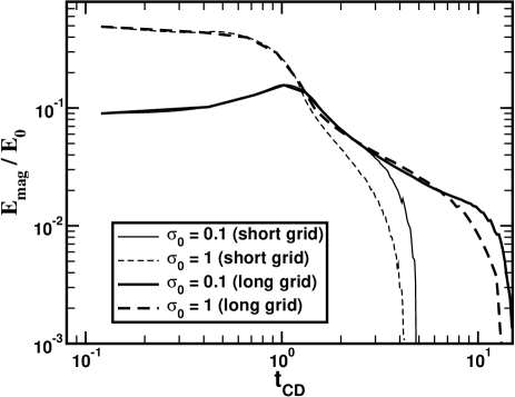
Figure 1: Magnetic energy fraction as function of the dimensionless observer time $t_{\rm CD}$. Thin lines show results for thin shell models $\sigma_{0}=0.1$ and $\sigma_{0}=1$ with the short grid, while the thick lines show results for the long grid. The rapid drop of the magnetic energy at late times is not physical but due to the fact that the whole magnetized shell leaves our computational box. This problem is ameliorated in the long grid models, where it shows up at later times, when the magnetic energy content is much smaller.

The remapping technique we are using to track the evolution of the shell consists in adding a certain number of numerical zones in front of the leading forward shock. The same number of zones is removed from the rear part of the domain. Since the shell is ultrarelativistic, the rear boundary is causally disconnected from the RS during the time in which we evolve our models. Thus, even considering that a part of the shell is lost through the rear radial boundary, for the purpose of computing the dynamics (or the emission) of the leading forward and reverse shocks, it suffices a relatively small computational domain $L$ spanning not only the shell, but a small portion of the leading and of the trailing medium, namely $L=1.5\Delta_{0}$ ($L=4\Delta_{0}$) for the thick (thin) shell models. However, due to the loss of the rear part of the shell, the calculation of any integral quantity extending over the whole shell (in particular the magnetic energy) is underestimated. To ameliorate such a deficiency of our models, we have computed some of the ”thin shell” simulations with a $\sim 3$ times larger grid (“long grid” in Fig. 1) than that used in MGA09 (“short grid” in Fig. 1). At $t_{\rm CD}<1$ the magnetic energy changes little (and actually increases in the $\sigma_{0}=0.1$ run because of the (reverse) shock compressing the ejecta). The magnetic energy drops fast at $t_{\rm CD}\sim 1$ because of the rarefaction that follows. Nevertheless, a fraction of $\sim 10$% of the total energy remains in magnetic form for longer time showing only modest decline with time (note that the large grid is essential to follow this late evolution). We find that at least $\sim 2\%$ of the energy in still in magnetic form at $t_{\rm CD}\sim 10$ (i.e., about 10 times the burst duration). The rapid drop of the magnetic energy at late times is not physical. It is due to the fact that the contact discontinuity reaches the back of our grid and the whole magnetized shell leaves our computational box (and we are left with the shocked ISM).

In view of these results, we suggest that there is sufficient energy remaining in the magnetic field for at least $\sim 10$ times the duration of the burst to yield a substantial emission if a large part of the magnetic energy is dissipated and radiated away.

5 Light curves and spectra

In this section we present the non-thermal light curves and spectra computed from our models. We first discuss the generic light curves corresponding to thin and thick shells for different magnetization of the ejecta. We also show a prototype emission spectrum at the end of this section.

5.1 Thin shells

Figure 2 shows the R-band light curves for the thin shell (i.e., $\xi=1.1$) model with initial magnetization $\sigma_{0}=0.01$ and bulk Lorenz $\Gamma_{0}=300$. The emission from the shocked external medium (thin full line), shocked ejecta (dotted line) and the total emission (thick full line) is displayed. We have assumed $\epsilon_{B}=5\times 10^{-3}$ and $\epsilon_{e}=10^{-1}$ so as to calculate emission. The total R-band light curves for models with different values $\sigma_{0}$ from $0$ to $1$ are shown in Fig. 3.

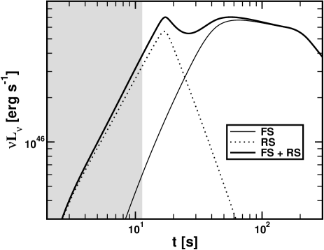
Figure 2: R-band light curve for the thin shell with initial magnetization $\sigma_{0}=0.01$. Shown are the light curves originating from the FS (thin full line), RS (dotted line) and the combined light curve (thick full line). In the calculation $\epsilon_{B}=5\times 10^{-3}$, $\epsilon_{e}=10^{-1}$ and the electron power-law index $p=2.25$. The shaded area denotes the observational interval which is simultaneous with the prompt emission.

As can be seen in Fig. 2 and, in general, in Fig. 3, for the parameters chosen the RS emission is marginally brighter than that of the FS in optical bands. Moderate differences in light curves for $t\mathbin{\lower 3.0pt\hbox{$\hbox to0.0pt{\raise 5.0pt\hbox{$\char 60\relax$}\hss}\mathchar 29208\relax$}}25\,$s are caused by the effect of $\sigma_{0}$ on the RS emission. Increasing $\sigma_{0}$ from $0$ to $0.01$ leads to progressively brighter RS emission because of increased synchrotron emissivity resulting from a stronger field. Further increase of the magnetization greatly weakens the RS emission and the amount of heating that takes place at the shock (and, therefore, reduces the electron minimum Lorenz factor in the downstream fluid; see Eq. 1) resulting in a negligible optical emission compared to that of the FS.

The FS emission shows a weak dependence on $\sigma_{0}$, the differences being more pronounced at higher energies (X-rays, gamma-rays) as shown in Fig. 4. Our models display an achromatic break in the light curves shortly after the end of the burst. The break takes place at $t\sim 30\,$s and $20\,$s for the $\sigma_{0}=0$ and $\sigma_{0}=1$ models, respectively, and it results from the rarefaction that reaches the FS and decelerates it. At early times, the emission in gamma- and X-rays is systematically brighter and flatter for high-$\sigma_{0}$ models than in the optical band, while the gamma- and X-ray flux rises faster for low-$\sigma_{0}$ models. Observing early enough after the burst, the high-energy emission from the FS can contain a valuable information about the magnetization of the ejecta. If the afterglow is observed too late, in this example after approximately $30\,$s(Fig. 4), light curves with radically different values of $\sigma_{0}$ become indistinguishable, since the ejecta enters into the self-similar evolution phase, dependent only on the total initial energy and the external medium density, which are the same for all models.

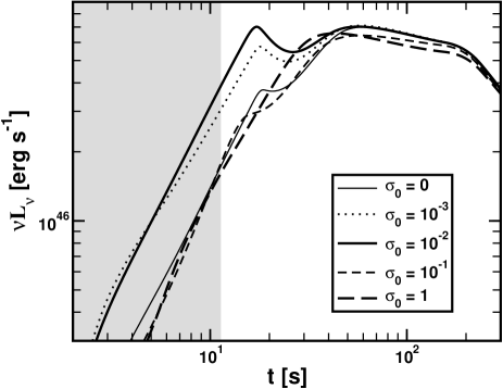
Figure 3: Combined (FS + RS) R-band light curves for thin shell models with $\sigma_{0}=0,\ 10^{-3},\ 10^{-2},\ 10^{-1}$ and $1$ (thin full, dotted, thick full, thin dashed and thick dashed lines, respectively). The rest of the parameters are like in Fig. 2.

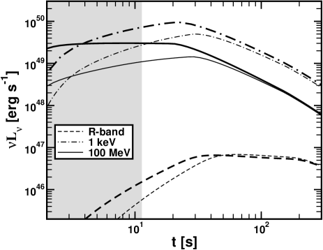
Figure 4: Forward shock emission. R-band, $1\,$keV and $100\,$MeV light curves (full, dotted and dashed lines, respectively) for thin shell models with $\sigma_{0}=0$ (thin lines) and $\sigma_{0}=1$ (thick lines).

5.2 Thick shells

We, now turn to the emission from a thick shell ($\xi=0.5$) for $\Gamma_{0}=750$. Figure 5 shows the contributions from the FS and the RS to the total R-band light curve for the model with initial magnetization $\sigma_{0}=0.01$. We can see that the RS the contribution to the emitted flux here is much more important than in the thin shell case. The RS dominates the emission until $t\simeq 50\,$s.

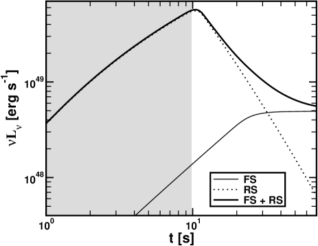
Figure 5: Same as Fig. 2 but for the thick shell with initial magnetization $\sigma_{0}=0.01$.

As can be seen in Fig. 6, the RS emission dominates in the early afterglow over that of the FS in the optical bands. Large differences in light curves for $t\mathbin{\lower 3.0pt\hbox{$\hbox to0.0pt{\raise 5.0pt\hbox{$\char 60\relax$}\hss}\mathchar 29208\relax$}}50$ s are caused by the effect of the magnetization $\sigma_{0}$ on the RS emission. For $\sigma_{0}=0$, there is a clear RS signature. It results from the synchrotron emission of non-thermal particles gyrating in the stochastic magnetic field (presumably) generated at the shocks. Increasing $\sigma_{0}$ from $0$ to $0.01-0.1$ leads to brighter RS (synchrotron) emission because of the stronger (shock compressed) magnetic field. Maximal RS emission happens for $\sigma_{0}\sim 0.01-0.1$. Around such values of $\sigma_{0}$ there is a turnover of the emission, which drops as the magnetization keeps growing. In effective terms, the RS light curve changes only moderately for $10^{-3}\mathbin{\lower 3.0pt\hbox{$\hbox to0.0pt{\raise 5.0pt\hbox{$\char 60\relax$}\hss}\mathchar 29208\relax$}}\sigma_{0}\mathbin{\lower 3.0pt\hbox{$\hbox to0.0pt{\raise 5.0pt\hbox{$\char 60\relax$}\hss}\mathchar 29208\relax$}}0.1$, and hence, inferring an accurate value of $\sigma_{0}$ from a careful modeling of the RS emission is difficult. Further increase of the magnetization greatly weakens the reverse shock and suppresses the energy injected to the particles. As a result, there is a clear suppression of the reverse shock emission for $\sigma_{0}\sim 1$ or higher.

Other mild differences in the optical lightcurves are caused by differences in the Lorenz factor of the FS at early times because of the different $\sigma_{0}$ as shown in Fig. 7. The thick-shell models show the same achromatic break in the light curves shortly after the end of the burst as seen in the thin shell ones. In this example, after approximately $30\,$s, FS light curves become indistinguishable, since the ejecta evolution approaches to the self-similar evolution phase.

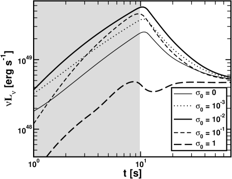
Figure 6: Same as Fig. 3, but for thick shell models.

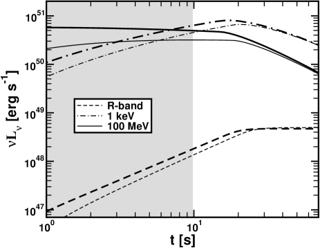
Figure 7: Same as Fig. 4, but for thick shell models.

5.3 Emission spectra

The instantaneous spectrum of the thick shell model $\sigma_{0}=0.01$ taken at $t=10\,$s is shown in Fig. 8. This time approximately corresponds to the peak of the RS emission and to the end of the prompt ($\sim$MeV) emission.

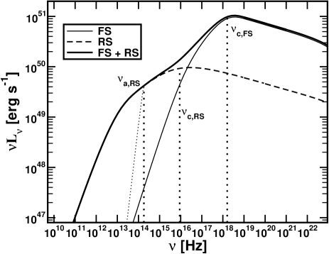
Figure 8: Emission spectrum at $t=10\,$s for the thick shell model with $\sigma_{0}=0.01$. Thin, full and dashed lines show optically thin FS and RS spectra, respectively. Thick full line shows the total spectrum. Thin dotted line shows the portion of the RS spectrum which is optically thick to synchrotron self-absorption (see text for details). Vertical dotted lines denote FS and RS cooling break frequencies $\nu_{\rm c,FS}$ and $\nu_{\rm c,RS}$, as well as the RS synchrotron-self absorption break frequency $\nu_{\rm a,RS}$.

Thick full line shows the total spectrum, while thin full and dashed lines show the FS and RS contributions, respectively. Both spectra have been computed neglecting the synchrotron self-absorption (SSA). Thin dotted line shows the RS spectrum when SSA is taken into account.

The peak of the $\nu L_{\nu}$ emission produced by each of the shocks corresponds to their respective cooling break frequencies. It appears in the X-ray band and in the UV band for the FS and RS, respectively. In Fig. 8 we also show the frequency of the SSA break for the reverse shock emission ($\nu_{\rm a,RS}$) that lies in the infra-red. Not surprisingly, the optical emission in the range $\sim 10^{14}-10^{15}\,$Hz is dominated by the RS, while the X-ray-to-$\gamma$-ray emission is dominated by the FS.

In deriving these results, we have assumed that electrons are accelerated into a power law distribution at the shocks. Despite the fact that particle acceleration in (relativistic) shocks is poorly understood, there are indications that strong, large scale fields along the shock plane can inhibit particle acceleration. For instance recent PIC simulations by Sironi & Spitkovsky (2009) have shown that for $\sigma\mathbin{\lower 3.0pt\hbox{$\hbox to0.0pt{\raise 5.0pt\hbox{$\char 62\relax$}\hss}\mathchar 29208\relax$}}0.01$, magnetized, relativistic shocks result in efficient heating of the particles with the distribution lacking non-thermal tails. If this result holds for the mildly relativistic shock forming in the ejecta, such lack on high-energy tail can substantially affect the RS emission (and, as a matter of fact, any emission from internal shocks). If the characteristic frequency (associated to the thermal distribution of the particles) lies bellow the observed band then there will be practically no observed emission from the RS. When the characteristic frequency of the RS emission (as is often the case) lies in the infrared, bursts of sufficiently high $\sigma_{0}\mathbin{\lower 3.0pt\hbox{$\hbox to0.0pt{\raise 5.0pt\hbox{$\char 62\relax$}\hss}\mathchar 29208\relax$}}0.01$ will be optically dim (there are no electrons accelerated to high enough energy to (synchrotron) emit in the optical or harder bands). This is an additional potential mechanism that suppresses the RS emission in moderately to strongly magnetized ejecta.

6 Application to GRB 990123 and GRB 090102

In this section we apply our early afterglow models to two specific GRBs exhibiting bright optical emission which may be powered by a reverse shock, GRB 990123 (Briggs et al., 1999; Akerlof & et al., 1999) and GRB 090102 (Gendre et al., 2009; Steele et al., 2009). The famous GRB 990123 had a 9th magnitude optical flare a few seconds after the end of the GRB and is one of the brightest ever detected. 090102 is a rather bright GRB whose early optical afterglow shows declining, but bright emission (Gendre et al., 2009) and, most importantly, a significant $\sim 10\%$ polarization, indicating large scale fields in the emitting region (Steele et al., 2009).

Several of the parameters of our model can be directly inferred by the observed properties of these bursts. The rest-frame duration of both bursts is $T_{\rm GRB}\simeq 10\,$s, constraining the shell thickness to be $\Delta_{0}\simeq cT_{\rm GRB}\simeq 3\times 10^{11}\,$cm. The gamma-ray fluence of GRB 990123 and 090102 is $E_{\gamma}\simeq 3\times 10^{54}\,$erg and $E_{\gamma}\simeq 6\times 10^{53}\,$erg, respectively. Assuming $\sim 20\%$ efficiency for the prompt emission mechanism the total (isotropic equivalent) energy of the ejecta can be estimated to be $E_{990123}\simeq 1.5\times 10^{55}$ erg and $E_{090102}\simeq 3\times 10^{54}$ erg. Finally, the fact the the reverse shock peaks very shortly after the burst indicates that $\xi\mathbin{\lower 3.0pt\hbox{$\hbox to0.0pt{\raise 5.0pt\hbox{$\char 60\relax$}\hss}\mathchar 29208\relax$}}1$ in these bursts.

Taking these observational constraints into account, we look for the values $\Gamma_{0}$ and $\sigma_{0}$ for which our rescaled numerical models best fit the observations. Figure 9 shows the R-band light curves of GRB 990123 (circles) and GRB 090102 (triangles). We also plot the light curves of two thick shell models, the $\sigma_{0}=0.01$ rescaled to $\Gamma_{0}=640$ (thick lines) and $\sigma_{0}=0.1$ rescaled to $\Gamma_{0}=940$ (thin lines). Full, dot-dashed and dashed lines denote the total, RS, and FS emission. The data in our simulation only allowed us to compute the FS emission up to $t\simeq 80\,$s. By this time, however, the evolution of the blast is self-similar. For the purpose of better visualization, we have used the Blandford-McKee asymptotic solution to extend the FS light curve to later times.

Even though our best fits suggest that $\sigma_{0}=0.1$ and $\sigma_{0}=0.01$ for GRBs 090102 and 990123 respectively, $\sigma_{0}$ is not well constrained. From Fig. 6, one can see that the RS emission varies relatively little for a large range of $0.01\mathbin{\lower 3.0pt\hbox{$\hbox to0.0pt{\raise 5.0pt\hbox{$\char 60\relax$}\hss}\mathchar 29208\relax$}}\sigma_{0}\mathbin{\lower 3.0pt\hbox{$\hbox to0.0pt{\raise 5.0pt\hbox{$\char 60\relax$}\hss}\mathchar 29208\relax$}}0.1$ indicating that pinpointing the magnetization with precision from fitting the reverse shock light curve is hard.

The optical afterglow of GRB 090102 shows $\sim 10$% polarization at an exposure that took place $160-220\,$s after the GRB trigger (Steele et al., 2009). This value is very hard to understand as synchrotron emission from small scale magnetic fields but is still smaller than that expected from a coherent field. The exposure time interval of the Steele et al. (2009) observations corresponds to the time interval $100-140\,$s in the frame of the source. One can see in Fig. 9 that at $\sim 100\,$s the FS emission may already dominate over the RS emission by a modest factor. The observed 10% polarization may, therefore, be understood as a combination of the very weekly polarized, brighter FS emission and a strongly polarized emission coming from RS that propagates in a flow of coherent field. If this interpretation is correct, earlier polarimetry of afterglow emission should reveal even stronger polarization signal, for these few bursts for which the RS emission is sufficiently bright with respect to the FS.

Another intriguing result from the fitting of our models is that, in order for the FS to account for the late-time emission, a rather small value of $\epsilon_{B}\sim 10^{-7}$ needs to be assumed. For GRB 990123, a similar finding is presented in Panaitescu & Kumar (2004). Note that such weak fields may be simply due to shock compression of the ISM magnetic fields (i.e., there is no need for field generation at the shocks for these bursts). Kumar & Duran (2009) present more bursts whose afterglow modeling is compatible with very low values of $\epsilon_{B}$.

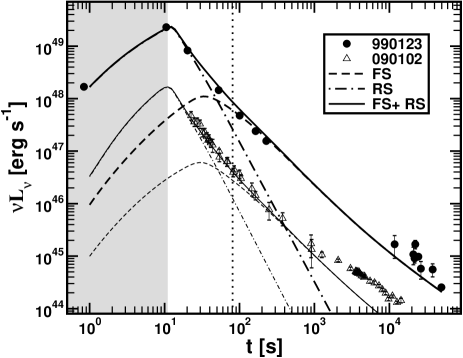
Figure 9: R-band light curve for GRB 990123 (Briggs et al., 1999; Akerlof & et al., 1999), GRB 090102 (Gendre et al., 2009; Steele et al., 2009) plotted in the rest frame of the central engine of the burst. Shown are the thick shell models which most closely match the observed light curves, assuming for both bursts ejecta width $\Delta_{o}=3.3\times 10^{11}\,$cm (with corresponding duration of $11$ seconds; marked by the shaded region in the plot). The $\sigma_{0}=0.01$ model (thick lines) has been rescaled to $\Gamma_{0}=640$ and $n_{\rm ext}=10\,$cm^-3. The $\sigma_{0}=0.1$ model (thin lines) has been rescaled to $\Gamma_{0}=940$, $n_{\rm ext}=1$ cm^-3. For both curves $\epsilon_{e}=0.02$ and $\epsilon_{B}=4\times 10^{-7}$ are assumed. Full, dot-dashed and dashed lines denote the total (FS + RS), RS and, FS emission. The vertical dotted line shows the observer time up to which the data from the simulation has been used to compute the FS emission; from that point onwards the Blandford-McKee asymptotic solution has been used to compute the FS light curve.

7 Discussion and conclusion

The theoretical modeling of GRB central engines is still far from predicting whether the GRB flow is thermally or magnetically dominated in the launching region. Furthermore, prompt GRB emission mechanisms are not understood well enough to enable probing of the magnetization of the emitting plasma. A more promising way to infer the magnetization of the GRB flow may come through studying interactions with the circumburst medium. Quantitative inferences, however, critically depend upon the detailed modeling of the dynamics of such interaction, as well as the emission mechanisms from shocked plasma. In this work we presented relativistic MHD models of ejecta-medium interactions coupled to a radiative transfer code to calculate multi-wavelength synchrotron lightcurves. The most salient results of our parametric study are the following:

1. For very weakly magnetized ejecta, the standard forward/reverse shock structure (Sari & Piran, 1995) is reproduced by our simulations. The reverse shock can dominate the early optical/IR emission while the forward shock dominates the subsequent emission at all wavelengths. Increasing the magnetization of the ejecta to $\sigma_{0}\sim 0.01-0.1$, the reverse shock remains strong while the powerful fields result in a brighter synchrotron emission, typically, in the optical band. At still stronger magnetization $\sigma_{0}\mathbin{\lower 3.0pt\hbox{$\hbox to0.0pt{\raise 5.0pt\hbox{$\char 62\relax$}\hss}\mathchar 29208\relax$}}1$, the dissipation at the reverse shock and, therefore its emission are greatly reduced.

2. Observationally, the majority of GRBs do not show bright optical emission at early times. Klotz et al. (2009) present a systematic study of early optical observations and tight upper limits tens of seconds after GRB emission. We interpret this lack of early optical detections as evidence for weak/absent reverse shock as expected from GRB flows characterized by $\sigma_{0}\mathbin{\lower 3.0pt\hbox{$\hbox to0.0pt{\raise 5.0pt\hbox{$\char 62\relax$}\hss}\mathchar 29208\relax$}}1$ at large distance from the central engine. Nevertheless, a few GRBs such as 990123 and 090102 do show bright optical emission that is likely coming from the reverse shock (Akerlof & et al., 1999; Mészáros & Rees, 1999; Nakar & Piran, 2005; Steele et al., 2009).

3. Our detailed modeling of early afterglow emission from GRB 990123 and 090102 indicates that the magnetization of the ejecta is $\sigma_{0}\sim 0.01-0.1$ for these bursts, i.e., close to the value that maximizes the RS brightness (see Fig. 9). For GRB 090102, the presence of a large scale field is strongly supported by the detection of $\sim 10$% optical polarization (Steele et al., 2009) during a $60\,$s exposure shortly after the burst. It, therefore, appears that there is a range of magnetizations of $\sigma_{0}>0.01-0.1$ for the GRB ejecta at the radius of deceleration. This values are compatible with super-fast magnetosonic MHD models for GRBs.

4. The reverse shock slows down and compresses the shell. As a result, during the RS crossing the magnetic energy of the ejecta is actually increased (Zhang & Kobayashi, 2005, MGA09). Subsequently, the bulk of the magnetic energy is diluted because of a rarefaction that crosses the ejecta (produced when the RS reaches the innermost radial edge of the ejected shell). The remaining ($\sim$10%) of the magnetic energy decays slowly with time (see Fig. 1). If a substantial fraction of this energy is radiated away because of dissipative MHD processes (Giannios, 2006), it may account for the X-ray flares observed minutes to hours after many GRBs (Burrows & et al., 2005).

5. The bulk of the magnetic energy is transferred into the shocked ISM shortly after the end of the burst. Only at this point, the blast wave establishes the well known BM self-similar behavior. A flat or rising light curve until well after the GRB is over at high-energies is the signature imprinted on the FS emission by the aforementioned energy transfer. An initially flat high-energy light curve may be the signature of $\sigma_{0}\sim 1$ ejecta while a rising one comes from smaller magnetization (assuming always a constant density ISM). When the energy transfer is completed, an achromatic break takes place. After the break, the light curve declines as expected from the BM solution.

6. It has been proposed (Kumar & Duran, 2009; Ghisellini et al., 2010) that the GeV emission observed by the LAT detector on FERMI in several bursts is result of the FS. The model can account for GeV observations shortly after the end of the burst and and for the late optical and X-ray data. In its simplest form, however, the FS model cannot explain the peak of the GeV emission at times $t_{peak}<t_{\rm GRB}$ seen in GRB 080916C, 090510 and likely in 090902B (since, as we have shown here, the energy transfer to the FS results in $t_{peak}\mathbin{\lower 3.0pt\hbox{$\hbox to0.0pt{\raise 5.0pt\hbox{$\char 62\relax$}\hss}\mathchar 29208\relax$}}t_{\rm GRB}$). On the other hand, from the Ghisellini et al. (2010) sample of several LAT bursts, at least three GRBs (090323, 090626, and 091003) show a rather flat GeV light curve that steepens only after the MeV emission (i.e. the traditional GRB) is over. Though more detailed modeling is needed, the emission from these bursts appears compatible with coming from the early FS driven by ejecta with $\sigma_{0}\geq 1$ in agreement with inferences we have made from the lack of observed of RS emission.

The results outlined so far suggest that to explain the paucity of observed optical flashes one needs to argue that most of the observed bursts posses substantial magnetizations (point (ii) above). However, our models are sensitive to a number of parameters, among which, $\epsilon_{B}$ is probably the most crucial one. The value that we use as representative in our models ($\epsilon_{B}\sim 5\times 10^{-3}$; Sect. 5) results in powerful optical flashes even for the $\sigma_{0}=0$ model. Values of $\epsilon_{B}\ll 5\times 10^{-3}$ reduce the strength of the RS emission. We find that for $\epsilon_{B}\mathbin{\lower 3.0pt\hbox{$\hbox to0.0pt{\raise 5.0pt\hbox{$\char 60\relax$}\hss}\mathchar 29208\relax$}}10^{-6}-10^{-5}$ the RS emission falls below that of the FS, for all our purely hydrodynamic models ($\sigma_{0}=0$). Therefore, even in fireball models one may argue that the optical emission of the RS is suppressed if mildly relativistic shocks are not able to efficiently generate stochastic magnetic fields.

Another issue that has to be taken into consideration is the fact that we are modeling the ejecta as initially being cold. Moderately hot or warm ejecta (i.e., in which $P/\rho c^{2}\mathbin{\lower 3.0pt\hbox{$\hbox to0.0pt{\raise 5.0pt\hbox{$\char 60\relax$}\hss}\mathchar 29208\relax$}}1$) may result, e.g., if the conversion of internal to kinetic energy is slower than predicted by the standard fireball model (which might not be unlikely by looking at the numerical models of, e.g., Aloy et al. 2000; Aloy et al. 2005), or if internal shocks heat up the ejecta shortly before the reverse shock crossing. In such scenario, a weaker RS may be envisioned, since it is more difficult to shock warm than cold matter. Thus, we may not exclude the possibility that the absence of a clear RS signature in many GRBs arises (assuming that the ejecta is not magnetized) from the fact that the ejecta is warm by the time the afterglow emission takes place.

References

- Akerlof & et al. (1999) Akerlof C., et al.1999, Nature, 398, 400
- Aloy et al. (1999) Aloy M. A., et al., 1999, ApJS, 122, 151
- Aloy et al. (2005) Aloy M. A., et al., 2005, A&A, 436, 273
- Aloy & Mimica (2008) Aloy M. A., Mimica P., 2008, ApJ, 681, 84
- Aloy et al. (2000) Aloy M. A., et al., 2000, ApJ, 531, L119
- Aloy & Obergaulinger (2007) Aloy M. A., Obergaulinger M., 2007, RMxAC 30, 96
- Blandford & McKee (1976) Blandford R. D., McKee C. F., 1976, Physics of Fluids, 19, 1130
- Briggs et al. (1999) Briggs M. S., et al., 1999, ApJ, 524, 82
- Burrows & et al. (2005) Burrows D. N., et al.2005, Science, 309, 1833
- Dermer (2008) Dermer C. D., 2008, ApJ, 684, 430
- Drenkhahn & Spruit (2002) Drenkhahn G., Spruit H. C., 2002, A&A, 391, 1141
- Fan et al. (2002) Fan Y.-Z., et al., 2002, Chinese J. of Astron. & Astroph., 2, 449
- Fan et al. (2008) Fan Y.-Z., et al., 2008, MNRAS, 384, 1483
- Fan et al. (2004a) Fan Y. Z., Wei D. M., Wang C. F., 2004a, A&A, 424, 477
- Fan et al. (2004b) Fan Y. Z., et al., 2004b, MNRAS, 354, 1031
- Gendre et al. (2009) Gendre B., et al., 2009, arXiv:0909.1167
- Genet et al. (2006) Genet F., et al., 2006, A&A, 457, 737
- Ghisellini et al. (2010) Ghisellini G., et al., 2010, MNRAS, 403, 926
- Giannios (2006) Giannios D., 2006, A&A, 455, L5
- Giannios (2008) Giannios D., 2008, A&A, 480, 305
- Giannios et al. (2008) Giannios D., et al., 2008, A&A, 478, 747
- Giannios & Spitkovsky (2009) Giannios D., Spitkovsky A., 2009, MNRAS, 400, 330
- Goodman (1986) Goodman J., 1986, ApJL, 308, L47
- Granot et al. (2001) Granot J., et al., 2001, proceedings of the conference “Gamma-Ray Bursts in the Afterglow Era”, Rome, Italy 17-20 October 2000, pp 312
- Granot et al. (1999) Granot J., et al., 1999, ApJ, 513, 679
- Klotz et al. (2009) Klotz A., et al., 2009, AJ, 137, 4100
- Kobayashi et al. (1999) Kobayashi S., et al., 1999, ApJ, 513, 669
- Komissarov et al. (2009) Komissarov S. S., et al., 2009, MNRAS, 394, 1182
- Kumar & Duran (2009) Kumar P., Duran R. B., 2009, MNRAS, 400, L75
- Leismann et al. (2005) Leismann T., et al., 2005, A&A, 436, 503
- Li et al. (1992) Li Z.-Y., et al., 1992, ApJ, 394, 459
- Lyubarsky (2010) Lyubarsky Y. E., 2010,MNRAS, 402, 353
- Lyutikov (2005) Lyutikov M., 2005, arXiv:astro-ph/0503505
- Lyutikov (2006) Lyutikov M., 2006, New Journal of Physics, 8, 119
- Lyutikov & Blandford (2003) Lyutikov M., Blandford R., 2003, ArXiv:astro-ph/0312347
- McMahon et al. (2006) McMahon E.,et al., 2006, MNRAS, 366, 575
- Meliani et al. (2007) Meliani Z., et al., 2007, MNRAS, 376, 1189
- Meszaros & Rees (1997) Meszaros P., Rees M. J., 1997, ApJ, 482, L29
- Mészáros & Rees (1999) Mészáros P., Rees M. J., 1999, MNRAS, 306, L39
- Mimica & Aloy (2010) Mimica P., Aloy M. A., 2010, MNRAS, 401, 525
- Mimica et al. (2009a) Mimica P., et al., 2009a, ApJ, 696, 1142
- Mimica et al. (2007) Mimica P., et al., 2007, A&A, 466, 93
- Mimica et al. (2005) Mimica P., et al., 2005, A&A, 441, 103
- Mimica et al. (2009b) Mimica P., et al., 2009b, A&A, 494, 879
- Mizuno et al. (2009) Mizuno Y., et al., 2009, ApJ, 690, L47
- Nakar & Piran (2004) Nakar E., Piran T., 2004, MNRAS, 353, 647
- Nakar & Piran (2005) Nakar E., Piran T., 2005, ApJ619, L147
- Paczynski (1986) Paczynski B., 1986, ApJL, 308, L43
- Panaitescu & Kumar (2004) Panaitescu A., Kumar P., 2004, MNRAS, 353, 511
- Petropoulou & Mastichiadis (2009) Petropoulou M., Mastichiadis A., 2009,A&A, 507, 599
- Rees & Meszaros (1992) Rees M. J., Meszaros P., 1992, MNRAS, 258, 41P
- Rees & Meszaros (1994) Rees M. J., Meszaros P., 1994, ApJL, 430, L93
- Sari & Piran (1995) Sari R., Piran T., 1995, ApJL, 455, L143
- Sironi & Spitkovsky (2009) Sironi L., Spitkovsky A., 2009, ApJ, 698, 1523
- Spitkovsky (2008) Spitkovsky A., 2008, ApJ, 682, L5
- Spruit et al. (2001) Spruit H. C., et al., 2001, A&A, 369, 694
- Steele et al. (2009) Steele I. A., et al., 2009, Nature, 462, 767
- Tchekhovskoy et al. (2009) Tchekhovskoy A., et al., 2009, ApJ, 699, 1789
- Thompson (1994) Thompson C., 1994, MNRAS, 270, 480
- Usov (1992) Usov V. V., 1992, Nature, 357, 472
- van Eerten et al. (2010) van Eerten H. J., et al., 2010, MNRAS, 403, 300
- Zhang & Kobayashi (2005) Zhang B., Kobayashi S., 2005, ApJ, 628, 315
- Zhang et al. (2003) Zhang B., et al., 2003, ApJ, 595, 950