Chemical Oscillations out of Chemical Noise

Abstract

The dynamics of one species chemical kinetics is studied. Chemical reactions are modelled by means of continuous time Markov processes whose probability distribution obeys a suitable master equation. A large deviation theory is formally introduced, which allows developing a Hamiltonian dynamical system able to describe the system dynamics. Using this technique we are able to show that the intrinsic fluctuations, originated in the discrete character of the reagents, may sustain oscillations and chaotic trajectories which are impossible when these fluctuations are disregarded. An important point is that oscillations and chaos appear in systems whose mean-field dynamics has too low a dimensionality for showing such a behavior. In this sense these phenomena are purely induced by noise, which does not limit itself to shifting a bifurcation threshold. On the other hand, they are large deviations of a short transient nature which typically only appear after long waiting times. We also discuss the implications of our results in understanding extinction events in population dynamics models expressed by means of stoichiometric relations.

1 Introduction

The kinetics of reaction systems have been extensively studied over the years. These systems have been postulated as paradigmatic models for the description of a large number of natural phenomena, including topics from organic and inorganic chemistry, epidemiology, population biology and genetics, nuclear physics, non-equilibrium statistical mechanics and many others sciences [1, 2]. The mathematical description of such systems usually starts with the assumption of a set of stoichiometric relations of the form

$$A\stackrel{{\scriptstyle\alpha}}{{\longrightarrow}}B,$$ (1)

signifying that the reagent $A$ transforms to $B$ with the time dependent probability

$$P_{A\to B}(t)=\alpha e^{-\alpha t},$$ (2)

where $\alpha>0$ is the specific reaction rate. Note that the probabilistic nature of the reactions introduces fluctuations into the dynamics: this is the “chemical noise” we will be interested in. In more general terms, the state of a system containing $m$ reagents and $n$ reactions is described by a continuous time Markov process. All the available information is carried by the distribution $P(n_{A},n_{B},\cdots;t)$ specifying the probability of the existence of exactly $n_{A}$ reagents of type $A$, $n_{B}$ of type $B$, …, at time $t$. The dynamics of this distribution is governed by a master equation of the form [1, 2]

$$\frac{dP_{k}}{dt}=\sum_{j\neq k}\left[W_{j\to k}P_{j}-W_{k\to j}P_{k}\right],$$ (3)

where $P_{k}$ denotes the probability of finding the system in the state $k$ characterized by a certain number of reagents of each type, and $W_{j\to k}$ is the transition matrix from state $j$ to state $k$. While solving the master equation to find $P_{k}$ would mean that we possess all the available information on the system, the chances of obtaining an exact closed form for $P_{k}$ are scarce in realistic situations. Additionally, the amount of information it brings is usually excessive, and a great part of it does not add any valuable information about the dynamics. Consequently, the most common approach to the subject concentrates on the dynamics of some statistical quantity of interest, as for instance a density, which is able to describe the system macroscopic state. The selection of an adequate variable has to be supplemented with selecting a suitable approximation in order to get an operative theory that allows studying the otherwise commonly untractable master equation. A particularly advantageous choice is the analog of the quantum mechanical Wentzel-Kramers-Brillouin (WKB) approximation adapted to this sort of systems, which is now well established in both physical and mathematical literatures, see for instance [3, 4, 5, 6, 7, 8, 9, 10, 11, 12, 13, 14, 15]. It allows the description of both the short time dynamics, which is to a large extent independent of the fluctuations and therefore captured by mean-field type approximations, and the long time behavior which is affected, dramatically on occasion, by large deviations. The mathematical and physical natures of these large deviations will appear clearer in the following sections.

In this work we are concerned with simple reaction sets which on the other hand have an intuitive physical meaning. This way we will focus on simplified model systems which, although not of direct practical applicability, facilitate analytic progress and physical intuition. We will show how chemical fluctuations strongly affect the dynamics for long times, when large deviations have had time to develop. In these cases, chemical fluctuations are able to promote periodic orbits and chaotic behavior in reaction systems whose dimensionality is too low to present such a behavior if strictly deterministic dynamics are considered. These effects are, however, both rare and short-lived. They are, at the same time, substantially different from other sorts of noise-induced oscillations which appear in different important phenomena and whose structure relies on an existing deterministic mechanism (like the proximity to a deterministic bifurcation) which is anticipated or activated by noise [16, 17, 18, 19, 20]. In this sense, we may say our focus is on oscillations which are purely promoted by chemical noise. Our approach will be probabilistic at the beginning, when we will present formal calculations in which the equations governing large fluctuations will be derived. These equations have the form of Hamiltonian dynamical systems, which will be in realistic situations genuinely different from the ones usually considered in classical mechanics. For them we will be able to show, by means of explicit calculations, rigorous proofs and numerical simulations, how chemical noise is capable of sustaining chemical oscillations, both of periodic and chaotic nature.

2 Large deviations

2.1 Brownian motion

We devote this section to clarify the type of problems we are going to solve. We start with the perhaps simplest stochastic process one could consider: one-dimensional Brownian motion. For our current purposes it will be the solution of the equation

$$\frac{dB}{dt}=D\,\xi(t),$$ (4)

where $D>0$ is a diffusion constant and $\xi(t)$ is the standard Gaussian white noise defined by its two first moments

$$\mathbb{E}[\xi(t)]=0,\qquad\mathbb{E}[\xi(t)\xi(t^{\prime})]=\delta(t-t^{\prime}),$$ (5)

where $\delta(\cdot)$ is the Dirac delta distribution. Of course, a rigorous interpretation of this equation is possible in terms of Itô calculus [21], but such a precise definition will not be needed herein. Equation (4) is provided with the initial condition $B(0)=0$. A classical problem within this subject is calculating the first time the random walker $B(t)$ reaches some fixed level $a\neq 0$ in absence of other constraints. The well–known solution states that the random walker reaches level $a$ in finite time with probability one, but the mean time at which this event occurs diverges.

Langevin equations like (4) and more complicated variants of it are well understood from the large deviations point of view [22]. It associates to this stochastic differential equation the rate or action functional

$$S[x(t)]=\frac{1}{2D}\int|\dot{x}(t^{\prime})|^{2}dt^{\prime},$$ (6)

which in the small noise limit $D\to 0$ gives rise to the following Euler-Lagrange equation

$$\ddot{x}=0,$$ (7)

for the position $x$ of the random walker. If we complement this equation with the boundary conditions $x(0)=0$ and $x(T)=a$ we find the solution

$$x(t)=\frac{a}{T}t,$$ (8)

signaling the most probable trajectory that links the origin with the level $a$ after a time $T$ for the Brownian dynamics (4). Small deviations are obtained by setting $D=0$ in (4). In this case the random walker stays at the origin for all times. So the full picture would be, for small noise, the random walker will be at a neighborhood of the origin with a large probability but with a small probability large deviations might appear and drive the system further away. The probability $\mathcal{P}$ with which these large deviations, which promote trajectories (8), manifest themselves into the system dynamics is proportional to the exponential of the negative of the action

$$\mathcal{P}\sim e^{-S}=\exp\left(-\frac{a^{2}}{2DT}\right).$$ (9)

From this formula it is clear that those trajectories that connect the origin with the level $a$ in a shorter time are rarer than those which take a longer time. The prefactor in this case is easily found by normalization. Note that the large deviation theory is valid for $a^{2}\gg DT$, otherwise the system diffuses away from the original position and the approximation breaks down.

2.2 Plankton extinction

We will describe now the large deviations technique in the context of reaction kinetics. To this end we consider a simple model that has nevertheless a genuine practical interest. This model was introduced as a description of plankton population dynamics [23, 24, 25] and nonequilibrium statistical mechanics [26]. It consists of the following reactions

$$A\stackrel{{\scriptstyle\gamma}}{{\longrightarrow}}2A,\qquad A\stackrel{{\scriptstyle\gamma}}{{\longrightarrow}}\emptyset,$$ (10)

happening at the same rate $\gamma$. We will employ large deviation theory to describe the extinction of the “plankton population” $A$. The state of the system may be described by a continuous time Markov process obeying the master equation

$$\frac{dP_{n}}{dt}=\gamma[(n-1)P_{n-1}-nP_{n}]+\gamma[(n+1)P_{n+1}-nP_{n}],$$ (11)

where the term inside the first bracket corresponds to the branching reaction and the one inside the second bracket to the disintegration reaction. By introducing the generating function

$$G(p,t)=\sum_{n=0}^{\infty}p^{n}P_{n}(t),$$ (12)

we transform the master equation into the following “imaginary time Schrödinger equation”

$$\partial_{t}G=\gamma(p-1)^{2}\partial_{p}G.$$ (13)

Note that we are employing the “momentum” rather than the “coordinate” representation in this last equation. One can obtain the probability distribution from the generating function in the following way

$$P_{n}(t)=\frac{1}{2\pi i}\oint G(p,t)\,p^{-n}\,\frac{dp}{p},$$ (14)

where the contour integral runs over a closed path on the complex $p-$plane, surrounding the origin and going through the region of analyticity of $G(p,t)$. The corresponding “classical” Hamiltonian of our theory reads

$$\mathcal{H}=\gamma(p-1)^{2}q;$$ (15)

it is precisely this Hamiltonian, as in the previous case, which describes the large deviations of the system. The corresponding equations of motion are

$$\dot{q} = \frac{\partial\mathcal{H}}{\partial p}=2\gamma(p-1)q,$$ (16)

$$\dot{p} = -\frac{\partial\mathcal{H}}{\partial q}=-\gamma(p-1)^{2}.$$ (17)

Note that the line $p=1$ is degenerate and all points on it are fixed points. These solutions refer to small deviations: the system stays with a large probability in a neighborhood of the initial condition for short times as in the Brownian motion case. The solution for the coordinate $q$ is

$$q(t)=\left(\sqrt{q(0)}\pm\sqrt{\gamma H}t\right)^{2},$$ (18)

where the minus sign is selected for extinction trajectories and $H$ is a constant indicating the initial “energy”. The duplicity of signs in this equation comes from the extraction of the square root of equation (15). The number $n$ of reagents can be calculated by means of formally applying a steepest descent approximation to formula (14) for $G(p,t)=\exp[-S(p,t)]$, where $S$ is the “classical” action [9]. Then one finds $n\approx-p\partial_{p}S$, and employing the “classical” relation $q=-\partial_{p}S$ one concludes $n(t)\approx p(t)q(t)$. In our particular example one finds

$$n\approx pq=q-\sqrt{\frac{Hq}{\gamma}},$$ (19)

which becomes zero due to a fluctuation when $p\to 0$, which leads to $q=H/\gamma$. If the system follows an optimal trajectory it will become extinct after a time

$$t_{e}=\sqrt{\frac{q(0)}{\gamma H}}-\frac{1}{\gamma}.$$ (20)

The probability with which this realization appears for short times is the exponentiated negative of the action $\mathcal{P}\sim e^{-S}$, up to some prefactor. We will limit ourselves to the exponential order, as the calculation of the prefactor is a rather technical issue [15] and will not add substantial information to the present discussion. The action reads

$$S=\int_{0}^{t_{e}}(p\dot{q}-H)dt+[p(0)q(0)-p(t_{e})q(t_{e})]+S_{0}=S_{0},$$ (21)

in the case of an extinction trajectory, where the initial action $S_{0}=-\ln[G(p,0)]$. The last equality has been derived employing the following derivations

$$\int_{0}^{t_{e}}(p\dot{q}-H)dt = \int_{0}^{t_{e}}[p\dot{q}-\gamma(p-1)^{2}q]dt=\int_{0}^{t_{e}}\gamma q(p^{2}-1)dt,$$ (22)

$$\frac{d}{dt}(pq) = \gamma q(p^{2}-1),$$ (23)

where we have substituted $\dot{p}$ and $\dot{q}$ for their respective values from (16) and (17). We consider two initial conditions as in [9], the Poisson distributed initial condition with average $n_{0}$, this is $G(p,0)=\exp[n_{0}(p-1)]$, and the Kronecker delta centered at $n_{0}$, which is $G(p,0)=p^{n_{0}}$. In the first case the extinction probability reads

$$\mathcal{P}\sim\exp\left[-\sqrt{\frac{H^{2}}{4\gamma^{2}}+\frac{Hn_{0}}{\gamma}}+\frac{H}{2\gamma}\right],$$ (24)

and in the second

$$\mathcal{P}\sim\left[1+\frac{H}{2n_{0}\gamma}-\sqrt{\frac{H^{2}}{4n_{0}^{2}\gamma^{2}}+\frac{H}{n_{0}\gamma}}\right]^{n_{0}},$$ (25)

and both yield the same result in the thermodynamic limit $n_{0}\to\infty$

$$\mathcal{P}\sim\exp\left(-\sqrt{\frac{Hn_{0}}{\gamma}}\right).$$ (26)

The optimal trajectory corresponding to this characteristic time to extinction is found by combining Eq. (18) (with the minus sign) and the expression for $n$ given by the second equality of Eq. (19)

$$n(t)=n_{0}+\gamma Ht^{2}-t\sqrt{H^{2}+4n_{0}\gamma H}\approx\left(\sqrt{n_{0}}-\sqrt{\gamma H}\,t\right)^{2},$$ (27)

where the thermodynamic limit $n_{0}\to\infty$ has been considered in the last step. In the derivation of the first equality we have employed the following two relations

$$n(t) = \left(n_{0}-\sqrt{\gamma Hq(0)}\,t\right)\left(1-\sqrt{\frac{\gamma H}{q(0)}}\,t\right),$$ (28)

$$\sqrt{q(0)}+\frac{n_{0}}{\sqrt{q(0)}} = \sqrt{\frac{H}{\gamma}+4\,n_{0}}.$$ (29)

Note that we have found a one parameter family of solutions, parameterized with the energy $H$. Time $t_{e}$ is not the mean extinction time, because at every time there are equally probable trajectories which do not become extinct, the ones corresponding to the plus sign in Eq. (18). This makes the mean extinction time infinite, although the system becomes extinct with probability one [2, 27]. The interpretation of this time is that of a characteristic time of extinction, this is, if the system becomes extinct after a time $t_{e}$ then the most probable path to extinction would have been (27). Note that more “energetic” trajectories lead to extinction faster but they are less probable. Using the relation between $t_{e}$ and $H$ we may find an expression akin to (9):

$$\mathcal{P}\sim\exp\left(-\frac{n_{0}}{\gamma t_{e}}\right).$$ (30)

Note that in this case the scaling is different. Note also that, as in the previous case, the large deviation theory that has led us to the optimal trajectories (27) is valid for short times $t\ll n_{0}/\gamma$.

3 Chemical oscillations and chaos

3.1 Noise induced oscillations

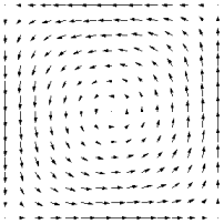
Figure 1: Vector field of the Hamiltonian system (36) (detail of the quadrangular area enclosed by the four zero energy lines). The values of the parameters are $\mu=1$ and $\sigma=2$.

We now move to studying the more complex nonlinear reversible reaction

$$A\stackrel{{\scriptstyle\mu}}{{\longrightarrow}}2A,\qquad 2A\stackrel{{\scriptstyle\sigma}}{{\longrightarrow}}A.$$ (31)

It is clear that it can be considered as a stochastic discrete model for logistic growth. The master equation describing this reactions set is

$$\frac{dP_{n}}{dt}=\mu[(n-1)P_{n-1}-nP_{n}]+\frac{\sigma}{2}[(n+1)nP_{n+1}-n(n-1)P_{n}].$$ (32)

We may use the generating function technique to convert this equation into a partial differential equation which can be exactly mapped, using quantum mechanical tools, into the path integral [9]

$$U=\int\mathcal{D}p\mathcal{D}qe^{-S[p,q]},$$ (33)

where $U$ is the problem Green function. The action reads

$$S[p,q]=\int_{0}^{t}\left[p\dot{q}-\mu(p^{2}-p)q-\frac{\sigma}{2}(p-p^{2})q^{2}\right]dt+[p(0)q(0)-p(t)q(t)]+S_{0},$$ (34)

and upon rendering the variables nondimensional $q\to(2\mu/\sigma)q$ (so this new $q=O(1)$, see below) and $t\to t/\mu$ one finds

$$S[p,q]=\frac{2\mu}{\sigma}\left\{\int_{0}^{t/\mu}\left[p\dot{q}-(p^{2}-p)q-(p-p^{2})q^{2}\right]dt+[p(0)q(0)-p(t)q(t)]+\tilde{S}_{0}\right\},$$ (35)

where $\tilde{S}_{0}=\sigma S_{0}/(2\mu)=O(1)$, so the steepest descent method makes sense for $\mu\gg\sigma$. In this approximation and recovering the dimensional coordinates the large deviations problem reduces to studying the Hamiltonian [11]

$$\mathcal{H}=\mu(p^{2}-p)q+\frac{\sigma}{2}(p-p^{2})q^{2},$$ (36)

and the corresponding dynamical system

$$\left\{\begin{aligned} \dot{p}&=&-\frac{\partial\mathcal{H}}{\partial q}=\mu(p-p^{2})+\sigma(p^{2}-p)q,\\ \dot{q}&=&\frac{\partial\mathcal{H}}{\partial p}=\mu(2p-1)q+\frac{\sigma}{2}(1-2p)q^{2}.\end{aligned}\right.$$ (37)

This system has five fixed points, four of which lie in the energy $H=0$ level, these are

$$(0,0),\quad(0,2\mu/\sigma),\quad(1,0),\quad\mathrm{and}\quad(1,2\mu/\sigma),$$ (38)

all of them are saddles. The fifth fixed point is $(1/2,\mu/\sigma)$, its energy is $H=-\mu^{2}/(8\sigma)$, and it is a local minimum of energy, what implies it is a center. The $H=0$ level is particularly simple, as it is composed of the four invariant lines

$$\{p=0\},\quad\{p=1\},\quad\{q=0\},\quad\mathrm{and}\quad\{q=2\mu/\sigma\}.$$ (39)

The dynamics is exactly integrable in all these lines. They cross at the four zero energy fixed points, and they enclose a quadrangular area in whose center lies the fifth fixed point. In this quadrangular area all the trajectories are periodic orbits surrounding the center, see Fig. 1. Note that, both outside and inside these four zero energy lines the energy is strictly negative. The mean-field behavior corresponds to the $\{p=1\}$ line, on which the dynamics reduces to the well known logistic equation

$$\dot{q}=\mu q-\frac{\sigma}{2}q^{2}.$$ (40)

As expected, reaction (31) corresponds to pure logistic growth when the fluctuations are neglected, this is, for a large number of reagents and short times. So at the mean-field level the only possibility is a monotonic approach to the stable fixed point $q=2\mu/\sigma$, provided the initial condition fulfills $q>0$. So the dynamical scenario presents a very reduced phenomenology in this case. However, if we consider the intrinsic fluctuations and thus the full phase space things are different. In this case, for instance, we may observe the system for a short time in the neighborhood of the fifth fixed point, which represents a reagent density $n\approx\mu/(2\sigma)$ (this is obtained as the product $pq$ evaluated at the fixed point). If we initialize the system with this reagent number we have a probability

$$\mathcal{P}\sim e^{-S[p,q]}=\exp\left(-\frac{\mu^{2}\tau}{8\sigma}-\frac{\mu}{4\sigma}\right),\qquad\mathcal{P}\sim\exp\left[-\frac{\mu^{2}\tau}{8\sigma}-\frac{\mu\ln(2)}{2\sigma}\right],$$ (41)

of observing the system in a neighborhood of this point during a time $\tau$ respectively for the Poissonian distributed and deterministic initial condition. But furthermore we can observe periodic behavior. All the periodic orbits are optimal trajectories that can be observed experimentally if we wait long enough. These orbits are characterized by an energy $0>H_{p}>-\mu^{2}/(8\sigma)$, and therefore the probability of observing a number $m$ of cycles is

$$\mathcal{P}\sim e^{H_{p}mt_{p}-m\mathcal{A}-S_{0}},$$ (42)

again at exponential order, where $t_{p}$ is the time it takes to perform one such cycle and $\mathcal{A}$ is the phase space area enclosed by one such trajectory. We expect that formulas like this will be able to express the order of magnitude of the corresponding probability, not just an exponential dependence, as we have observed in other cases when the system is not in the proximity of an absorbing state [15]. So we see that, while the mean-field description predicts monotonic approach to a stable fixed point, the stochastic theory allows the appearance of transient periodic trajectories. Let us emphasize that such trajectories are not the typical behavior of the solution to the master equation. They are large deviations, which manifest themselves only after very long times and are of a short transient nature. These characteristics are quantitatively described by the small probability of its occurrence (42). Of course, periodic orbits in the $(p,q)-$plane are not of physical nature. But it is on the other hand immediate that the number of reagents $n(t)=p(t)q(t)$ is periodic if both $p(t)$ and $q(t)$ are periodic. We have represented the time evolution of $n$ for an initial condition belonging to one of the periodic orbits in the $(p,q)-$plane in Fig. 2.

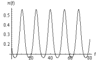
Figure 2: Number of reagents $n(t)=p(t)q(t)$ versus time $t$ obtained from numerically integrating dynamical system (37). The system is initialized with the conditions $p(0)=1/4$ and $q(0)=3/4$ which correspond to $n(0)=3/16$. The values of the parameters are $\mu=1$ and $\sigma=2$.

The fact that Hamiltonians like (36), which come from a chemical master equation, are not hermitian translates into the impossibility of expressing probabilities like (42) in terms of the physical variable $n$ rather than the formal auxiliary variables $p$ and $q$. Despite this undesirable fact, we can still characterize periodic orbits like the one represented in figure 2 by means of its period. Indeed, it is clear that for periodic solutions, the period of $p(t)$ and $q(t)$ will uniquely determine the period of $n(t)$. So a way to connect the physically measurable quantity $n$ with formula (42) is through the period of the oscillations of $n$. Of course, together with these large deviations, small fluctuations will be present all of the time. A way of distinguishing both of them is by means of their amplitude. The amplitude of small fluctuations is $O\left(\sqrt{\mu/\sigma}\right)$ while the amplitude of these oscillations promoted by large deviations is $O\left(\mu/\sigma\right)$. So the difference should certainly be measurable in the limit $\mu\gg\sigma$, which is exactly the range of validity of our WKB approximation.

3.2 Chemical chaos

Not only periodicity but also chaotic trajectories are possible in this simple system. To obtain them we allow the branching rate to be a periodic function of time $\mu\to\mu(t)>0$. Note that, due to the structure of system Eqs. (37), we could let either $\mu$, $\sigma$ or both be time dependent and still reduce the system to a $\mu$ time dependent one (while $\sigma$ remains constant) by means of a change of the temporal variable. In this case we deal with the system

$$\dot{p} = \mu(t)(p-p^{2})+\sigma(p^{2}-p)q,$$ (43)

$$\dot{q} = \mu(t)(2p-1)q+\frac{\sigma}{2}(1-2p)q^{2}.$$ (44)

Herein we still can identify three invariant lines: $\{p=0\}$, $\{p=1\}$ and $\{q=0\}$. The mean-field dynamics appears on the $\{p=1\}$ line, and is expressed by the equation

$$\dot{q}=\mu(t)q-\frac{\sigma}{2}q^{2}.$$ (45)

This differential equation is of Bernoulli type and can be solved to yield

$$q(t)=\frac{q(0)\exp\left[\int_{0}^{t}\mu(t_{1})dt_{1}\right]}{1+\frac{\sigma}{2}q(0)\int_{0}^{t}\exp\left[\int_{0}^{t_{1}}\mu(t_{2})dt_{2}\right]dt_{1}}.$$ (46)

Assuming that $\mu(t)=\mu+\epsilon h(t)$, where $h(t)$ is $T-$periodic and continuous and $\epsilon$ is a small enough constant, we know that there exists one $T-$periodic solution $q_{s}(t)$ which attracts all initial conditions $q(0)>0$. This is the solution whose initial condition fulfills

$$q(0)=\frac{\exp\left[\int_{0}^{T}\mu(t_{1})dt_{1}\right]-1}{\frac{\sigma}{2}\int_{0}^{T}\exp\left[\int_{0}^{t_{1}}\mu(t_{2})dt_{2}\right]dt_{1}}.$$ (47)

The points $(0,0)$ and $(1,0)$ continue to be fixed points in the non-autonomous system, and the point $(0,2\mu/\sigma)$ gives rise to a periodic orbit on $\{p=0\}$, which is formally identical to $q_{s}(t)$, but it is unstable on this line, and we will refer to it as $q_{u}(t)$. While the invariant line $\{q=2\mu/\sigma\}$ is not present in the perturbed system, the periodic trajectories $q_{s}(t)$ and $q_{u}(t)$ are still connected. They correspond to fixed points $\bar{q}_{s}$ and $\bar{q}_{u}$ of the Poincaré map associated to the forced continuous dynamical system. One may apply the theory developed in [27] to see that for generic perturbations $h(t)$ the unstable manifold of $\bar{q}_{s}$ intersects the stable manifold of $\bar{q}_{u}$ and thus guarantees the existence of a heteroclinic connection linking both fixed points.

The irregular behavior of the system dynamics comes from the fact that the periodic trajectories in the autonomous system may become quasiperiodic or even chaotic in the perturbed one. This can be justified by classical arguments from the Kolmogorov-Arnold-Moser (KAM) theory [28, 29] as follows.

Let us consider the stable equilibrium $P=(1/2,\mu/\sigma)$. The Floquet multipliers are by definition the eigenvalues of the corresponding Poincaré matrix. By the Hamiltonian structure, the Floquet multipliers are complex conjugate numbers $\lambda_{1},\lambda_{2}$ such that $\lambda_{1}\lambda_{2}=1$. For $P$, a direct computation on the linearized system gives $\lambda_{1}=e^{\omega iT}$, $\lambda_{2}=\overline{\lambda}_{1}$, with $\displaystyle{\omega=\mu/2}$. The equilibrium $P$ is said to be non-degenerate if $\displaystyle{\omega T\neq k\pi}$, for $k=1,\ldots,4$. A non-degenerate equilibrium is persistent under small perturbations as a fixed point of the Poincaré map. In other words, $P$ is continued as a $T$-periodic solution of the perturbed system (43)-(44) for small values of $\epsilon$. Besides, the presence of the heteroclinic loop corresponding to the energy level $H=0$ in the unperturbed system guarantees that the center around $P$ is not isochronous, that is, the Poincaré map is of twist type. Under such conditions, a generic perturbation gives rise to a classical KAM scenario, composed by a dense set of invariant tori (corresponding to quasiperiodic solutions) that are gradually destroyed as the perturbation increases, giving rise to domains of chaotic motion (Smale horseshoes) intermingled with stability islands.

Figure 3 shows a chaotic orbit surrounding a set of five stability islands. Such chaotic orbits arises from the destruction of an invariant torus that persists until a critical value of the perturbation parameter $\epsilon$. Figure 4 presents a zoom of the latter picture, where the typical fractal structure can be appreciated.

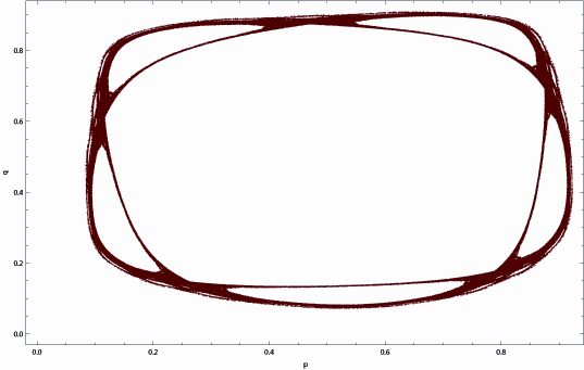
Figure 3: Numerical simulation showing chaos for system (43)-(44) with $h(t)=\sin{(2t)},\mu=1,\sigma=2,\epsilon=0.97$. It is drawn the Poincaré section of a single orbit with initial values $p(0)=0.53,q(0)=0.91$. More than $10^{5}$ points have been computed.

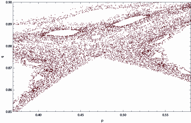
Figure 4: Zoom of Fig. 3. Besides the big stability islands, some smaller holes can be appreciated, conforming to a fractal structure.

Let us mention that the stability islands are centered in periodic orbits of higher periods (or subharmonic solutions). In the case of Figure 3, a subharmonic solution of order 5 is located at the stability islands. Section 5 is devoted to the study of the existence of such subharmonic solutions.

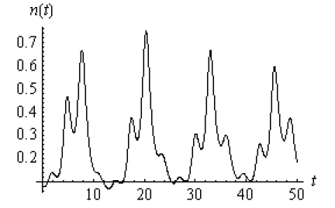
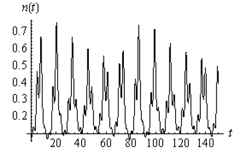
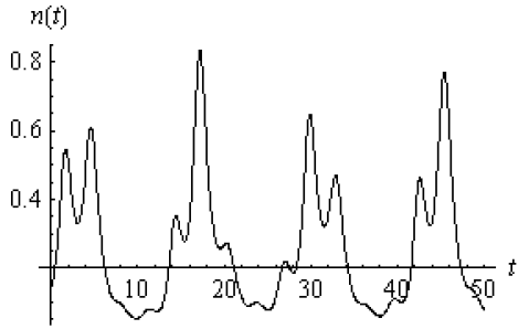
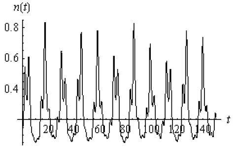
Figure 5: Number of reagents $n(t)=p(t)q(t)$ versus time $t$ obtained from numerically integrating dynamical system (43)-(44). The values of the parameters are $\mu=1$, $\sigma=2$ and $\epsilon=0.97$; the function $h(t)=\sin{(2t)}$. Panels 5 and 5: The system is initialized with the conditions $p(0)=1/5$ and $q(0)=2/5$ which correspond to $n(0)=2/25$. Panels 5 and 5: The system is initialized with the conditions $p(0)=3/5$ and $q(0)=1/4$ which correspond to $n(0)=3/20$.

We finish this section saying that we can compute the probability with which a chaotic orbit appears by means of the exponentiated negative of the action. This has already been done in explicitly time dependent chemical systems for the simpler extinction trajectories [30]. Herein we have shown that for exponentially long times the sort of Hamiltonian chaos we have described is possible for the simple reaction (31) by virtue of chemical noise. In absence of noise only periodic trajectories are possible. We have represented in figure 5 the resulting aperiodic trajectories for the number of reagents $n(t)=p(t)q(t)$ for two different time slots and initial conditions. Their physical interpretation is analogous to that of the periodic case in the last section. It is interesting to note that some of the irregular motions that can be observed in certain stochastic reaction dynamics might have an underlying deterministic structure (we are always referring to large deviations); let us recall that the time evolutions represented in figure 5 are purely deterministic.

4 Global continuation of the equilibrium point

In subsection 3.2 we point out that the equilibrium point $P=(1/2,\mu/\sigma)$ of system (37) is not degenerate if $\omega T\neq k\pi$, for $k=1,\dots,4$, with $\omega=\mu/2$. This property implies the continuation of $P$ as a $T$-periodic solution of the perturbed system (43)-(44) for small values of $\epsilon$. In this section we find an explicit interval $[0,E^{*}]$ for the parameter $\epsilon$ where this continuation exists and is unique. The main result is inspired by [31], where a similar technique is applied to the classical pendulum equation.

For simplicity in the calculations we apply the following change of variables to the perturbed system (43)-(44)

$$T:\mathbb{R}^{2}\to\mathbb{R}^{2},\quad T(p,q)=\Big{(}p-\frac{1}{2},q-\frac{\mu}{\sigma}\Big{)},$$ (48)

and obtain the new system

$$\left\{\begin{aligned} \dot{p}&=-\frac{\sigma}{4}q+\sigma p^{2}q+\epsilon\,h(t)(\frac{1}{4}-p^{2})\\ \dot{q}&=\frac{\mu^{2}}{\sigma}p-\sigma q^{2}p+2\epsilon h(t)(q+\frac{\mu}{\sigma})p\end{aligned}\right.$$ (49)

Note that for the perturbed system (49), the invariant lines are

$$\left\{p=-1/2\right\},\quad\left\{p=1/2\right\},\quad\left\{q=-\mu/\sigma\right\}.$$

In the following, we assume that $\displaystyle{\omega T/2\notin\mathbb{N}}$ with $\omega=\mu/2$.

Theorem 1.

. There exists $\beta=\beta(\omega,\sigma)$ such that for $\epsilon\in[0,E^{*}[$ with $\displaystyle{E^{*}=\frac{\sigma}{8\omega\beta h^{*}}}$, with $h^{*}=\max_{t\in[0,T]}\left\{h(t)\right\}$, system (49) has a unique non-trivial $T$-periodic solution $\Phi(t,\epsilon)=(\phi(t,\epsilon),\psi(t,\epsilon))$ as a continuation of the equilibrium point $P=(0,0)$ of the autonomous case.

Remark. From the proof, $\beta=\beta(\omega,\sigma)$ is explicitly given by

$$\beta=\beta(\omega,\sigma)=\displaystyle{\max_{t\in[0,T]}}\int_{0}^{T}|G(t,s)|ds,$$

where $G$ is a Green’s matrix function associated to the system (49) defined below, $|.|$ means the usual uniform matrix norm. The explicit bound

$$\beta(\omega,\sigma)<\frac{T}{|\sin(\omega T/2)|}\max\left\{\frac{1}{2},\frac{2}{\sigma},\frac{\sigma}{8\omega}\right\}.$$

is easily derived.

Proof.

We rewrite the system (49) in the form

$$\dot{X}=AX+B(t,X,\epsilon),$$ (50)

with

$$A=\begin{pmatrix}0&-\displaystyle{\sigma/4}\\ \displaystyle{\mu^{2}/\sigma}&0\end{pmatrix},\quad B(t,X,\epsilon)=\begin{pmatrix}B_{1}(t,X,\epsilon)\\ B_{2}(t,X,\epsilon)\end{pmatrix},$$

and

$$\begin{split}B_{1}(t,X,\epsilon)&=\displaystyle{\sigma p^{2}q+\epsilon\,h(t)(\frac{1}{4}-p^{2})},\\ B_{2}(t,X,\epsilon)&=-\sigma q^{2}p+2\epsilon\,h(t)(q+\frac{\mu}{\sigma})p.\end{split}$$

Now if $X(t,\epsilon)$ is a $T$-periodic solution of (50) the method of variation of constants provied us the next formula

$$X(t,\epsilon)=\int_{0}^{T}G(t,s)B(s,X(s,\epsilon),\epsilon)ds,$$ (51)

where $G(t,s)$ is the Green’s matrix function associated to this problem given by

$$G(t,s)=\begin{cases}\displaystyle{J^{-1}e^{(t-s)A}};&\textit{if}\quad 0\leq s\leq t\leq T\\ \displaystyle{J^{-1}e^{TA}e^{(t-s)A}};&\textit{if}\quad 0\leq t\leq s\leq T\end{cases}$$

where the matrix $J$ is defined by

$$J=(I_{2}-e^{TA})=\begin{pmatrix}\displaystyle{1-\cos\omega T}&\displaystyle{\frac{\sigma\omega}{4}\sin\omega T}\\ \displaystyle{-\frac{4\omega}{\sigma}\sin\omega T}&\displaystyle{1-\cos\omega T}\end{pmatrix}.$$

Explicitly, the Green’s matrix is

$$G(t,s)=\frac{1}{2}\begin{pmatrix}\displaystyle{\frac{\sin\omega(T/2-(t-s))}{\sin(\omega T/2)}}&-\displaystyle{\frac{\sigma}{4\omega}\frac{\cos\omega(T/2-(t-s))}{\sin(\omega T/2)}}\\ \displaystyle{\frac{4\omega}{\sigma}\frac{\cos\omega(T/2-(t-s))}{\sin(\omega T/2)}}&\displaystyle{\frac{\sin\omega(T/2-(t-s))}{\sin(\omega T/2)}}\end{pmatrix},$$

for all $0\leq s\leq t\leq T$ and

$$G(t,s)=\frac{1}{2}\begin{pmatrix}\displaystyle{\frac{\sin\omega((s-t)-T/2)}{\sin(\omega T/2)}}&-\displaystyle{\frac{\sigma}{4\omega}\frac{\cos\omega((s-t)-T/2)}{\sin(\omega T/2)}}\\ \displaystyle{\frac{4\omega}{\sigma}\frac{\cos\omega((s-t)-T/2)}{\sin(\omega T/2)}}&\displaystyle{\frac{\sin\omega((s-t)-T/2)}{\sin(\omega T/2)}}\end{pmatrix}$$

for $0\leq t\leq s\leq T$. In Appendix 1 we present the explicit calculation of (51).

Consider $\Omega=\mathbb{R}\times[0,E^{*}]$ and the normed space

$$E=\left\{X\in C(\Omega,\mathbb{R}^{2}):\textit{$X$ is $T$-periodic}\right\},$$

with the norm $\left\|\cdot\right\|_{\infty}$. We define the operator $\mathcal{T}:E\to E$ given by

$$(\mathcal{T}X)(t):=\int_{0}^{T}G(t,s)B(s,X(s,\epsilon),\epsilon)\,ds,$$

which is a completely continuous operator (with the norm $\left\|\cdot\right\|_{\infty}$ ) from $E$ to itself. It follows from (51) that $X(t,\epsilon)$ is a $T$-periodic solution of (50) if and only if $X$ is a fixed point of $\mathcal{T}$.

Now we concentrate on estimating a value $E^{*}$ where the operator $\mathcal{T}$ will be a contraction a let invariant a closed ball $\mathcal{B}=\left\{X\in E:\left\|X\right\|_{\infty}\leq\rho\right\}$ for some positive number $\rho=\rho(\omega,\sigma,\epsilon)$. To this end, let $X=(p,q)$, $Y=(\widetilde{p},\widetilde{q})$ inside the ball $\mathcal{B}$. Observe that

$$\begin{split}\left\|(\mathcal{T}X)(t)-(\mathcal{T}Y)(t)\right\|_{\infty}&=\left\|\int_{0}^{T}G(t,s)(B(s,X,\epsilon)-B(s,Y,\epsilon)ds\right\|_{\infty}\\ &\leq\Big{(}\displaystyle{\max_{t\in[0,T]}}\int_{0}^{T}|G(t,s)|ds\Big{)}\left\|B(s,X,\epsilon)-B(s,Y,\epsilon)\right\|_{\infty}\end{split}$$

where

$$\beta=\beta(\mu,\sigma)=\displaystyle{\max_{t\in[0,T]}}\int_{0}^{T}|G(t,s)|ds=\max_{1\leq i,j\leq 2}\Big{(}\max_{t\in[0,T]}\int_{0}^{T}|G_{i,j}(t,s)|ds\Big{)}.$$

Next we consider

$$B_{1}(t,X,\epsilon)-B_{1}(t,Y,\epsilon)=\displaystyle{\epsilon h(t)(\widetilde{p}^{2}-p^{2})+\sigma(p^{2}q-\widetilde{p}^{2}\widetilde{q})}.$$

Notes that

$$|\epsilon h(t)(\widetilde{p}^{2}-p^{2})|\leq 2\epsilon h^{*}\rho\left\|X-Y\right\|_{\infty},\quad\text{with}\quad h^{*}=\max_{t\in[0,T]}\left\{h(t)\right\},$$

and

$$|p^{2}q-\widetilde{p}^{2}\widetilde{q}|=|(p-\widetilde{p})(pq+\widetilde{p}q)+\widetilde{p}^{2}(q-\widetilde{q})|\leq 3\rho^{2}\left\|X-Y\right\|_{\infty}$$

therefore

$$\left\|B_{1}(t,X,\epsilon)-B_{1}(t,Y,\epsilon)\right\|_{\infty}\leq 2\rho(\epsilon h^{*}+3\sigma\rho/2)\left\|X-Y\right\|_{\infty}.$$

On the other hand

$$|B_{2}(t,X,\epsilon)-B_{2}(t,Y,\epsilon)|=|2\epsilon h(t)(qp-\widetilde{q}\widetilde{p})+\sigma(\widetilde{q}^{2}\widetilde{p}-q^{2}p)+\frac{2\epsilon h(t)\mu}{\sigma}(p-\widetilde{p})|.$$

For the first two terms in the right hand we have that

$$|\widetilde{q}^{2}\widetilde{p}-q^{2}p|=|(\widetilde{q}-q)(\widetilde{q}+p)p+\widetilde{q}^{2}\widetilde{p}-p\widetilde{q}|\leq 3\rho^{2}\left\|X-Y\right\|_{\infty},$$

and

$$|qp-\widetilde{q}\widetilde{p}|=|p(q-\widetilde{q})+(p-\widetilde{p})\widetilde{q}|\leq 2\rho\left\|X-Y\right\|_{\infty}$$

In consequence

$$\left\|B_{2}(t,X,\epsilon)-B_{2}(t,Y,\epsilon)\right\|_{\infty}\leq\Big{(}2\rho(\epsilon h^{*}+3\sigma\rho/2)+2\epsilon h^{*}(\rho+\mu/\sigma)\Big{)}\left\|X-Y\right\|_{\infty}$$

This estimate implies that

$$\left\|B(t,X,\epsilon)-B(t,Y,\epsilon)\right\|_{\infty}\leq\Big{(}2\rho(\epsilon h^{*}+3\sigma\rho/2)+2\epsilon h^{*}(\rho+\mu/\sigma)\Big{)}\left\|X-Y\right\|_{\infty}$$

Finally

$$\left\|\mathcal{T}X-\mathcal{T}Y\right\|_{\infty}\leq\beta\Big{(}2\rho(\epsilon h^{*}+3\sigma\rho/2)+2\epsilon h^{*}(\rho+\mu/\sigma)\Big{)}\left\|X-Y\right\|_{\infty}$$

From this last inequality, we concluded that the operator $\mathcal{T}$ will be a contraction if

$$\frac{3}{2}\sigma\rho^{2}+4\epsilon h^{*}\rho+\frac{2}{\sigma}\epsilon h^{*}\mu<\frac{1}{\beta}.$$

Now we use the fact that the quadratic convex function

$$f(\rho)=\frac{3}{2}\sigma\rho^{2}+4\epsilon h^{*}\rho+\frac{2}{\sigma}\epsilon h^{*}\mu-\frac{1}{\beta},$$

is negative in $[0,\rho_{0}[$ if $f(0)<0$, (this is equivalent to have $\displaystyle{\epsilon<\frac{\sigma}{4\mu\beta h^{*}}}$) with

$$\rho_{0}=\frac{-4\epsilon h^{*}+2\sqrt{\displaystyle{(2\epsilon h^{*})^{2}-3\sigma\Big{(}\frac{\epsilon\mu h^{*}}{\sigma}-\frac{1}{2\beta}\Big{)}}}}{3\sigma}.$$

In this way for $\epsilon\in[0,E^{*}[$ with $\displaystyle{E^{*}=\frac{\sigma}{4\mu\beta h^{*}}}$ we have

$$\left\|\mathcal{T}X-\mathcal{T}Y\right\|_{\infty}\leq k\left\|X-Y\right\|_{\infty}$$

with $0<k<1$ for all $X,Y\in\mathcal{B}$. Remains to knows the size of radius of the ball $\mathcal{B}$. Let $Y_{0}=(0,0)$, then

$$(\mathcal{T}Y_{0})(t)=\frac{\epsilon}{4}\begin{pmatrix}\displaystyle{\int_{0}^{T}G_{1,1}(t,s)h(s)ds}\\ \displaystyle{\int_{0}^{T}G_{2,1}(t,s)h(s)ds}\end{pmatrix},$$

moreover

$$\left\|\mathcal{T}X\right\|_{\infty}-\left\|\mathcal{T}Y_{0}\right\|_{\infty}\leq\left\|\mathcal{T}X-\mathcal{T}Y_{0}\right\|_{\infty}\leq k\left\|X-Y_{0}\right\|_{\infty}$$

this implies

$$\left\|\mathcal{T}X\right\|_{\infty}\leq k\left\|X\right\|_{\infty}+\left\|\mathcal{T}Y_{0}\right\|_{\infty}=k\rho+\epsilon h^{*}\beta/4.$$

We take $\displaystyle{\rho=\frac{\epsilon h^{*}\beta}{4(1-k)}}$ and $\epsilon$ small enough sucht that $f(\rho)<0$. Combining these estimatives we have that

$$\left\|\mathcal{T}X\right\|_{\infty}\leq\rho,\quad\text{and}\quad\left\|\mathcal{T}X-\mathcal{T}Y\right\|_{\infty}<k\left\|X-Y\right\|_{\infty},$$

for all $X,Y\in\mathcal{B}.$ Then $\mathcal{T}$ maps the closed ball $\mathcal{B}$ into itself. Thus it follows from the Schauder fixed point theorem [33] that $\mathcal{T}$ has a fixed point $\Phi$ in $\mathcal{B}$. Since $\mathcal{T}:\mathcal{B}\to\mathcal{B}$ is a contraction then $\mathcal{T}$ the fixed point is unique. ∎

5 Local continuation of periodic solutions from the autonomous case

From Section 3 we know that $P=(1/2,\mu/\sigma)$ is an equilibrium point for the autonomous system (37). Moreover $P$ is a center and therefore there is a domain of periodic solutions around $P$. In Section 4, after a change of coordinates (48), the point $P$ is extended for $\epsilon\in\,]0,E^{*}]$ as a $T$-periodic solution $\Phi(t,\epsilon)$ of (49). Furthermore, this extension is unique and continuous.

In this section, we look for multiplicity of periodic solutions. To this purpose, we assume that $h(t)$ is an even function. Under this assumption, (49) has the following symmetry

$$(t,p,q)\to(-t,-p,q).$$

Our aim is to obtain $nT$-periodic solutions of (49) as a result of the local continuation of $nT$-periodic solutions of the autonomous Hamiltonian system (37). To this end we present the next result which is inspired by the results on [32, Section 5].

Some notation is needed. $[\cdot]$ denotes the integer part function. Fix $n_{*}=\displaystyle{\big{[}\frac{2\pi}{\omega\,T}]}$. For a fixed integer $n\geq n_{*}$, define $\displaystyle{\vartheta_{n}=\big{[}\frac{\omega\,nT}{2\pi}]}$.

Theorem 2.

For all $n>n_{*}$ and $m=1,\dots,\vartheta_{n}$, there exists $\epsilon_{n,m}>0$ such that for all $0<\epsilon<\epsilon_{n,m}$ system (49) has a non-trivial $nT$-periodic solution $X(t,\epsilon)=(p(t,\epsilon),q(t,\epsilon))$ where $q(t,\epsilon)$ crosses exactly $m$ times through the horizontal line $q=0$ in the interval $[0,nT/2]$.

Proof.

Let $X(t;\xi,0)=(p(t;\xi,0),q(t,\xi,0))$ a solution (49) in the autonomous case ($\epsilon=0$) satisfying the initial condition

$$p(0,\xi,0)=0,\quad q(0,\xi,0)=\xi,$$ (52)

and the boundary condition

$$p(nT/2,\xi,0)=0.$$ (53)

In Appendix 2 we prove that the family of periodic solutions $X(t;\xi,0)$ of (49) for $0<\xi<\mu/\sigma$ has an increasing period function $T(\xi)$ such that

$$\lim_{\xi\searrow 0}T(\xi)=T_{lp}\quad\text{and}\quad\lim_{\xi\nearrow\mu/\sigma}T(\xi)=\infty,$$

with $\displaystyle{T_{lp}=2\pi/\omega}$. Moreover, in the autonomous case we have the following symmetry

$$(t,p,q)\to(-t,p,-q),$$

therefore we can assume that $\xi>0$. Given $n\in\mathbb{N}$, $X(t;\xi,0)$ is a $nT$-periodic solution of (49) if and only if there is an integer $m\geq 1$ such that

$$m\,T(\xi)=nT.$$ (54)

Since

$$\inf T(\xi)=T_{lp}=\frac{2\pi}{\omega},$$

we have $\displaystyle{\frac{nT}{m}>\frac{2\pi}{\omega}}$ therefore $\displaystyle{m<\frac{\omega\,nT}{2\pi}}$.

Let

$$\mu/\sigma>\xi_{1}>\xi_{2}>\dots>\xi_{\vartheta_{n}}>0,$$

be the solutions of (54) with $m=1,2,\dots,\vartheta_{n}$. Since we consider the boundary condition (53) Then

$$\begin{split}\mathcal{K}_{0}&=\left\{\xi\in\mathbb{R}:p(nT/2,\xi,0)=0\right\}\\ &=\{-\xi_{1},\dots,-\xi_{\vartheta_{N}},\,0\,,\xi_{1},\dots,\xi_{\vartheta_{N}}\}.\\ \end{split}$$

Now we compute the index for $\xi_{1}\in\mathcal{K}_{0}$. Note the following

• If $\xi<\xi_{1}$ then $\displaystyle{\frac{T(\xi)}{2}<\frac{T(\xi_{1})}{2}=nT/2},$

• If $\xi>\xi_{1}$ then $\displaystyle{\frac{T(\xi)}{2}>\frac{T(\xi_{1})}{2}=nT/2}.$

Since $T(\xi)$ is increasing, we have for values $\xi$ close to $\xi_{1}$ that

$$\begin{split}p(nT/2;\xi,0)>0&\quad\text{if}\quad\xi<\xi_{1},\\ p(nT/2;\xi,0)<0&\quad\text{if}\quad\xi>\xi_{1}.\end{split}$$

From here, the Brouwer index $\text{ind}(p(nT/2,\cdot,0),\xi_{1})=-1$ (see for instance [34] for definition and basic properties). From the previous calculus we can conclude that in general

$$\text{ind}((p(nT/2,\cdot,0),\xi_{m})=(-1)^{m}.$$ (55)

By symmetry the indices of $-\xi_{m}$ are $\text{ind}(p(nT/2,\cdot,0),\xi_{m})=(-1)^{m+1}$. We also calculate the index at $\xi_{0}=0$. We do this by linearization, i.e.,

$$\text{ind}((p(nT/2,\cdot,0),0)=\text{sign}\Big{(}\frac{\partial p}{\partial\xi}(nT/2;0,0)\Big{)}.$$

To this end we consider the linearized problem of at $(0,\xi)$ and we observe that $\displaystyle{\frac{\partial X}{\partial\xi}(t,\xi,0)}$ is solution of the initial value problem

$$\dot{X}=AX,\quad X(0)=\begin{pmatrix}0\\ 1\end{pmatrix},$$

therefore

$$\text{ind}((p(nT/2,\cdot,0),0)=\text{sign}\Big{(}\frac{4\omega}{\sigma}\sin\big{(}\frac{\omega\,nT}{2}\big{)}\Big{)}=(-1)^{\vartheta_{n}}.$$

In conclusion for $\epsilon=0$ there exists $\vartheta_{n}$ nontrivial $nT$-periodic solutions of (62) with

$$p(0;\xi,0)=0,\quad q(0;\xi,0)=\xi>0,$$

such solutions can be labeled according to the number of times $m$ that the function $\displaystyle{q(t;\xi,0)}$ passes through the horizontal line $q=0$ in $[0,nT/2]$ with $m=1,\ldots,\vartheta_{n}$ and initial conditions

$$\mu/\sigma>q_{1}(0)=\xi_{1}>\cdots>q_{\vartheta_{n}}(0)=\xi_{\vartheta_{n}}>0.$$

From (55) and the Implicit Function theorem, for each $n\geq n_{*}$ with $\displaystyle{n_{*}=[\frac{2\pi}{\omega T}]}$ the is a $C^{1}$ function $E:[0,\epsilon_{n,m}[\to\mathbb{R}$, $\epsilon\to E(\epsilon)$ such that $X(t,\epsilon)$ is a $nT$-periodic solution of (49) that satisfy the initial condition

$$X(0,\epsilon)=\begin{pmatrix}0\\ E(\epsilon)\end{pmatrix},$$

and the boundary condition

$$p(nT/2,E(\epsilon),\epsilon)=0,$$

for all $\epsilon\in[0,\epsilon_{n,m}[.$ This completes the proof.

∎

6 Conclusions and outlook

In this work we have shown the appearance of chaotic and periodic behavior in chemical systems as a direct consequence of internal fluctuations. We have concentrated on the simple reaction $A\longleftrightarrow 2A$, which at the mean-field (fluctuations free) level simply shows logistic growth. While this theory correctly predicts the short time behavior, long times are dominated by fluctuations. In this case we have seen that fluctuations may sustain metastable states and periodic orbits. For this same reaction, if we allow the reaction rates to vary periodically in time we find the presence of chaotic orbits sustained by chemical noise, while the mean-field theory only reflects periodic orbits. We have also been able to rigorously prove the existence of even and periodic solutions of the nonautonomous system as a result of the global continuation of even and periodic solutions of the autonomous system. It is important to remark here that the deterministic trajectories studied here will not be observed in experiments, but their noisy counterparts. That is, small Gaussian distributed fluctuations about the deterministic trajectories studied herein will be present at any time. We also note that the appearance of periodicity and chaos in chemical reactions due to intrinsic fluctuations has already been investigated [35, 36, 37]. Nevertheless our approach is fundamentally different as these previous studies focused on systems close to a bifurcation threshold. So the periodic and chaotic behaviors were already present in the mean-field deterministic dynamics, and the internal noise anticipated the threshold. In our case, the mean-field dynamics were of too low dimensionality for showing periodic and chaotic orbits respectively. In this sense, the oscillations and chaos were purely sustained by chemical fluctuations.

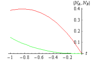
Figure 6: Optimal paths to extinction in Lotka-Volterra dynamics (57) for $\mu=\sigma=\lambda=1$. The initial numbers of predators (represented by the red upper line) and preys (represented by the green lower line) are respectively $N_{A}(t=-1)\approx 0.39$ and $N_{B}(t=-1)\approx 0.15$. The extinction takes place at $t=0$ and for $p_{a}=p_{b}=0$, $q_{a}=-1$ and $q_{b}=1$. The trajectories lie in $H=1$ manifold.

We have also studied the optimal paths to extinction in a plankton population dynamics model. Although extinction phenomena have been considered numerous times within this framework [13, 14, 30], the approach was based on the Hamiltonian dynamics on the stationary $H=0$ manifold. The Hamiltonian dynamical system in our case was however degenerated and all the extinction trajectories fell on the $H\neq 0$ manifolds. We leave for future work the extension of our results to multispecies reactions, which are characterized by large deviation Hamiltonian dynamical systems of higher dimension. Notably, there is an important problem of a two species reaction which is very much related to the plankton extinction described herein. It is the appearance of extinction events in the predator-prey Lotka-Volterra dynamics. This dynamics is formalized by means of the reaction set

$$A\stackrel{{\scriptstyle\mu}}{{\longrightarrow}}\emptyset,\quad B\stackrel{{\scriptstyle\sigma}}{{\longrightarrow}}2B,\quad A+B\stackrel{{\scriptstyle\lambda}}{{\longrightarrow}}2A,$$ (56)

where $A$ is the predator and $B$ is the prey. This system has been studied by means of a diffusion approximation and solving the corresponding Fokker-Planck equation [38]. A different alternative is using a large deviations approach, which yields the Hamiltonian

$$\mathcal{H}=\mu(p_{a}-1)q_{a}-\sigma p_{b}(p_{b}-1)q_{b}+\lambda p_{a}(p_{b}-p_{a})q_{a}q_{b}.$$ (57)

The numbers of predator and prey are given respectively by $N_{A}(t)=p_{a}(t)q_{a}(t)$ and $N_{B}(t)=p_{b}(t)q_{b}(t)$. The optimal paths to extinction appear again on $H\neq 0$ manifolds. We have numerically computed two of them in Fig. 6. A large deviation drives the system to extinction which takes place when $p_{a}$ and $p_{b}$ become zero. One can see in this figure that the decreasing number of preys pulls the predators to extinction, as it is reasonable to expect. Alternatively, a large deviation driving the predators to extinction will lead to an unbounded growth of the preys. We expect that a systematic study of the extinction trajectories of the Lotka-Volterra Hamiltonian (57) will shed a valuable light on the probabilistic structure of extinction events in predator-prey dynamics.

Appendix 1

The purpose of this appendix is to show more explicitly the calculations to obtain the expression of the operator $\mathcal{T}$ in the formula (51). To this end, consider the system

$$\dot{X}=AX+B(t,X)$$ (58)

with

$$A=\begin{pmatrix}0&-\displaystyle{\sigma/4}\\ \displaystyle{\mu^{2}/\sigma}&0\end{pmatrix},\quad B(t,X)=\begin{pmatrix}B_{1}(t,X)\\ B_{2}(t,X)\end{pmatrix},$$

The fundamental matrix of the associated autonomous system $\dot{X}=AX$ is the exponential matrix $e^{tA}$ given by

$$e^{tA}=\begin{pmatrix}\cos\omega t&-\displaystyle{\frac{\sigma}{4\omega}}\sin\omega t\\ \displaystyle{\frac{4\omega}{\sigma}}\sin\omega t&\cos\omega t\end{pmatrix}.$$

Then by the method of variations of constants the general solution of $(\ref{As})$ is given by

$$\begin{split}X(t)=e^{tA}C+\int_{0}^{t}e^{(t-s)A}B(s,X)\,ds,\end{split}$$ (59)

where $C$ a constant vector. Since we are looking for $T$-periodic solutions imposing the boundary conditions $X(0)=X(T)$ we get

$$C=e^{TA}C+\int_{0}^{T}e^{(t-s)A}B(s,X)\,ds$$

this implies

$$\begin{split}(I_{2}-e^{TA})C&=\int_{0}^{T}e^{(T-s)A}B(s,X)\,ds\\ C&=(I_{2}-e^{TA})^{-1}\int_{0}^{T}e^{(T-s)A}B(s,X)\,ds,\end{split}$$

replacing this in the formula $(\ref{As-2})$ we obtain

$$X(t)=e^{tA}(I_{2}-e^{TA})^{-1}\int_{0}^{T}e^{(T-s)A}B(s,X)\,ds+\int_{0}^{t}e^{(t-s)A}B(s,X)\,ds,$$

On the other hand

$$J=(I_{2}-e^{TA})=\begin{pmatrix}1-\cos\omega T&\displaystyle{\frac{\sigma}{4\omega}}\sin\omega T\\ -\displaystyle{\frac{4\omega}{\sigma}}\sin\omega T&1-\cos\omega T\end{pmatrix},$$

since $\det{J}=2(1-\cos\omega T)$ then

$$J^{-1}=\frac{1}{2}\begin{pmatrix}1&-\displaystyle{\frac{\sigma}{4\omega}}\frac{\cos(\omega T/2)}{\sin(\omega T/2)}\\ \displaystyle{\frac{4\omega}{\sigma}}\frac{\cos(\omega T/2)}{\sin(\omega T/2)}&1\end{pmatrix},$$

by direct calculation it is found that

$$e^{tA}J^{-1}=J^{-1}e^{tA},\qquad e^{tA}e^{(T-s)A}=e^{TA}e^{(t-s)A}.$$

Therefore

$$\begin{split}X(t)&=J^{-1}e^{TA}\int_{0}^{T}e^{(T-s)A}B(s,X)\,ds+\int_{0}^{t}e^{(t-s)A}B(s,X)\,ds\\ X(t)&=[J^{-1}e^{TA}+I_{2}]\int_{0}^{t}e^{(t-s)A}B(s,X)\,ds+J^{-1}e^{TA}\int_{t}^{T}e^{(t-s)A}B(s,X)\,ds\end{split}$$

The matrix $J$ satisfies $J^{-1}=J^{-1}e^{TA}+I_{2}$. In consequence

$$X(t)=J^{-1}\int_{0}^{t}e^{(t-s)A}B(s,X)\,ds+J^{-1}e^{TA}\int_{t}^{T}e^{(t-s)A}B(s,X)\,ds$$

We define the Green’s matrix

$$G(t,s)=\begin{cases}\displaystyle{J^{-1}e^{(t-s)A}};&\textit{if}\quad 0\leq s\leq t\leq T\\ \displaystyle{J^{-1}e^{TA}e^{(t-s)A}};&\textit{if}\quad 0\leq t\leq s\leq T\end{cases}$$

Thus we can write

$$X(t)=\int_{0}^{t}G(t,s)B(s,X)\,ds$$

Let $G_{1}=J^{-1}e^{(t-s)A}$. Explicitly this matrix is given by

$$G_{1}=\begin{pmatrix}\frac{\cos\omega(t-s)\sin(\omega T/2)-\cos(\omega T/2)\sin\omega(t-s)}{2\sin(\omega T/2)}&-\frac{\sigma}{4\omega}[\frac{\sin\omega(t-s)\sin(\omega T/2)+\cos(\omega T/2)\cos\omega(t-s)}{2\sin(\omega T/2)}]\\ \frac{4\omega}{\sigma}[\frac{\cos\omega(t-s)\cos(\omega T/2)-\sin(\omega T/2)\sin\omega(t-s)}{2\sin(\omega T/2)}]&\frac{\cos\omega(t-s)\sin(\omega T/2)-\cos(\omega T/2)\sin\omega(t-s)}{2\sin(\omega T/2)}\end{pmatrix}$$

From the trigonometric identities follows easily

$$J^{-1}e^{(t-s)A}=\frac{1}{2}\begin{pmatrix}\displaystyle{\frac{\sin\omega(T/2-(t-s))}{\sin(\omega T/2)}}&-\displaystyle{\frac{\sigma}{4\omega}\frac{\cos\omega(T/2-(t-s))}{\sin(\omega T/2)}}\\ \displaystyle{\frac{4\omega}{\sigma}\frac{\cos\omega(T/2-(t-s))}{\sin(\omega T/2)}}&\displaystyle{\frac{\sin\omega(T/2-(t-s))}{\sin(\omega T/2)}}\end{pmatrix},$$

Let $G_{2}=J^{-1}e^{TA}e^{(t-s)A}$. Explicitly this matrix is given by

$$G_{2}=\begin{pmatrix}-\frac{1}{2}&-\frac{\sigma}{4\omega}\frac{\cos(\omega T/2)}{2\sin(\omega T/2)}\\ \frac{4\omega}{\sigma}\frac{\cos(\omega T/2)}{2\sin(\omega T/2)}&-\frac{1}{2}\end{pmatrix}\begin{pmatrix}\cos\omega(t-s)&-\frac{\sigma}{4\omega}\sin\omega(t-s)\\ \frac{4\omega}{\sigma}\sin\omega(t-s)&\cos\omega(t-s)\end{pmatrix}.$$

By direct calculation

$$G_{2}=\begin{pmatrix}\frac{-\cos\omega(t-s)\sin(\omega T/2)-\cos(\omega T/2)\sin\omega(t-s)}{2\sin(\omega T/2)}&-\frac{\sigma}{4\omega}[\frac{\cos(\omega T/2)\cos\omega(t-s)-\sin\omega(t-s)\sin(\omega T/2)}{2\sin(\omega T/2)}]\\ \frac{4\omega}{\sigma}[\frac{\cos(\omega T/2)\cos\omega(t-s)-\sin\omega(t-s)\sin(\omega T/2)}{2\sin(\omega T/2)}]&\frac{-\cos\omega(t-s)\sin(\omega T/2)-\cos(\omega T/2)\sin\omega(t-s)}{2\sin(\omega T/2)}\end{pmatrix},$$

again, using basic trigonometric identities follows that

$$J^{-1}e^{TA}e^{(t-s)A}=\frac{1}{2}\begin{pmatrix}\displaystyle{\frac{\sin\omega((s-t)-T/2)}{\sin(\omega T/2)}}&-\displaystyle{\frac{\sigma}{4\omega}\frac{\cos\omega((s-t)-T/2)}{\sin(\omega T/2)}}\\ \displaystyle{\frac{4\omega}{\sigma}\frac{\cos\omega((s-t)-T/2)}{\sin(\omega T/2)}}&\displaystyle{\frac{\sin\omega((s-t)-T/2)}{\sin(\omega T/2)}}\end{pmatrix}.$$

In orther to present a upper bound for the constant $\beta(\omega,\sigma)$ we give the calculations for

$$\max_{t\in[0,T]}\int_{0}^{T}|G_{1,1}(t,s)|ds$$

To this end, observe that

$$\int_{0}^{T}|G_{1,1}(t,s)|ds=\frac{1}{2}\Big{[}\int_{0}^{t}\Big{|}\frac{\sin\omega(T/2-(t-s))}{\sin(\omega T/2)}\Big{|}\,ds+\int_{t}^{T}\Big{|}\frac{\sin\omega(T/2-(s-t))}{\sin(\omega T/2)}\Big{|}\,ds\Big{]}.$$

On the other hand

$$\frac{1}{2}\int_{0}^{t}\Big{|}\frac{\sin\omega(T/2-(t-s))}{\sin(\omega T/2)}\Big{|}\,ds=\frac{1}{2\omega}\int_{\omega(T/2-t)}^{\omega T/2}\Big{|}\frac{\sin u}{\sin(\omega T/2)}\Big{|}\,du,$$

and also

$$\int_{t}^{T}\Big{|}\frac{\sin\omega(T/2-(s-t))}{\sin(\omega T/2)}\Big{|}\,ds=-\frac{1}{2\omega}\int_{\omega T/2}^{\omega(t-T/2)}\Big{|}\frac{\sin u}{\sin(\omega T/2)}\Big{|}\,du.$$

It follows that

$$\int_{0}^{T}|G_{1,1}(t,s)|ds=\frac{1}{\omega}\int_{0}^{\omega T/2}\frac{|\sin u|}{|\sin(\omega T/2)|}\,ds$$

The same analysis applies to other components of the matrix $G$ and we obtain

$$\begin{split}\int_{0}^{T}|G_{1,2}(t,s)|ds&=\frac{\sigma}{4\omega^{2}}\int_{0}^{\omega T/2}\frac{|\cos u|}{|\sin(\omega T/2)|}\,ds,\\ \int_{0}^{T}|G_{2,1}(t,s)|ds&=\frac{4}{\sigma}\int_{0}^{\omega T/2}\frac{|\cos u|}{|\sin(\omega T/2)|}\,ds,\\ \int_{0}^{T}|G_{2,2}(t,s)|ds&=\frac{1}{\omega}\int_{0}^{\omega T/2}\frac{|\sin u|}{|\sin(\omega T/2)|}\,ds.\end{split}$$

Since

$$\beta=\beta(\mu,\sigma)=\displaystyle{\max_{t\in[0,T]}}\int_{0}^{T}|G(t,s)|ds=\max_{1\leq i,j\leq 2}\Big{(}\max_{t\in[0,T]}\int_{0}^{T}|G_{i,j}(t,s)|ds\Big{)},$$

follows that

$$\beta(\omega,\sigma)<\frac{T}{|\sin\omega T/2|}\max\left\{\frac{1}{2},\frac{2}{\sigma},\frac{\sigma}{8\omega}\right\}.$$

Appendix 2

In this appendix we are going to study the period function of periodic solutions around the center $(1/2,\mu/\sigma)$ for the autonomous case. Given the clear symmetry of the vector field of our Hamiltonian system (37) around the center we consider the next change of variables

$$T:\mathbb{R}^{2}\rightarrow\mathbb{R}^{2},\quad T(p,q)=\bigg{(}p-\frac{1}{2},q-\frac{\mu}{\sigma}\bigg{)}.$$ (60)

We obtain in the new coordinates $(\overline{p},\overline{q})$ the quadratic Hamiltonian function

$$\mathcal{H}(\overline{p},\overline{q})=-\frac{\sigma}{2}\bigg{(}\overline{p}^{2}-\frac{1}{4}\bigg{)}\bigg{(}\overline{q}^{2}-\frac{\mu^{2}}{\sigma^{2}}\bigg{)}.$$ (61)

$\mathcal{H}(\overline{p},\overline{q})$ has the following symmetries

$$\begin{split}\text{S}_{1}&:(\overline{p},\overline{q})\rightarrow(\overline{p},-\overline{q}),\\ \text{S}_{2}&:(\overline{p},\overline{q})\rightarrow(-\overline{p},-\overline{q}),\\ \text{S}_{3}&:(\overline{p},\overline{q})\rightarrow(-\overline{p},\overline{q}).\end{split}$$

The corresponding dynamical system is

$$\left\{\begin{aligned} \dot{\overline{p}}&=-\frac{\sigma}{4}\overline{q}+\sigma\overline{q}\,\overline{p}^{2}\\ \dot{\overline{q}}&=\frac{\mu^{2}}{\sigma}\overline{p}-\sigma\overline{p}\,\overline{q}^{2}\end{aligned}\right.$$ (62)

The invariant lines are now

$$\left\{\overline{p}=-1/2\right\},\quad\left\{\overline{p}=1/2\right\},\quad\left\{\overline{q}=-\mu/\sigma\right\}\quad\text{and}\quad\left\{\overline{q}=\mu/\sigma\right\}.$$

They define a new quadrangular area $\mathcal{A}$ which center is our equilibrium point $(0,0)$. See Fig. 7.

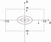
Figure 7: Quadrangular region $\mathcal{A}$.

Consider a periodic solution $\overline{X}(t)=(\overline{p}(t),\overline{q}(t))$ of (62) inside $\mathcal{A}$ with initial conditions

$$\overline{p}(0)=\zeta,\quad\overline{q}(0)=0,$$ (63)

this implies that $\zeta$ satisfies $-1/2<\zeta<1/2$. Since $\mathcal{H}$ is a first integral of (62) we take the level set

$$h=\mathcal{H}(\zeta,0)=\frac{\mu^{2}}{2\sigma}(\zeta^{2}-\frac{1}{4}),$$

and consider the equation

$$\begin{split}\mathcal{H}(\overline{p}(t),\overline{q}(t))&=h\\ -\frac{\sigma}{2}\big{(}\overline{p}^{2}(t)-\frac{1}{4}\big{)}\big{(}\overline{q}^{2}(t)-\frac{\mu^{2}}{\sigma^{2}}\big{)}&=\frac{\mu^{2}}{2\sigma}(\zeta^{2}-\frac{1}{4}),\\ \end{split}$$

which can be written as

$$-(4\overline{p}^{2}(t)-1)(\sigma^{2}\overline{q}^{2}(t)-\mu^{2})=\mu^{2}(4\zeta^{2}-1).$$

By the symmetry $\text{S}_{2}$ we can take $0<\overline{p}^{2}(t)<\zeta^{2}<1/4$ and get from direct calculus

$$\sigma^{2}\overline{q}^{2}(t)=\frac{4\mu^{2}(\overline{p}^{2}(t)-\zeta^{2})}{4\overline{p}^{2}(t)-1}.$$

From (62) it follows that

$$\overline{q}=\frac{\dot{\overline{p}}}{\sigma(\overline{p}^{2}-\frac{1}{4})},$$

and we finally have

$$\dot{\overline{p}}^{2}(t)=\frac{1}{4}\mu^{2}(\overline{p}^{2}(t)-\zeta^{2})(4\overline{p}^{2}(t)-1).$$

Note that the right hand side in the last equation is positive. Let $T(\zeta)$ be the period of the solution $\overline{X}(t)$ of (62) satisfying (63). We have

$$\begin{split}\int_{0}^{T(\zeta)/4}dt&=\int_{0}^{T(\zeta)/4}\frac{-1}{\sqrt{\frac{1}{4}\mu^{2}(\overline{p}^{2}-\zeta^{2})(4\overline{p}^{2}-1)}}\frac{d\overline{p}}{dt}\,dt,\\ T(\zeta)&=\frac{8}{\mu}\int_{0}^{\zeta}\frac{1}{\sqrt{(\overline{p}^{2}-\zeta^{2})(4\overline{p}^{2}-1)}}d\overline{p}.\end{split}$$

If $\overline{p}=\zeta v$, then

$$T(\zeta)=\frac{8}{\mu}K(2\zeta),$$

where $\displaystyle{K(x)=\int_{0}^{1}\frac{1}{\sqrt{(1-v^{2})(1-x^{2}v^{2})}}dv}$ is the complete elliptic integral of the first kind. On the other hand the linearized problem of (62) about the equilibrium solution $(0,0)$ is given by

$$\left\{\begin{aligned} \dot{y}_{1}&=-\frac{\sigma}{4}\,y_{2}\\ \dot{y}_{2}&=\frac{\mu^{2}}{\sigma}\,y_{1}\end{aligned}\right.$$

and its general solution is

$$\begin{split}y_{1}&=-C_{1}\frac{\sigma}{2\mu}\sin\Big{(}\frac{\mu}{2}t\Big{)}+C_{2}\cos\Big{(}\frac{\mu}{2}t\Big{)},\\ y_{2}&=C_{1}\cos\Big{(}\frac{\mu}{2}t\Big{)}+\frac{2\mu}{\sigma}C_{2}\sin\Big{(}\frac{\mu}{2}t\Big{)},\end{split}$$

This shows that the period of the linear problem is $\displaystyle{T_{lp}=\frac{4\pi}{\mu}}.$

From the above discussions we are now in position to prove the next statement.

Proposition 1.

Let $\overline{X}(t;\zeta)=(\overline{p}(t;\zeta),\overline{q}(t;\zeta))$ be a non trivial periodic solution of (62) that satisfies the initial conditions (63). If $T(\zeta)$ is the period function of $\overline{X}(t;\zeta)$ this function satisfies the following properties

(a)

$\displaystyle\lim_{\zeta\to 0^{+}}T(\zeta)=T_{lp}.$

(b)

$\displaystyle\lim_{\zeta\rightarrow\frac{1}{2}^{-}}T(\zeta)=\infty.$

(c)

$\displaystyle{\frac{dT}{d\zeta}>0}$ for all $0<\zeta<\frac{1}{2}.$

Proof. The proof of $(a)$ and $(b)$ follows from the well know properties of the complete elliptic integral of the first kind function. Moreover

$$K(2\xi)=\int_{0}^{1}\frac{1}{\sqrt{(1-v^{2})(1-4\xi^{2}v^{2})}}dv=\int_{0}^{\pi/2}\frac{1}{\sqrt{1-4\xi^{2}\sin^{2}\theta}}d\theta.$$

To prove (c) consider the real function

$$f(\theta,\zeta)=\frac{1}{\sqrt{1-4\xi^{2}\sin^{2}\theta}},$$

with $f:[0,\pi/2]\times[0,1/2[\to\mathbb{R}$. This function satisfies

• $f(\cdotp,\zeta)$ is a Riemann integrable function in $[0,\pi/2]$, for all $\zeta\in[0,1/2[$,

• $f(\theta,\cdotp)$ is a differentiable function in $[0,1/2[$, for all $\theta\in[0,\pi/2]$,

furthermore $\displaystyle{\frac{\partial f}{\partial\zeta}}$ is continuous in $[0,\pi/2]\times[0,1/2[$. The previous observations over the function $f$ are the hypothesis of the classic version of the rule of derivation under the integral, then

$$\frac{dT}{d\zeta}=\frac{4\zeta}{\mu}\int_{0}^{\pi/2}\frac{\sin^{2}\theta}{(1-4\zeta^{2}\sin^{2}\theta)^{3/2}}d\theta>0,$$

and this proves (c). $\square$

Observation. By symmetry of the system (62) , the above proposition is also true if we consider non trivial solutions $\overline{X}(t;\eta)=(\overline{p}(t;\eta),\overline{q}(t;\eta))$ that satisfies the initial conditions

$$\overline{p}(0)=0,\quad\overline{q}(0)=\eta,$$

with $0<\eta<\mu/\sigma$.

References

- [1] N. G. van Kampen, Stochastic Processes in Physics and Chemistry (Noth-Holland, Amsterdam, 2001).
- [2] C. W. Gardiner, Handbook of Stochastic Methods (Springer, Berlin, 2004).
- [3] R. Kubo, K. Matsuo, and K. Kitahara, J. Stat. Phys. 9, 51 (1973).
- [4] B. J. Matkowsky, Z. Schuss, C. Knessl, C. Tier, and M. Mangel, Phys. Rev. A 29, 3359 (1984).
- [5] C. Knessl, B. J. Matkowsky, Z. Schuss, and C. Tier, SIAM J. Appl. Math. 45, 1006 (1985).
- [6] M. M. Klosek-Dygas, B. J. Matkowsky, and Z. Schuss, SIAM J. Appl. Math. 49, 1811 (1989).
- [7] M. I. Dykman, E. Mori, J. Ross, and P. M. Hunt, J. Chem. Phys. 100, 5735 (1994).
- [8] M. I. Dykman, T. Horita, and J. Ross, J. Chem. Phys. 103, 966 (1995).
- [9] V. Elgart and A. Kamenev, Phys. Rev. E 70, 041106 (2004).
- [10] C. R. Doering, K. V. Sargsyan, and L. M. Sander, Multi-scale Model. and Simul. 3, 283 (2005).
- [11] V. Elgart and A. Kamenev, Phys. Rev. E 74, 041101 (2006).
- [12] C. R. Doering, K. V. Sargsyan, L. M. Sander, and E. Vanden-Eijnden, J. Phys.: Condens. Matter 19, 065145 (2007).
- [13] M. Assaf and B. Meerson, Phys. Rev. Lett. 97, 200602 (2006).
- [14] M. Assaf and B. Meerson, Phys. Rev. E 75, 031122 (2007).
- [15] C. Escudero and A. Kamenev, Phys. Rev. E 79, 041149 (2009).
- [16] H. Treutlein and K. Schulten, Ber. Bunsenges. Phys. Chem. 89, 710 (1985).
- [17] J. R. Pradines, G. V. Osipov, and J. J. Collins, Phys. Rev. E 60, 6407 (1999).
- [18] B. Lindner, J. García-Ojalvo, A. Neiman, and L. Schimansky-Geier, Phys. Rep. 392, 321 (2004).
- [19] W. Liebermeister, J. Theor. Biol. 234, 423 (2005).
- [20] K. L. Davis and M. R. Roussel, FEBS J. 27, 84 (2006).
- [21] B. Øksendal, Stochastic Differential Equations. An Introduction with Applications, (Springer-Verlag, Berlin, 2003).
- [22] M. I. Freidlin and A. D. Wentzell, Random perturbations of dynamical systems, (Springer-Verlag, New York, 1998).
- [23] Y.-C. Zhang, M. Serva, and M. Polikarpov, J. Stat. Phys. 58, 849 (1990).
- [24] R. Adler, Monte Carlo simulation in oceanography, Proceedings of the 10th ’Aha Huliko’a Hawaiian Winter Workshop, University of Hawaii at Manoa (1997).
- [25] W. R. Young, A. J. Roberts, and G. Stuhne, Nature (London) 412, 328 (2001).
- [26] F. Baumann, M. Henkel, M. Pleimling, and J. Richert, J. Phys. A: Math. Gen. 38, 6623 (2005).
- [27] C. Escudero and J. Á. Rodríguez, Phys. Rev. E 77, 011130 (2008).
- [28] V. Arnold, Méthodes Mathematiques de la Mechanique Classique, MIR, Moscow, 1976.
- [29] C. Siegel, M. Moser, Lectures on Celestial Mechanics, Springer-Verlag, Berlin, 1971.
- [30] M. Assaf, A. Kamenev, and B. Meerson, Phys. Rev. E 78, 041123 (2008).
- [31] J. Lei, X. Li, P. Yan and M. Zhang, Twist character of the least amplitude periodic solution of the forced pendulum, SIAM J. Math. Anal. 35 (2003), 844–867.
- [32] J. Llibre and R. Ortega, On the families of periodic orbits of the Sitnikov problem, SIAM J. Applied Dynamical Systems, 7 (2008) 561-576.
- [33] J. Leray and J. Schauder, Topologie et équations fontionnelles, Ann. Sci. École Norm. Sup. (3), 51 (1934), pp. 45-78.
- [34] K. Deimling, Nonlinear Functional analysis, Springer-Verlag, Berlin, 1985.
- [35] X.-G. Wu and R. Kapral, Phys. Rev. Lett. 70, 1940 (1993).
- [36] X.-G. Wu and R. Kapral, Phys. Rev. E 50, 3560 (1994).
- [37] W. Vance and J. Ross, J. Chem. Phys. 105, 479 (1996).
- [38] M. Parker and A. Kamenev, Phys. Rev. E 80, 021129 (2009).