Model-independent determination of sharp features inside a star from its oscillation frequencies

Abstract

It has been established earlier that sharp features like the base of the convective zone or the second helium ionisation zone inside a star give rise to sinusoidal oscillations in the frequencies of pulsation. The acoustic depth of such features can be estimated from this oscillatory signal in the frequencies. We apply this technique for the CoRoT frequencies of the solar-type star HD 49933. This is the first time that such analysis has been done of seismic data for any star other than the Sun. We are able to determine the acoustic depth of both the base of the convective zone and the HeII ionisation zone of HD 49933 within $10\%$ error from the second differences of the frequencies. The locations of these layers using this technique is in agreement with the current seismic models of HD 49933.

1 Introduction

A discontinuity in the derivatives of the sound speed in the stellar interior introduces a characteristic oscillatory signature in the frequencies of low degree modes of the form (Gough 1990)

$$\sin(4\pi\nu\tau+\phi)$$

where $\tau$ is the acoustic depth of the layer, lying at a radius $r$, given by

$$\tau=\int_{r}^{R}\mathrm{d}r/c$$

and $\nu$ is the frequency of oscillation. $\phi$ is a phase factor.

In solar-type stars, the base of the convective envelope and the HeII ionisation zones are the most prominent layers of such discontinuity. Each of these layers contributes to a sinusoidal variation in the frequencies of pulsation with the periodicity corresponding to the respective acoustic depth of the layer. The resulting combined signal in the frequencies can be fitted to a suitable functional form to extract the acoustic depths of these layers separately. Here we apply this technique to estimate the acoustic depths of these regions of the solar-type star HD 49933 from its frequencies obtained from the CoRoT satellite (Baglin et al. 2006). Although this method has been used with great success for the Sun (see e.g., Basu et al. 1994; Monteiro et al. 1994), this is the first instance of an application to a distant star. This was one of the main objectives of the CoRoT seismology programme (Michel et al. 2006).

The significance of this method is that it does not depend on theoretical stellar models – the position of the sharp features are estimated directly from the frequencies themselves. In fact, such independent determination of these layers can help in the modelling of the star, as illustrated by Mazumdar (2005). We describe the technique used in this work and the results in the next two sections.

2 Technique

This oscillatory signal in the frequencies is quite small and is embedded in the frequencies together with a smooth variation of the frequencies arising from the regular variation of the sound speed in the stellar interior. It can be enhanced by using the second differences (see, e.g., Basu et al. 1994; Mazumdar & Antia 2001; Basu et al. 2004),

$$\delta^{2}\nu(n,\ell)=\nu(n-1,\ell)-2\nu(n,\ell)+\nu(n+1,\ell),$$ (1)

instead of the frequencies themselves. Using the second differences serves the dual purpose of removing the smooth component in frequencies, and magnifying the oscillatory components. However, the errors in the frequencies are also enhanced in taking the differences, which might obscure the oscillatory signal. This is the reason why one cannot use even higher differences.

The acoustic depths of the base of the convective zone (BCZ) and the second helium ionisation zone (HIZ), $\tau_{\mathrm{\scriptscriptstyle BCZ}}$ and $\tau_{\mathrm{\scriptscriptstyle HIZ}}$, respectively, can be obtained from the data by fitting the second differences to a suitable function representing the oscillatory signals from these layers (Mazumdar & Antia 2001). We choose the following function along the lines of Basu et al. (2004):

$$\delta^{2}\nu = a_{0}+b_{0}\sin(4\pi\nu\tau_{\mathrm{\scriptscriptstyle BCZ}}\!+\!\phi_{\mathrm{\scriptscriptstyle BCZ}})$$ (2)

$$+(c_{0}\!+\!c_{1}/\nu)\sin(4\pi\nu\tau_{\mathrm{\scriptscriptstyle HIZ}}\!+\!\phi_{\mathrm{\scriptscriptstyle HIZ}})$$

This function has three components corresponding to a residual smooth variation, and the two oscillatory components corresponding to BCZ and HIZ. We do not use all the parameters in the function suggested by Basu et al. (2004) to accurately represent the second differences because one cannot afford to use too many free parameters for a relatively small data set. The number of free parameters is optimised to strike a balance between a fair representation of the oscillatory signal and a reasonable $\chi^{2}$. We find that the smooth component is fairly constant over the range of frequencies that we use, as is the amplitude of the signal from the BCZ. However, the amplitude of the signal from the HIZ varies more sharply with frequency, and thus requires at least one frequency-dependent term. We note that Basu et al. (2004) have shown that the exact form of the amplitudes of the oscillatory signal does not affect the results significantly.

The fit is carried out through a nonlinear $\chi^{2}$ minimisation, weighted by the errors in the data. The errors in the second differences are correlated, and this is taken care of by defining the $\chi^{2}$ using a covariance matrix. The contribution of the errors are considered by producing $1000$ realisations of the data, where the mean values of the frequencies are skewed by random errors corresponding to a normal distribution. The successful convergence of such a non-linear fitting procedure is somewhat dependent on the choice of reasonable initial guesses. To remove the effect of initial guesses affecting the final fitted parameters, we carry out the fit for multiple combinations of starting values. For each realisation, $100$ combinations of initial guesses are tried for fitting the function above and the one with the minimum $\chi^{2}$ is accepted as the fit for that particular realisation.

The median value of each parameter for its distribution over $1000$ realisations is taken as the average. The error in the parameter is estimated from the range of values covering $68\%$ area about the median (corresponding to $1\sigma$ error). As an example, the histogram of distribution of the parameters $\tau_{\mathrm{\scriptscriptstyle BCZ}}$ and $\tau_{\mathrm{\scriptscriptstyle HIZ}}$ over $1000$ realisations are illustrated in Figs. 2 and 3. The quoted errors in these parameters reflect the width of these histograms on two sides of the median value.

3 Results

Our primary data set is that of Benomar et al. (2009). To check for consistency we also use the data set of Gruberbauer et al. (2009), and the theoretical frequencies of a model of HD 49933 (Deheuvels 2010; see also Goupil 2010).

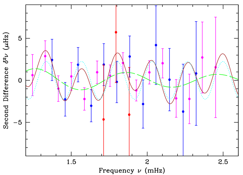
Figure 1: Second differences of frequencies of HD 49933 from $180$ days of CoRoT data (Benomar et al. 2009) are plotted against frequencies for $\ell=0$ (blue points), $\ell=1$ (magenta points), and a few $\ell=2$ (red points) modes. The fit of the oscillatory function is shown by the brown solid line. The cyan dotted line shows the fitted oscillatory signal due to the base of the convection zone (BCZ) and the green dashed line shows the signal due to the second helium ionisation zone (HIZ)

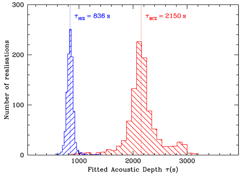
Figure 2: Histograms of fitted values of acoustic depths, $\tau_{\mathrm{\scriptscriptstyle BCZ}}$ (red) and $\tau_{\mathrm{\scriptscriptstyle HIZ}}$ (blue), obtained for $1000$ different realisations of the data according to Benomar et al. (2009) are shown. The median values are shown with the dotted lines.

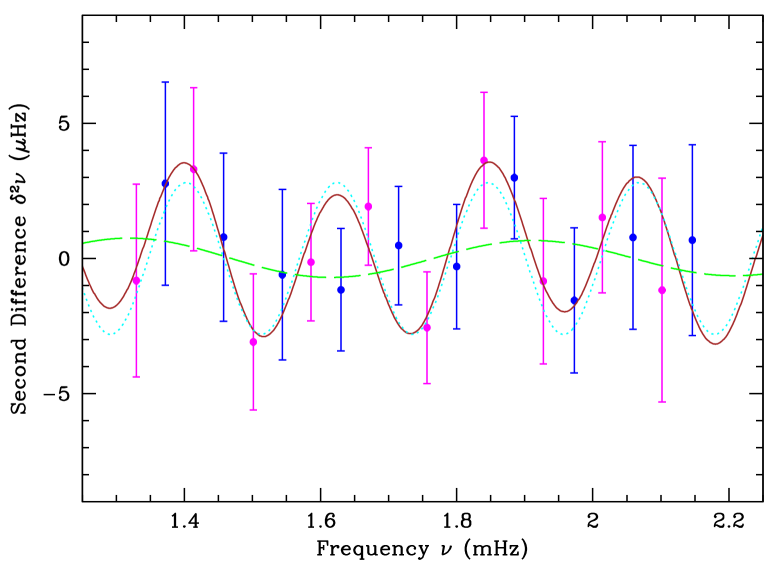
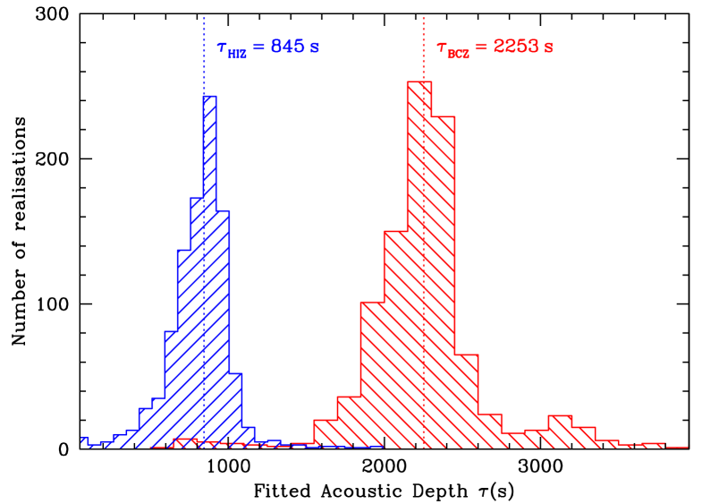
Figure 3: Similar plots as Figs. 1 and 2, but with the frequencies taken from the 60 day CoRoT data (Gruberbauer et al. 2009).

The fit of the function given in Eq. 2 is shown in Fig. 1 for the data set from Benomar et al. (2009). This set consists of $31$ second differences computed from the individual frequencies. We did not use frequencies which had errors of more than $3\,\mu\mathrm{Hz}$. The data represented in this figure corresponds to the mean frequencies. In reality, different realisations of the data are fitted independently. The figure also shows the function given in Eq. 2, with the parameter values set equal to the median values obtained from $1000$ realisations. The histograms of $\tau_{\mathrm{\scriptscriptstyle BCZ}}$ and $\tau_{\mathrm{\scriptscriptstyle HIZ}}$ values over all realisations are shown in Fig. 2. The median values are indicated, and the errors are estimated by considering the extent of the histogram around the median such that $34\%$ of the cases are covered on each side. Since the histograms are asymmetric, naturally this yields unequal error bars. We consider these to be representative of $1\sigma$ error on the median value of the parameter concerned. The average amplitude of the oscillatory components corresponding to the two regions, $A_{\mathrm{\scriptscriptstyle BCZ}}$ and $A_{\mathrm{\scriptscriptstyle HIZ}}$, are evaluated in terms of the frequencies themselves, instead of the second differences (see Mazumdar & Antia 2001, for details). These results are summarised in Table 1.

To check for consistency, we also used the data set from Gruberbauer et al. (2009), which yielded $20$ second differences. This data set yields very similar results, shown in Fig. 3 and listed in Table 1, although with higher error bars, showing that the method works even with lesser data.

Lastly, we also fit Eq. 2 to the theoretical frequencies computed from a stellar model of HD 49933 (Deheuvels 2010; Goupil 2010). The actual model values of the acoustic depths, $\tau_{\mathrm{\scriptscriptstyle BCZ}}$ and $\tau_{\mathrm{\scriptscriptstyle HIZ}}$, are remarkably close to the values obtained from this fit (see Table 1). This is not entirely unexpected, since the stellar model is obtained by matching the seismic frequencies themselves. However, the methods used in the seismic modelling do not explicitly involve determining the depths of the base of the convective envelope or the second helium ionisation region. In contrast, our method focuses directly on these two layers, irrespective of the stratification in the rest of the star. However, as pointed out by Mazumdar (2005), the location of these layers cannot be independent of the structure of the rest of the star, and is thus linked implicitly to the detailed model. But the process of fitting the acoustic depths does not involve stellar modelling and thus the results obtained in this method are completely model-independent.

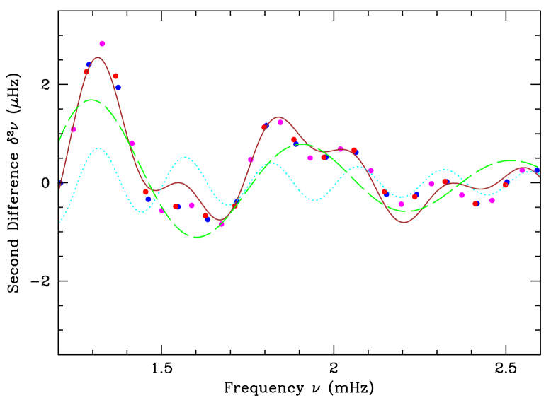
Figure 4: Second differences of frequencies of a theoretical model of HD 49933 (Deheuvels 2010; Goupil 2010) are plotted against frequencies for $\ell=0$, $\ell=1$, and $\ell=2$ modes. The composite fit of the the oscillatory function, as well as its two components are shown, similar to Fig. 1.

Table 1: Results of the fitting of second differences to Eq. 2 for two data sets and a theoretical model. The quantities in parentheses represent the errors in each parameter for the first two rows, and the actual theoretical model values in the third row.

Data Set	No. of	Acoustic Depth		Average Amplitude in $\nu$		$\chi^{2}$
	data pts.	$\tau_{\mathrm{\scriptscriptstyle BCZ}}$ (s)	$\tau_{\mathrm{\scriptscriptstyle HIZ}}$ (s)	$A_{\mathrm{\scriptscriptstyle BCZ}}$($\mu\mathrm{Hz}$)	$A_{\mathrm{\scriptscriptstyle HIZ}}$($\mu\mathrm{Hz}$)
CoRoT $180$ d (Benomar et al. 2009)	$31$	$2150$ ($+182$/$-257$)	$836$ ($+56$/$-52$)	$0.57$ ($\pm 0.30$)	$1.29$ ($\pm 0.30$)	$1.03$
CoRoT $60$ d (Gruberbauer et al. 2009)	$20$	$2253$ ($+289$/$-226$)	$845$ ($+191$/$-142$)	$0.52$ ($\pm 0.20$)	$0.93$ ($\pm 0.32$)	$0.83$
Model (Deheuvels 2010; Goupil 2010)	$57$	$1995$ ($1999$)	$826$ ($883$)	$0.46$	$1.35$

4 Summary

We have determined the acoustic positions of the base of the convective envelope and the second helium ionisation zone in the star HD 49933 from the oscillatory signal in its frequencies observed with CoRoT. The method involves fitting a suitable function to represent the two oscillatory signals arising from the two zones to the second differences of the frequencies. We find almost similar results for two data sets, one corresponding to only the initial 60-day run of CoRoT and another a 180-day combined time-series obtained with a long run of CoRoT. This is the first instance where such a technique has been successfully applied to a star other than the Sun.

Although these results are independent of any stellar modelling, they match well with a seismic model of the star. In fact the acoustic depths of such layers of sharp changes in the sound speed inside the star extracted in this method can help to model the star (Mazumdar 2005).

The same technique can be used to estimate the acoustic depths of such layers in other stars. We have established that a time series of moderate length, as obtained by CoRoT, is sufficient for the successful application of this technique. A longer time series, as expected from the Kepler mission, for example, would further reduce the errors on the extracted acoustic depths.