Sloan Low-mass Wide Pairs of Kinematically Equivalent Stars (SLoWPoKES):
A Catalog of Very Wide, Low-mass Pairs

Abstract

We present the Sloan Low-mass Wide Pairs of Kinematically Equivalent Stars (SLoWPoKES), a catalog of 1342 very-wide (projected separation $\gtrsim 500$ AU), low-mass (at least one mid-K – mid-M dwarf component) common proper motion pairs identified from astrometry, photometry, and proper motions in the Sloan Digital Sky Survey. A Monte Carlo based Galactic model is constructed to assess the probability of chance alignment for each pair; only pairs with a probability of chance alignment $\leq 0.05$ are included in the catalog. The overall fidelity of the catalog is expected to be 98.35%. The selection algorithm is purposely exclusive to ensure that the resulting catalog is efficient for follow-up studies of low-mass pairs. The SLoWPoKES catalog is the largest sample of wide, low-mass pairs to date and is intended as an ongoing community resource for detailed study of bona fide systems. Here we summarize the general characteristics of the SLoWPoKES sample and present preliminary results describing the properties of wide, low-mass pairs. While the majority of the identified pairs are disk dwarfs, there are 70 halo subdwarf pairs and 21 white dwarf–disk dwarf pairs, as well as four triples. Most SLoWPoKES pairs violate the previously defined empirical limits for maximum angular separation or binding energies. However, they are well within the theoretical limits and should prove very useful in putting firm constraints on the maximum size of binary systems and on different formation scenarios. We find a lower limit to the wide binary frequency for the mid-K – mid-M spectral types that constitute our sample to be 1.1%. This frequency decreases as a function of Galactic height, indicating a time evolution of the wide binary frequency. In addition, the semi-major axes of the SLoWPoKES systems exhibit a distinctly bimodal distribution, with a break at separations around 0.1 pc that is also manifested in the system binding energy. Comparing with theoretical predictions for the disruption of binary systems with time, we conclude that the SLoWPoKES sample comprises two populations of wide binaries: an “old” population of tightly bound systems, and a “young” population of weakly bound systems that will not survive more than a few Gyr. The SLoWPoKES catalog and future ancillary data are publicly available on the world wide web for utilization by the astronomy community.

1. Introduction

The formation and evolution of binary stars remains one of the key unanswered questions in stellar astronomy. As most stars are thought to form in multiple systems, and with the possibility that binaries may host exoplanet systems, these questions are of even more importance. While accurate measurements of the fundamental properties of binary systems provide constraints on evolutionary models (e.g. Stassun et al., 2007), knowing the binary frequency, as well as the distribution of the periods, separations, mass ratios, and eccentricities of a large ensemble of binary systems are critical to understanding binary formation (Goodwin et al., 2007, and references therein). To date, multiplicity has been most extensively studied for the relatively bright high- and solar-mass local field populations (e.g. Duquennoy & Mayor, 1991, hereafter DM91). Similar studies of low-mass M and L dwarfs have been limited by the lack of statistically significant samples due to their intrinsic faintness. However, M dwarfs constitute $\sim$70% of Milky Way’s stellar population (Miller & Scalo, 1979; Henry et al., 1999; Reid et al., 2002; Bochanski et al., 2010, hereafter B10) and significantly influence its properties.

Since the pioneering study of Heintz (1969), binarity has been observed to decrease as a function of mass: the fraction of primaries with companions drops from 75% for OB stars in clusters (Gies, 1987; Mason et al., 1998, 2009) to $\sim$60% for solar-mass stars (Abt & Levy 1976, DM91, Halbwachs et al. 2003) to $\sim$30–40% for M dwarfs (Fischer & Marcy 1992, hereafter FM92; Henry & McCarthy 1993; Reid & Gizis 1997; Delfosse et al. 2004) to $\sim$15% for brown dwarfs (BDs; Bouy et al., 2003; Close et al., 2003; Gizis et al., 2003; Martín et al., 2003). This decrease in binarity with mass is probably a result of preferential destruction of lower binding energy systems over time by dynamical interactions with other stars and molecular clouds, rather than a true representation of the multiplicity at birth (Goodwin & Kroupa, 2005). In addition to having a smaller total mass, lower-mass stars have longer main-sequence (MS) lifetimes (Laughlin, Bodenheimer, & Adams, 1997) and, as an ensemble, have lived longer and been more affected by dynamical interactions. Hence, they are more susceptible to disruption over their lifetime. Studies of young stellar populations (e.g. in Taurus, Ophiucus, Chameleon) appear to support this argument, as their multiplicity is twice as high as that in the field (Leinert et al., 1993; Ghez et al., 1997; Kohler & Leinert, 1998). However, in denser star-forming regions in the Orion Nebula Cluster and IC 348, where more dynamical interactions are expected, the multiplicity is comparable to the field (Simon, Close, & Beck 1999; Petr et al. 1998; Duchêne, Bouvier, & Simon 1999). Hence, preferential destruction is likely to play an important role in the evolution of binary systems.

DM91 found that the physical separation of the binaries could be described by a log-normal distribution, with the peak at $a\sim$30 AU and $\sigma_{\log a}\sim$1.5 for F and G dwarfs in the local neighborhood. The M dwarfs in the local 20-pc sample of FM92 seem to follow a similar distribution with a peak at $a\sim$3–30 AU, a result severely limited by the small number of binaries in the sample.

Importantly, both of these results suggest the existence of very wide systems, separated in some cases by more than a parsec. Among the nearby ($d<$ 100 pc) solar-type stars in the Hipparcos catalog, Lépine & Bongiorno (2007) found that 9.5% have companions with projected orbital separations $s>$ 1000 AU. However, we do not have a firm handle on the widest binary that can be formed or on how they are affected by localized Galactic potentials as they traverse the Galaxy. Hence, a sample of wide binaries, especially one that spans a large range of heliocentric distances, would help in (i) putting empirical constraints on the widest binary systems in the field (e.g. Reid et al., 2001a; Burgasser et al., 2003, 2007; Close et al., 2003, 2007), (ii) understanding the evolution of wide binaries over time (e.g., Weinberg, Shapiro, & Wasserman, 1987; Jiang & Tremaine, 2009), and (iii) tracing the inhomogeneities in the Galactic potential (e.g. Bahcall, Hut, & Tremaine 1985 Weinberg et al. 1987; Yoo, Chanamé, & Gould 2004; Quinn et al. 2009).

Recent large scale surveys, such as the Sloan Digital Sky Survey (SDSS; York et al., 2000), the Two Micron All Sky Survey (2MASS; Cutri et al., 2003), and the UKIRT Infrared Deep Sky Survey (UKIDSS; Lawrence et al., 2007), have yielded samples of unprecedented numbers of low-mass stars. SDSS alone has a photometric catalog of more than 30 million low-mass dwarfs (B10), defined as mid-K – late-M dwarfs for the rest of the paper and a spectroscopic catalog of more than 44000 M dwarfs (West et al., 2008). The large astrometric and photometric catalogs of low-mass stars afford us the opportunity to explore anew the binary properties of the most numerous constituents of Milky Way, particularly at the very widest binary separations.

The orbital periods of very wide binaries (orbital separation $a>$ 100  AU) are much longer than the human timescale ($P=$ 1000 yr for  M_tot$=$ 1 M_⊙ and $a=$ 100 AU). Thus, these systems can only be identified astrometrically, accompanied by proper motion or radial velocity matching. These also remain some of the most under-explored low-mass systems. Without the benefit of retracing the binary orbit, two methods have been historically used to identify very wide pairs:

1. Bahcall & Soneira (1981) used the two-point correlation method to argue that the excess of pairs found at small separations is a signature of physically associated pairs; binarity of some of these systems was later confirmed by radial velocity observations (Latham et al., 1984). See Garnavich (1988) and Wasserman & Weinberg (1991) for other studies that use this method.

2. To reduce the number of false positives inherent in the above, one can use additional information such as proper motions. Orbital motions for wide systems are small; hence, the space velocities of a gravitationally bound pair should be the same, within some uncertainty. In the absence of radial velocities, which are very hard to obtain for a very large number of field stars, proper motion alone can be used to identify binary systems; the resulting pairs are known as common proper-motion (CPM) doubles. Luyten (1979, 1988) pioneered this technique in his surveys of Schmidt telescope plates using a blink microscope and detected more than 6000 wide CPM doubles with $\mu>$100 mas yr^-1 over almost fifty years. This method has since been used to find CPM doubles in the AGK 3 stars by Halbwachs (1986), in the revised New Luyten Two-Tenths (rNLTT; Salim & Gould, 2003) catalog by Chanamé & Gould (2004), and among the Hipparcos stars in the Lepine-Shara Proper Motion-North (LSPM-N; Lépine & Shara, 2005) catalog by Lépine & Bongiorno (2007). All of these studies use magnitude-limited high proper-motion catalogs and, thus, select mostly nearby stars.

More recently, Sesar, Ivezić, & Jurić (2008, hereafter SIJ08) searched the SDSS Data Release Six (DR6; Adelman-McCarthy et al., 2008) for CPM binaries with angular separations up to 30$\arcsec$ using a novel statistical technique that minimizes the difference between the distance moduli obtained from photometric parallax relations for candidate pairs. They matched proper motion components to within 5 mas yr^-1 and identified $\sim$22000 total candidates with excellent completeness, but with a one-third of them expected to be false positives. They searched the SDSS DR6 catalog for pairs at all mass ranges and find pairs separated by 2000–47000 AU, at distances up to 4 kpc. Similarly, Longhitano & Binggeli (2010) used the angular two-point correlation function to do a purely statistical study of wide binaries in the $\sim$675 square degrees centered at the North Galactic Pole using the DR6 stellar catalog and predicted that there are more than 800 binaries with physical separations larger than 0.1 pc but smaller than 0.8 pc. As evidenced by the large false positive rate in SIJ08, such large-scale searches for wide binaries generally involve a trade-off between completeness on the one hand and fidelity on the other, as they depend on statistical arguments for identification.

Complementing this type of ensemble approach, a high-fidelity approach may suffer from incompleteness and/or biases; however, there are a number of advantages to a “pure” sample of bona fide wide binaries such as that presented in this work. For example, Faherty et al. (2010) searched for CPM companions around the brown dwarfs in the BDKP catalog (Faherty et al., 2009) and found nine nearby pairs; all of their pairs were followed up spectroscopically and, hence, have a much higher probability of being real. As mass, age, and metallicity can all cause variations in the observed physical properties, e.g. in radius or in magnetic activity, their effects can be very hard to disentangle in a study of single stars. Components of multiple systems are expected to have been formed of the same material at the same time, within a few hundred thousand years of each other (e.g. White & Ghez 2001; Goodwin, Whitworth, & Ward-Thompson 2004; Stassun et al. 2008). Hence, binaries are perfect tools for separating the effects of mass, age, and metallicity from each other as well as for constraining theoretical models of stellar evolution. Some examples include benchmarking stellar evolutionary tracks (e.g. White et al. 1999; Stassun, Mathieu, & Valenti 2007; Stassun et al. 2008), investigating the age-activity relations of M dwarfs (e.g. Silvestri, Hawley, & Oswalt, 2005), defining the dwarf-subdwarf boundary for spectral classification (e.g. Lépine et al., 2007), and calibrating the metallicity indices (Woolf & Wallerstein, 2005; Bonfils et al., 2005). Moreover, equal-mass multiples can be selected to provide identical twins with the same initial conditions (same mass, age, and metallicity) to explore the intrinsic variations of stellar properties. In addition, wide binaries (a $>$ 100 AU) are expected to evolve independently of each other; even their disks are unaffected by the distant companion (Clarke, 1992). Components of such systems are effectively two single stars that share their formation and evolutionary history. In essence they can be looked at as coeval laboratories that can be used to effectively test and calibrate relations measured for field stars. Finally, as interest has grown in detecting exoplanets and in characterizing the variety of stellar environments in which they form and evolve, a large sample of bona fide wide binaries could provide a rich exoplanet hunting ground for future missions such as SIM.

In this paper, we present a new catalog of CPM doubles from SDSS, each with at least one low-mass component, identified by matching proper motions and photometric distances. In § 2 we describe the origin of the input sample of low-mass stars; § 3 details the binary selection algorithm and the construction of a Galactic model built to assess the fidelity of each binary in our sample. The resulting catalog and its characteristics are discussed in § 4. We compare the result of our CPM double search with previous studies in § 5 and summarize our conclusions in § 6.

2. SDSS Data

2.1. SDSS Sample of Low-Mass Stars

SDSS is a comprehensive imaging and spectroscopic survey of the northern sky using five broad optical bands ($ugriz$) between $\sim$3000–10000Å using a dedicated 2.5 m telescope (York et al., 2000; Fukugita et al., 1996; Gunn et al., 1998). Data Release Seven (DR7; Abazajian et al., 2009) contains photometry of 357 million unique objects over 11663 $\deg^{2}$ of the sky and spectra of over 1.6 million objects over 9380 $\deg^{2}$ of the sky. The photometry has calibration errors of 2% in $u$ and $\sim$1% in $griz$, with completeness limits of 95% down to magnitudes 22.0, 22.2, 22.2, 21.3, 20.5 and saturation at magnitudes 12.0, 14.1, 14.1, 13.8, 12.3, respectively (Gunn et al., 1998). We restricted our sample to $r\leq 20$ where the SDSS/USNO-B proper motions are more reliable (see § 2.3); hence, photometric quality and completeness should be excellent for our sample.

Stellar sources with angular separations $\gtrsim$ 0.5–0.7$\arcsec$ are resolved in SDSS photometry; we determined this empirically from a search in the Neighbors table. For sources brighter than $r\sim$ 20, the astrometric accuracy is 45 mas rms per coordinate while the relative astrometry between filters is accurate to 25–35 mas rms (Pier et al., 2003).

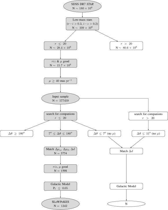
Figure 1.— A graphical representation of the selection process used in the identification of SLoWPoKES pairs. The gray boxes show the steps involved in SLoWPoKES, with the results presented in this paper. The pairs without proper motions (shown in white boxes) will be presented in a follow-up paper.

The SDSS DR7 photometric database has more than 180 million stellar sources (Abazajian et al., 2009); to select a sample of low-mass stars, we followed the procedures outlined in B10 and required $r-i\geq$ 0.3 and $i-z\geq$ 0.2, which represents the locus of sample K5 or later dwarfs. The star table was used to ensure that all of the selected objects had morphology consistent with being point sources (type $=$ 6) and were not duplicate detections of the same source (primary). This yielded a sample of $>$ 109 million low-mass stars with $r\sim$ 14–24, at distances of $\sim$0.01–5 kpc from the Sun. Figure 1 shows a graphical flow chart of the selection process and criteria used; the steps needed in identifying kinematic companions, which are detailed in this paper, are shown in gray boxes. The white boxes show subsets where kinematic information is not available; however, it is still possible to identify binary companions based on their close proximity. We will discuss the selection of binaries, without available kinematic information, in a future paper.

2.2. Proper Motions

The SDSS/USNO-B matched catalog (Munn et al., 2004), which is integrated into the SDSS database in the ProperMotions table, was used to obtain proper motions for this study. We used the proper motions from the DR7 catalog; the earlier data releases had a systematic error in the calculation of proper motion in right ascension (see Munn et al., 2008, for details). This catalog uses SDSS galaxies to recalibrate the USNO-B positions and USNO-B stellar astrometry as an additional epoch for improved proper motion measurements. The ProperMotions catalog is resolution limited in the USNO-B observations to 7$\arcsec$ and is 90% complete to $g=$ 19.7, corresponding to the faintness limit of the POSS-II plates used in USNO-B. The completeness also drops with increasing proper motion; for the range of proper motions in our sample ($\mu=$ 40–350 mas yr^-1; see § 2.3 below), the completeness is $\sim$ 85%. The typical 1 $\sigma$ error is 2.5–5 mas yr^-1 for each component

2.3. Quality Cuts

To ensure that the resultant sample of binaries is not contaminated due to bad or suspect data, we made a series of cuts on the stellar photometry and proper motions. With $>$ 109 million low-mass stars, we could afford to be very conservative in our quality cuts and still have a reasonable number of stars in our input sample. We restricted our sample, as shown in Figure 1, to stars brighter than $r=$ 20 and made a cut on the standard quality flags on the $riz$ magnitudes (peakcenter, notchecked, psf_flux_interp, interp_center, bad_counts_error, saturated – all of which are required to be 0), which are the only bands pertinent to low-mass stars and the only bands used in our analysis.

On the proper motions, Munn et al. (2004) recommended a minimum total proper motion of 20 mas yr^-1 and cuts based on different flags for a “clean” and reliable sample of stellar sources. Therefore, we required that each star (i) matched an unique USNO-B source within 1$\arcsec$ (match $>$ 0), (ii) had no other SDSS source brighter than $g=$ 22 within 7$\arcsec$ (dist22 $>$ 7), (iii) was detected on at least 4 of the 5 USNO-B plates and in SDSS (nFit = 6 or (nFit = 5 and (O $<$ 2 or J $<$ 2))), (iv) had a good least-squares fit to its proper motion (sigRA $<$ 1000 and sigDec $<$ 1000), and (v) had 1 $\sigma$ error for both components less than 10 mas yr^-1.

Figure 2.— The angular separation distribution of candidate pairs with minimum proper motions cut-offs of 20 (dotted), 30 (dashed), 40 (solid), and 50 (long dashes) mas yr^-1. These candidates were selected by matching angular separations, proper motions, and photometric distances as described in § 3.1. All histograms have been normalized by the area of the histogram with the largest area to allow for relative comparisons. It can be clearly deduced that a low proper motion cut-off will cause a large proportion of chance alignments. We adopted a cut-off of $\mu\geq$ 40 mas yr^-1 as it allows for identification of CPM pairs with a reasonable number of false positives that are later sifted with our Galactic model.

A challenge inherent in using a deep survey like SDSS to identify CPM binaries, is that most of the stars are far away and, therefore, have small proper motions. To avoid confusing real binaries with chance alignments of stars at large distances, where proper motions are similar but small, a minimum proper motion cut needs to be applied. Figure 2 shows the distribution of candidate binaries (selected as detailed in § 3.1) with minimum proper motion cuts of 20, 30, 40, and 50 mas yr^-1; the histograms have been normalized by the area of the histogram with the largest area to allow for relative comparisons. All four distributions have a peak at small separations of mostly real binaries, but the proportion of chance alignments at wider separations becomes larger and more dominant at smaller $\mu$ cutoffs.

If our aim were to identify a complete a sample of binaries, we might have chosen a low $\mu$ cutoff and accepted a relatively high contamination of false pairs. Such was the approach in the recent study of SDSS binaries by SIJ08 who used $\mu\geq$ 15  mas yr^-1. Our aim, in this paper, was to produce a “pure” sample with a high yield of bona fide binaries. Thus, in our search for CPM pairs we adopted a minimum proper motion of $\mu=$ 40 mas yr^-1 for our low-mass stellar sample since the number of matched pairs clearly declines with increasing $\Delta\theta$ with this cutoff (Figure 2). While this still allows for a number of (most likely) chance alignments, they do not dominate the sample and can be sifted more effectively as discussed below.

Thus, on the $\sim$15.7 million low-mass stars that satisfied the quality cuts, we further imposed a $\mu\geq$ 40 mas yr^-1 cut on the total proper motion that limits the input sample to 577459 stars with excellent photometry and proper motions. As Figure 1 shows, this input sample constitutes all the stars around which we searched for companions. Figure 3 shows the distributions of photometric distances, total proper motions, $r-i$ vs. $i-z$ color-color diagram, and the $r$ vs. $r-z$ Hess diagram for the input sample. As seen from their $r-z$ colors in the Hess diagram, the sample consists of K5–L0 dwarfs. Metal-poor halo subdwarfs are also clearly segregated from the disk dwarf population; however, due to a combination of the magnitude and color limits that were used, they are also mostly K subdwarfs and are limited to only the earliest spectral types we probe.

Figure 3.— The characteristics of the sample of 577459 low-mass stars in the SDSS DR7 photometric catalog that forms our input sample (clockwise from top left): the photometric distances, the total proper motions, $r$ vs. $r-z$ Hess diagram, and the $r-i$ vs. $i-z$ color–color plot. In addition to quality cuts on proper motion and photometry, we require that stars in this sample to be low-mass ($r-i\geq$ 0.3 and $i-z\geq$ 0.2) and have a relatively high proper motion ($\mu\geq$ 40 mas yr^-1). The contours show densities of 10–3000 in the color–color plot and 10–300 in the Hess diagram.

2.4. Derived properties

2.4.1 Photometric Distances

Disk dwarfs (DD): We determined the distances to the DDs in our sample by using photometric parallax relations, measured empirically with the SDSS stars. For M and L dwarfs ($\sim$M0–L0; 0.94 $<$ $r-z$ $<$ 4.34), we used the relation derived by B10 based on data from D. Golimowski et al. (2010, in prep.). For higher mass dwarfs ($\sim$O5–K9; $-$0.72 $<$ $r-z$ $<$ 0.94), we fit a third-order polynomial to the data reported in Covey et al. (2007):

$$M_{r}=3.14+7.54\ (r-z)-3.23\ (r-z)^{2}+0.58\ (r-z)^{3}.$$ (1)

In both of the above relations, we used extinction-corrected magnitudes. Ideally, $M_{r}$ would have been a function of both color and metallicity; but the effect of metallicity is not quantitatively known for low-mass stars. This effect, along with unresolved binaries and the intrinsic width of the MS, cause a non-Gaussian scatter of $\sim$ 0.3–0.4 magnitudes in the photometric parallax relations (West, Walkowicz, & Hawley 2005; ; ). Since we are matching the photometric distances, using the smaller error bars ensures fewer false matches. Hence, we adopted 0.3 magnitudes as our error, implying a 1 $\sigma$ error of $\sim$14% in the calculated photometric distances.

Subdwarfs (SD): Reliable photometric distance relations are not available for SDs, so instead we used the relations for DDs above. As a result of appearing under-luminous at a given color, their absolute distances will be overestimated. However, the relative distance between two stars in a physical binary should have a small uncertainty. Because we are interested in determining if two candidate stars occupy the same volume in space, the relative distances will suffice. While photometric parallax relations based on a few stars of a range of metallicities (Reid, 1998; Reid et al., 2001b) or calibrated for solar-type stars (Ivezić et al., 2008) do exist and can provide approximate distances for low-mass SDs, we refrained from using them due to the large uncertainties involved.

White dwarfs (WD): We calculated the photometric distances to WDs using the algorithm used by Harris et al. (2006): $ugriz$ magnitudes and the $u-g$, $g-r$, $r-i$, and $i-z$ colors, corrected for extinction, were fitted to the WD cooling models of Bergeron, Wesemael, & Beauchamp (1995) to get the bolometric luminosities and, hence, the distances. The bolometric luminosity of WDs are a function of gravity as well as the composition of its atmosphere (hydrogen/helium), neither of which can be determined from the photometry. Therefore, we assumed pure hydrogen atmospheres with $\log\ g=$ 8.0 to calculate the distances to the WDs. As a result, distances derived for WDs with unusually low mass and gravity ($\sim$10% of all WDs) or with unusually high mass and gravity ($\sim$15% of all WDs) will have larger uncertainties. Helium WDs redder than $g-i>$ 0.3 will also have discrepant distances (Harris et al., 2006).

2.4.2 Spectral Type & Mass

The spectral type of all (O5–M9; $-0.6\leq r-z\leq$4.5) disk dwarfs and subdwarfs were inferred from their $r-z$ colors using the following two-part fourth-order polynomial:

$${\rm SpT}=\left\{\begin{array}[]{l}50.4+9.04\ (r-z)-2.97\ (r-z)^{2}+\\ \quad 0.516\ (r-z)^{3}-0.028\ (r-z)^{4}\mbox{; for O5--K5}\\ 33.6+47.8\ (r-z)-20.1\ (r-z)^{2}-\\ \quad 33.7\ (r-z)^{3}-58.2\ (r-z)^{4}\mbox{; for K5--M9}\end{array}\right.$$ (6)

where SpT ranges from 0–67 (O0$=$0 and M9$=$67 with all spectral types, except K for which K6, K8, and K9 are not defined, having 10 subtypes) and is based on the data reported in Covey et al. (2007) and West et al. (2008). The spectral types should be correct to $\pm$1 subtype.

Similarly, the mass of B8–M9 disk dwarfs and subdwarfs were determined from their $r-z$ colors using a two-part fourth-order polynomial,:

$$M(~{}M_{\odot})=\left\{\begin{array}[]{l}1.21-1.12\ (r-z)+1.06\ (r-z)^{2}-\\ \quad 2.73\ (r-z)^{3}+2.97\ (r-z)^{4}\mbox{; for B8--K5}\\ 0.640+0.362\ (r-z)-0.539\ (r-z)^{2}+\\ \quad 0.170\ (r-z)^{3}-0.016\ (r-z)^{4}\mbox{; for K5--M9}\end{array}\right.$$ (11)

based on the data reported in Kraus & Hillenbrand (2007), who used theoretical models, supplemented with observational constrains when needed, to get mass as a function of spectral type. The scatter of the fit, as defined by the median absolute deviation, is $\sim$2%.

As the polynomials for both the spectral type and mass are monotonic functions of $r-z$ over the entire range, the component with the bluer $r-z$ color was classified as the primary star of each binary found.

3. Method

3.1. Binary Selection

Components of a gravitationally bound system are expected to occupy the same spatial volume, described by their semi-axes, and to move with a common space velocity. To identify physical binaries in our low-mass sample, we implemented a statistical matching of positional astrometry (right ascension, $\alpha$, and declination, $\delta$), proper motion components ($\mu_{\alpha}$ and $\mu_{\delta}$), and photometric distances ($d$). The matching of distances is an improvement to the methods of previous searches for CPM doubles (Lépine & Bongiorno, 2007; Chanamé & Gould, 2004; Halbwachs, 1986) and serves to provide further confidence in the binarity of identified systems.

The angular separation, $\Delta\theta$, between two nearby point sources, A and B, on the sky can be calculated using the small angle approximation:

$$\Delta\theta\simeq\sqrt{(\alpha_{A}-\alpha_{B})^{2}\cos\delta_{A}\cos\delta_{B}+(\delta_{A}-\delta_{B})^{2}}.$$ (12)

We searched around each star in the input sample for all stellar neighbors, brighter than $r=$ 20 and with good photometry and proper motions, within $\Delta\theta\leq$ 180$\arcsec$ in the SDSS photometric database using the Catalog Archive Server query tool. Although CPM binaries have been found at much larger angular separations (up to 900$\arcsec$ in Chanamé & Gould 2004; 1500$\arcsec$ in Lépine & Bongiorno 2007; 570$\arcsec$ in Faherty et al. 2010), the contamination rate of chance alignments at such large angular separations was unacceptably high in the deep SDSS imaging (see Figure 2). In addition, searching the large number of matches at larger separations required large computational resources. However, since the SDSS low-mass star sample spans considerably larger distances than in previous studies (see below), our cutoff of 180$\arcsec$ angular separation probes similar physical separations of up to $\sim$0.5 pc, which is comparable to the typical size of prestellar cores (0.35 pc; Benson & Myers, 1989; Clemens, Yun, & Heyer, 1991; Jessop & Ward-Thompson, 2000).

For all pairs that were found with angular separations of $7\arcsec\leq\Delta\theta\leq 180\arcsec$, we required the photometric distances to be within

$$\Delta d\leq(1~{}\sigma_{\Delta d},100\ {\rm pc})$$ (13)

and the proper motions to be within

$$\left(\frac{\Delta\mu_{\alpha}}{\sigma_{\Delta\mu_{\alpha}}}\right)^{2}+\left(\frac{\Delta\mu_{\delta}}{\sigma_{\Delta\mu_{\delta}}}\right)^{2}\leq 2$$ (14)

where $\Delta d$, $\Delta\mu_{\alpha}$, and $\Delta\mu_{\delta}$ are the scalar differences between the two components with their uncertainties calculated by adding the individual uncertainties in quadrature. An absolute upper limit on $\Delta d$ of 100 pc was imposed to avoid $\Delta d$ being arbitrarily large at the very large distances probed by SDSS; hence, at $d\gtrsim$ 720 pc, distances are matched to be within 100 pc and results in a significantly lower number of candidate pairs. The proper motions are matched in 2-dimensional vector space, instead of just matching the total (scalar) proper motion as has been frequently done in the past. The latter approach allows for a significant number of false positives as stars with proper motions with the same magnitude but different directions can be misidentified as CPM pairs.

For our sample, the uncertainties in proper motions are almost always larger than the largest possible Keplerian orbital motions of the identified pairs. For example, a binary with a separation of 5000 AU and  M_tot$=$ 1  M_⊙ at 200 pc, which is a typical pair in the resultant SLoWPoKES sample, will has a maximum orbital motion of $\sim$0.27  mas yr^-1, much smaller than error in our proper motions (typically 2.5–5  mas yr^-1). However, a pair with a separation of 500 AU pair and  M_tot$=$ 1  M_⊙ at 50 pc has a maximum orbital motion of $\sim$5.62  mas yr^-1, comparable to the largest errors in component proper motions. Hence, our algorithm will reject such nearby, relatively tight binaries.

From the mass estimates and the angular separations from the resulting sample, we calculated the maximum Keplerian orbital velocities, which are typically less than 1  mas yr^-1; only 104, 34, and 3 out of a total of 1342 systems exceeded 1, 2, and 5  mas yr^-1, respectively. More importantly, only 7 pairs had maximum orbital velocities greater than 1-$\sigma$ error in the proper motion; so apart from the nearest and/or tightest pairs, our search should not have been affected by our restrictions on the proper motion matching in Eq. (14).

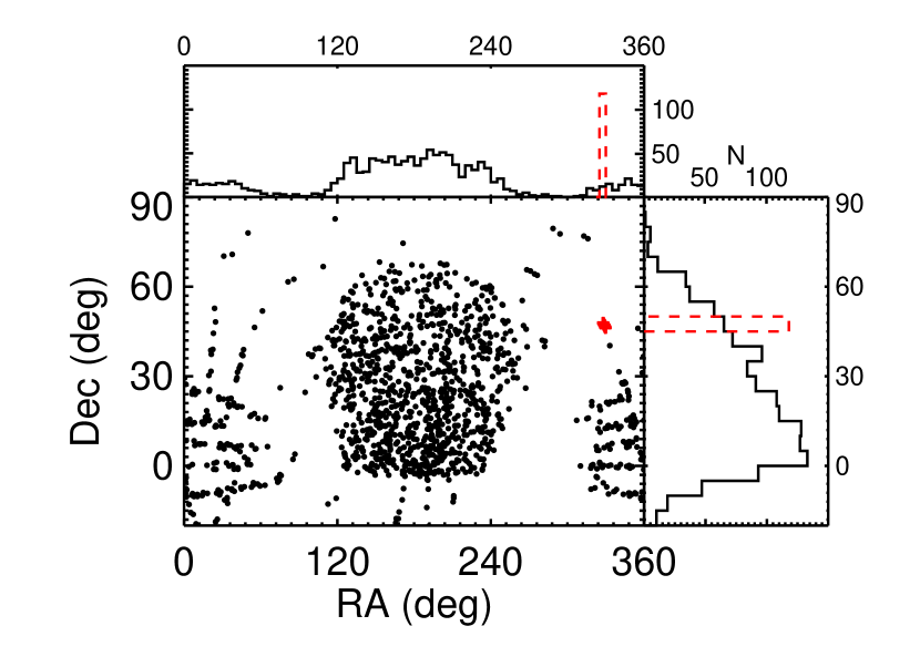
Figure 4.— The spatial distribution of SLoWPoKES binaries, shown in equatorial coordinates, closely follows the SDSS footprint. The upper and right panels show the histogram of Right Ascension and Declination in 5$\arcdeg$ bins. We rejected the 118 CPM candidates found in the direction of open cluster IC 5146 (shown in red pluses and dashed histograms) due to the highly anomalous concentration of pairs and possibly contaminated photometry due to nebulosity (see § 3.1).

Applying these selection criteria to the stellar sample described in § 2.1, we found a total of 3774 wide CPM binary candidates, where each has at least one low-mass component. Among these, we found 118 pairs shown in red pluses and dashed histograms in Figure 4, concentrated in a $20\arcmin\times 150\arcmin$ stripe, in the direction of open cluster IC 5146.As there is significant nebulosity that is not reflected in the extinction values, the photometry and, hence, the calculated photometric distances are not reliable. In addition, while the kinematics are not characteristic of IC 5146, they are more likely to be part of a moving group rather than individual CPM pairs. Thus, we rejected all of these candidates. No other distinct structures, in space and kinematics, were found. Then, we made the quality cuts described in § 2.3 on the companions; 906 and 1085 companions did not meet our threshold for the photometry and proper motions, respectively, and were rejected. The majority of these rejections were near the Galactic Plane, which was expected due to higher stellar density. Thus, at the end, the resulting sample had 1598 CPM double candidates from the statistical matching (Figure 1). Inherent in statistical samples are false positives, arising from chance alignments within the uncertainties of the selection criteria. For any star, the probability of chance alignment grows with the separation making the wider companions much more likely to be chance alignments despite the selection criteria we just implemented. Hence, it is necessary to complete a detailed analysis of the fidelity of the sample.

3.2. Galactic Model: Assessing False Positives in the Binary Sample

To quantitatively assess the fidelity of each binary in our sample, we created a Monte Carlo based Galactic model that mimics the spatial and kinematic stellar distributions of the Milky Way and calculates the likelihood that a given binary could arise by chance from a random alignment of stars. Clearly, for this to work the underlying distribution needs to be carefully constructed such that, as an ensemble, it reflects the statistical properties of the true distribution. The model needs to take into account the changes in the Galactic stellar density and space velocity over the large range of galactocentric distances and heights above/below the Galactic disk plane probed by our sample. Previous studies, focused on nearby binaries, have been able to treat the underlying Galactic stellar distribution as a simple random distribution in two-dimensional space. For example, Lépine & Bongiorno (2007) assigned a random shift of 1–5$\arcdeg$ in Right Ascension for the secondary of their candidate pairs and compared the resultant distribution with the real one. As they noted, the shift cannot be arbitrarily large and needs to be within regions of the sky with similar densities and proper motion systematics. With stars at much larger heliocentric distances in our sample, even a 1$\arcdeg$ shift would correspond to a large shift in Galactic position (1$\arcdeg$ in the sky at 1000 pc represents $\sim$17.5 pc). Therefore, we could not use a similar approach to assess the false positives in our catalog.

The Galactic model is built on the canonical view that the Galaxy comprises three distinct components—the thin disk, the thick disk, and the halo—that can be cleanly segregated by their age, metallicity, and kinematics (Bahcall & Soneira, 1980; Gilmore, Wyse, & Kuijken, 1989; Majewski, 1993). We note that some recent work has argued for the disk to be a continuum instead of two distinct components (Ivezić et al., 2008) or for the halo to be composed of two distinct components (Carollo et al., 2008, 2009). However, for our purposes, the canonical three-component model was sufficient. We also did not try to model the over-densities or under-densities, in positional or kinematic space, caused by co-moving groups, open clusters, star-forming regions, or Galactic streams. If such substructures were found in the SDSS data, they were removed from our sample (see § 3.1). In essence, this model strictly describes stars in the field and produces the three-dimensional position and two-dimensional proper motion, analogous to what is available for the SDSS photometric catalog.

3.2.1 Galactic stellar density profile

In the canonical Galactic model, the stellar densities ($\rho$) of the thin and the thick disks, in standard Galactic coordinates $R$ (Galactic radius) and $Z$ (Galactic height), are given by

$$\rho_{\rm thin}(R,Z) = \rho\ (R_{\odot},0)\ e^{-\frac{|Z|}{H_{\rm thin}}}\ e^{-\frac{|R-R_{\odot}|}{L_{\rm thin}}}$$ (15)

$$\rho_{\rm thick}(R,Z) = \rho\ (R_{\odot},0)\ e^{-\frac{|Z|}{H_{\rm thick}}}\ e^{-\frac{|R-R_{\odot}|}{L_{\rm thick}}},$$ (16)

where $H$ and $L$ represent the scale height above (and below) the plane and the scale length within the plane, respectively. The halo is described by a bi-axial power-law ellipsoid

$$\rho_{\rm halo}(R,Z)=\rho\ (R_{\odot},0)\left(\frac{R_{\odot}}{\sqrt{R^{2}+(Z/q)^{2}}}\right)^{r_{\rm halo}}$$ (17)

with a halo flattening parameter $q$ and a halo density gradient $r_{\rm halo}$. The three profiles are added together, with the appropriate scaling factors, $f$, to give the stellar density profile of the Galaxy:

$$\rho\ (R,Z)=f_{\rm thin}\ \rho_{\rm thin}+f_{\rm thick}\ \rho_{\rm thick}+f_{\rm halo}\ \rho_{\rm halo}.$$ (18)

The scaling factors are normalized such that $f_{\rm thin}+f_{\rm thick}+f_{\rm halo}=1$. With the large number of stars imaged in the SDSS, robust stellar density functions have been measured for the thin and thick disks using the low-mass stars (Jurić et al. 2008; B10) and for the halo using the main-sequence turn-off stars (Jurić et al., 2008). The values measured for the disk in the two studies are in rough agreement. We adopted the disk parameters from B10 and the halo parameters from Jurić et al. (2008); Table 1 summarizes the adopted values.

Table 1Galactic Structure Parameters

Component	Parameter name	Parameter description	Adopted Value
	$\rho\ (R_{\odot},0)$	stellar density	0.0064
	$f_{\rm thin}$	fraction	1-$f_{\rm thick}$-$f_{\rm halo}$
thin disk	$H_{\rm thin}$	scale height	260 pc
	$L_{\rm thin}$	scale length	2500 pc
	$f_{\rm thick}$	fraction	9%
thick disk	$H_{\rm thick}$	scale height	900 pc
	$L_{\rm thick}$	scale length	3500 pc
	$f_{\rm halo}$	fraction	0.25%
halo	$r_{\rm halo}$	density gradient	2.77
	$q\ (=c/a)\tablenotemark{b}$	flattening parameter	0.64

Note. — The parameters were measured using M dwarfs for the disk (Bochanski et al., 2010) and main-sequence turn-off stars for the halo (Jurić et al., 2008) in the SDSS footprint.

3.2.2 Galactic Kinematics

Compared to the positions, the kinematics of the stellar components are not as well characterized; in fact, apart from their large velocity dispersions, little is known about the halo kinematics. We seek to compare the proper motions of a candidate pair with the expected proper motions for that pair given its Galactic position. Thus, we found it prudent to (i) ignore the halo component, with its unconstrained kinematics, at distances where its contributions are expected to be minimal and (ii) limit our model to a distance of 2500 pc, which corresponds to the Galactic height where the number of halo stars begins to outnumber disk stars (Jurić et al., 2008). In practice, all the SLoWPoKES CPM pairs, with the exceptions of subdwarfs for which distances were known to be overestimated, were within $\sim$1200 pc (see Figure 9 below); so we did not introduce any significant systematics with these restrictions.

An ensemble of stars in the Galactic Plane can be characterized as having a purely circular motion with a velocity, $V_{\rm circ}$. The orbits become more elliptic and eccentric over time due to kinematic heating causing the azimuthal velocity, $V_{\phi}$, to decrease with the Galactic height, Z. However, the mean radial ($V_{r}$) and perpendicular ($V_{z}$) velocities for the ensemble at any $Z$ remains zero, with a given dispersion, as there is no net flow of stars in either direction. In addition, this randomization of orbits also causes the asymmetric drift, $V_{\rm a}$, which increases with the age of stellar population and is equivalent to $\sim$10  km s^-1 for M dwarfs. Hence, the velocities of stars in the Galactic disk can be summarized, in Galactic cylindrical coordinates, as:

$$\langle V_{r}~{}(Z)\rangle = 0$$

$$\langle V_{\phi}~{}(Z)\rangle = V_{\rm circ}-V_{\rm a}-f(Z)$$ (19)

$$\langle V_{z}~{}(Z)\rangle = 0,$$

where $V_{\rm circ}=$ 220  km s^-1, $V_{\rm a}=$ 10  km s^-1, $f(Z)=0.013~{}|Z|-1.56\times 10^{-5}~{}|Z|^{2}$ was derived by fitting a polynomial to the data in West et al. (2008), and $Z$ is in parsecs. This formulation of $V_{\phi}(Z)$ is consistent with a stellar population composed of a faster thin disk ($\langle V_{\phi}\rangle=$ 210  km s^-1) and a slower thick disk ($\langle V_{\phi}\rangle=$ 180  km s^-1). Then, we converted these galactocentric polar velocities to the heliocentric, Cartesian UVW velocities. The UVW velocities, when complemented with the dispersions, can be converted to a two-dimensional proper motion (and radial velocity; Johnson & Soderblom, 1987), analogous to our input catalog. We used the UVW velocity dispersions measured for SDSS low-mass dwarfs (Bochanski et al., 2007). All the dispersions were well described by the power-law

$$\sigma(Z)=k\ |Z|^{n},$$ (20)

where the values of constants $k$ and $n$ are summarized in Table 2. As the velocity dispersions in Bochanski et al. (2007) extend only up to $\sim$1200 pc, we extrapolated the above equation for larger distances. While the velocity ellipsoids of F and G dwarfs have been measured to larger distances (e.g. Bond et al., 2009), we preferred to use the values measured for M dwarfs for our low-mass sample.

Table 2Galactic Kinematics

Galactic component	Velocity	k	n
	U	7.09	0.28
thin disk	V	3.20	0.35
	W	3.70	0.31
	U	10.38	0.29
thick disk	V	1.11	0.63
	W	0.31	0.31

Note. — The constants in the power law, $\sigma(Z)=k|Z|^{n}$, that describes the velocity dispersions of the stars in the thin and thick disks. The velocity dispersions were measured from a spectroscopic sample of low-mass dwarfs (Bochanski et al., 2007).

3.2.3 The Model

By definition, a chance alignment occurs because two physically unassociated stars randomly happen to be close together in our line of sight (LOS), within the errors of our measurements. Due to the random nature of these chance alignments, it is not sufficient to estimate the probability of chance alignment along a given LOS simply by integrating Eq. (18). This would tend to underestimate the true number of chance alignments because the density profiles in Eqs. (15–17) are smooth functions that, in themselves, do not include the random scatter about the mean relation that real stars in the real Galaxy have. Thus, the stars need to be randomly redistributed spatially about the average given by Eq. (18) in order to properly account for small, random fluctuations in position and velocity that could give rise to false binaries in our data.

In principle, one could simulate the whole Galaxy in this fashion in order to determine the probabilities of chance alignments as a function of LOS. In practice, this requires exorbitant amounts of computational time and memory. Since our aim was to calculate the likelihood of a false positive along specific LOSs, we, instead, generated stars in much smaller regions of space, corresponding to the specific binaries in our sample. For example, a $30\arcmin\times 30\arcmin$ cone integrated out to a distance of 2500 pc from the Sun will contain at least a few thousand stars within any of the specific LOSs in our sample. The number of stars is large enough to allow for density variations similar to that of the Milky Way while small enough to be simulated with ease. With a sufficient number of Monte Carlo realizations, the random density fluctuations along each LOS can be simulated. We found that $10^{5}$ realizations allowed for the results to converge, within $\sim$0.5%.

We implemented the following recipe to assess the false-positive likelihood for each candidate pair using our Galactic model:

1. The total number of stars in the LOS volume defined by a $30\arcmin\times 30\arcmin$ area, centered on the $\alpha$ and $\delta$ of a given binary, over heliocentric distances of 0–2500 pc was calculated by integrating Eq. (18) in 5 pc deep, discrete cylindrical “cells.”

   Integrating Eq. (18) for $\Delta\theta$ $=$ 30$\arcmin$ and $d=$ 0–2500 pc resulted in $\sim$3300–1580 stars, with the higher numbers more likely to be the LOSs along the Galactic Plane. This number of stars, when randomly redistributed in the entire volume, was more than enough to recreate over-densities and under-densities.

2. The stars were then distributed in three-dimensional space defined by the LOS using the rejection method (Press et al., 1992), generating $\alpha$, $\delta$, and $d$ for each star. The rejection method ensured that the stars were randomly distributed while following the overlying distribution function, which, in this case, was the stellar density profile given by Eq. (18).

   The model did an excellent job of replicating the actual distribution of stars in the three-dimensional space. The red histograms in Figure 5 show the number of stars from the center of the LOS as a function of angular separation for the model (dashed lines) and the data (solid lines), averaged over all LOSs where candidate binaries were identified in § 3.1. There is an excess of pairs at close separations, a signature of genuine, physically associated pairs, while the two distributions follow the same functional form at larger separations, where chance alignments dominate. The increasing number of pairs with angular separation is an evidence of larger volume that is being searched. Integrating the model predicts $\sim$8.0 stars within a search radius of 60$\arcsec$ and $\sim$71 within 180$\arcsec$. In other words, for a typical LOS with candidate binaries, we would, on average, expect to find 8 chance alignments within 60$\arcsec$ and $\sim$71 within 180$\arcsec$ when considering only angular separation.

   For the 180$\arcsec$ radius around each LOS, the average number of stars in the model and the data were within a few $\sigma$ of each other, with the largest deviations found along the LOSs at low Galactic latitudes or large distances. As our model only integrated to $d=$ 2500 pc, deviations for LOSs at large distances were expected. Deviations for LOSs at low Galactic latitudes are reasonable as the parameters in Eqs. (15) and (16) as not as well constrained along the Galactic disk. Hence, we concluded that the rejection method used in redistributing the stars in the $30\arcmin\times 30\arcmin$ LOS is correctly implemented and that the model successfully replicates the three dimensional spatial distribution of the stars in the Galaxy.

   When the distances were matched, the number of pairs decreased as chance alignments were rejected (blue histograms in Figure 5); there are, on average, only $\sim$0.41 and $\sim$3.6 chance alignments within 60$\arcsec$ and 180$\arcsec$, respectively. Note that matching distances, in addition to the angular separation, significantly enhanced the peak at the small separations.

   

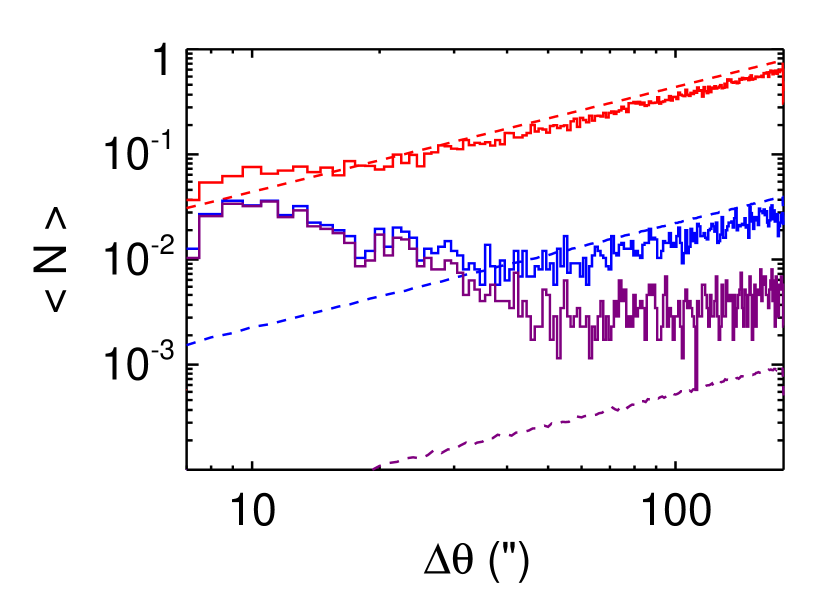
   Figure 5.— The distribution of the (average) number of stars found around the LOSs around our binary candidates as calculated from the SDSS DR7 data (solid histograms) and our Galactic model (dashed histograms). All optical pairs (red), pairs with matching distances (blue), and pairs with matching distances and proper motion components (purple) are shown. The excess at small separations, a signature of real pairs, is enhanced as additional properties are matched. Unlike the rest of the paper, we counted all stars with $r\leq$ 22.5, without any quality cuts, for this plot to do a realistic comparison with the model. Note that $\langle N\rangle$ denotes the number of stars found at that angular separation (counted in 1$\arcsec$ bins). We used the raw parameters for the Galactic model (Jurić et al. 2008, B10). As a whole, the model does an excellent job of mimicking the number of stars and their spatial and kinematic distribution in the Milky Way along typical SDSS LOSs.

3. Based on the Galactic position of each randomly generated star, mean UVW space velocities and their dispersions were generated based on Eq. (3.2.2) and Eq. (20), respectively. Proper motions were then calculated by using the inverse of the algorithm outlined in Johnson & Soderblom (1987). These generated proper motions represent the expected kinematics of stars at the given Galactic position.

   Figure 6 shows the comparison between the proper motions in the SDSS/USNO-B catalog and our model; component proper motions of stars within 60$\arcmin$ of all LOSs, where candidate pairs were found. For the purposes of this plot, we restricted the stars to be within 1200 pc and of spectral type K5 or later so we could compare kinematics with a sample similar to our resultant catalog. We also did not compare the distributions at $\mu_{\alpha}$ or $\mu_{\delta}$ $<$ 10 mas yr^-1where the proper motions are comparable to the 1-$\sigma$ errors and, hence, not reliable. Since our initial sample was has $\mu\geq$ 40 mas yr^-1, stars with the small proper motion component are either rejected or their motion is dominated by the other component in our analysis. As evidenced in the figure, our model reproduced the overall kinematic structure of the thin and thick disks.

   

   Figure 6.— Proper motion distributions for stars within 60$\arcmin$ of LOSs along all identified candidate pairs in SDSS/USNO-B (solid histograms) and in our Galactic model (dashed histograms). For the purposes of this plot, we restricted the stars to be of spectral types K5 or later and be within 1200 pc to avoid being skewed by systematic differences. In addition, we do not compare proper motion components $<$ 10 mas yr^-1 as they comparable to the 1-$\sigma$ errors and, hence, not reliable (see text). Again, the kinematics of the thin and thick disk of the Milky Way are very well reproduced by our Monte Carlo model.

   When the proper motions were matched (purple histograms in Figure 5), in addition to the angular separation and distances, the number of chance alignments fell drastically, especially at the smaller separations. In fact, at $\Delta\theta$ $\leq$ 15$\arcsec$, there were $<10^{-4}$ chance alignments, on average; even at $\Delta\theta$$=$ 180$\arcsec$, the real pairs outnumbered the chance alignments by a factor of 4–5. Cumulatively, for a typical LOS, there were, on average, only $\sim$0.0097 and $\sim$0.086 chance alignments within 60$\arcsec$ and 180$\arcsec$, respectively. As a result of matching distance and proper motions components, the number of chance alignments within 180$\arcsec$ were reduced by a factor of $\sim$800.

4. In the model galaxy, we repeated the selection process used to find CPM pairs in the SDSS photometric catalog, as described in § 3.1. To avoid double-counting, the input coordinates of the LOS were considered to be the primary star. Note that we did not intend to model and reproduce both stars of a given pair but wanted to see if a random chance alignment could produce a companion for a given primary. Hence, each additional star that was found to satisfy Eqs. (13) and (14) was counted as an optical companion. The average number of companions found in the $10^{5}$ Monte Carlo realizations is the probability of chance alignment or the probability that the candidate pair is a false positive, P_f, for that candidate pair. The number of realizations sets the resolution of P_f at 10^-5.

5. Finally, this was repeated for all candidate pairs that were found in § 3.1. Figure 7 shows the distribution of P_f all of the candidate pairs; we further discuss this distribution is § 3.3.

To conclude, the result of our Galactic model was a $30\arcmin\times 30\arcmin$ area of the sky, centered around the given CPM pair, with the surrounding stars following the Galactic spatial and kinematic distributions of the Milky Way. Each star in this model galaxy was described by its position ($\alpha$, $\delta$, and $d$) and proper motion ($\mu_{\alpha}$and $\mu_{\delta}$), same as is available for SDSS photometric catalog. Based on the above results, we concluded that the Galactic model sufficiently reproduced the five-dimensional (three spatial and two kinematic) distribution of stars along typical LOSs in the Milky Way and, thus, allowed for the calculation of probability that a given CPM double is a chance alignment.

3.3. Fidelity

As described in the previous section, we have implemented a very stringent selection algorithm in identifying the CPM pairs. In addition to only including objects with the most robust photometry and proper motions, we also used a relatively high proper motion cut of $\mu\geq$ 40 mas yr^-1 for the input sample, which considerably decreased the number of low-mass stars. As described above, an algorithm optimized to reject the most false positives, even at the expense of real pairs, was used in the statistical matching of angular separation, photometric distance, and proper motion components. Lastly, we used the Galactic model to quantify the probability of chance alignment, P_f, for each of the 1558 candidate pairs.

Normally all candidate pairs with P_f $\leq$ 0.5, i.e. a higher chance of being a real rather than a fake pair, could be used to identify the binaries. However, to minimize the number of spurious pairs, we required

$$P_{\rm f}\leq 0.05.\\$$ (21)

for a pair to be classified as real. Here we note that P_f represents the false-alarm probability that a candidate pair identified by matching angular separation, photometric distance, and proper motion components, as described by Eqs. (13) and (14), is a real pair; it is not the probability that a random low-mass star is part of a wide binary.

Making the above cut on P_f  resulted in a catalog of 1342 pairs, with a maximum of 5% or 67 of the pairs expected to be false positives. However, as a large number of the pairs have extremely small P_f (see Figure 7), the number of false positives is likely to be much smaller. Adding up the P_f for the pairs included in the catalog gives an estimated 22 (1.65%) false positives. In other words, the overall fidelity of SLoWPoKES is 98.35%. This is a remarkably small proportion for a sample of very wide pairs, especially since they span a large range in heliocentric distances and is a testament to our selection criteria. For example, if the proper motion components were matched to within 2 $\sigma$, Eq. (21) would have rejected $\gtrsim$ 60% of the candidates. Our choice of Eq. (21) is a matter of preference; if a more efficient (or larger) sample is needed, it can be changed to suit the purpose.

Figure 7.— The probability of chance alignment (P_f) for candidate SLoWPoKES pairs based on their positions and kinematics, as calculated by our Galactic model. We adopted P_f $=$ 0.05 (dotted line) as our threshold for inclusion in the SLoWPoKES catalog. The resolution of the Monte Carlo simulation is $10^{-5}$, which causes the peak at $\log$ P_f $=10^{-5}$.

To get a first-order approximation of how many real binaries we are missing or rejecting, we applied our selection algorithm to the rNLTT CPM catalog with 1147 pairs (Chanamé & Gould, 2004). Note that Chanamé & Gould (2004) did not match distances of the components, as they did not have reliable distance estimates available and matched total proper motions instead of a two-dimensional vector matching in our approach. Out of the 307 rNLTT pairs, which have $\Delta\theta\leq 180\arcsec$ and are within the SDSS footprint, we recover both components of 194 systems (63%) and one component of another 56 (18%) systems, within 2$\arcsec$ of the rNLTT coordinates. Of the 194 pairs for which both components had SDSS counterparts, 59 (30%) pairs satisfied our criteria for proper motions, Eq. (14), while 19 (10%) pairs satisfied our criteria for both proper motions and distances, Eqs. (13) and (14). In other words with our selection criteria, we recovered only 10% of the rNLTT pairs, with SDSS counterparts, as real binaries. If we relax our selection criteria to match within 2-$\sigma$, the number of recovered pairs increases to 82 with matching proper motions and 37 with matching proper motions and distances. Of course, as the rNLTT is a nearby, high proper motion catalog, Chanamé & Gould (2004) had to allow for larger differences in proper motions due to the stars’ orbital motion, which is not applicable to the SLoWPoKES sample (see § 3.1). In conclusion, compared to previous catalogs of CPM doubles, we find a small fraction of previously identified very wide binaries. The reasons for the low recovery rate are two-fold: (i) the restrictive nature of our matching algorithm that rejects the most false positives, even at the expense of real pairs and (ii) improvement in the identification method—e.g. matching proper motions in vector space and being able to use photometric distance as an additional criterion.

Table 3Properties of SLoWPoKES pairs

ID	Position (J2000)					Photometry
	$\alpha_{A}$	$\delta_{A}$	$\alpha_{B}$	$\delta_{B}$		$r_{A}$	$i_{A}$	$z_{A}$	$r_{B}$	$i_{B}$	$z_{B}$
SLW	(deg)					(mag)
J0002+29	0.515839	29.475183	0.514769	29.470617		16.79 (0.02)	15.85 (0.02)	15.33 (0.02)	19.35 (0.02)	17.91 (0.02)	17.17 (0.02)
J0004-10	1.122441	-10.324043	1.095927	-10.296753		18.25 (0.02)	17.08 (0.02)	16.46 (0.02)	18.66 (0.02)	17.42 (0.02)	16.70 (0.02)
J0004-05	1.223125	-5.266612	1.249632	-5.237299		14.85 (0.01)	14.31 (0.01)	14.02 (0.02)	19.56 (0.02)	18.10 (0.01)	17.31 (0.02)
J0005-07	1.442631	-7.569930	1.398478	-7.569359		17.35 (0.02)	16.25 (0.01)	15.65 (0.01)	18.78 (0.02)	17.43 (0.02)	16.69 (0.01)
J0005+27	1.464802	27.325805	1.422484	27.300282		18.91 (0.02)	17.63 (0.02)	16.94 (0.01)	19.79 (0.02)	18.29 (0.02)	17.50 (0.02)
J0006-03	1.640868	-3.928988	1.641011	-3.926589		17.06 (0.01)	16.01 (0.02)	15.44 (0.01)	17.88 (0.01)	16.62 (0.02)	15.93 (0.01)
J0006+08	1.670973	8.454040	1.690136	8.498541		19.48 (0.02)	18.14 (0.02)	17.45 (0.02)	19.57 (0.02)	18.15 (0.01)	17.43 (0.02)
J0007-10	1.917002	-10.340915	1.924510	-10.338869		17.43 (0.01)	16.50 (0.01)	16.02 (0.03)	18.33 (0.01)	17.24 (0.01)	16.66 (0.03)
J0008-07	2.135590	-7.992694	2.133660	-7.995245		17.33 (0.01)	16.35 (0.02)	15.86 (0.02)	18.14 (0.01)	16.98 (0.02)	16.36 (0.02)
J0009+15	2.268841	15.069630	2.272453	15.066457		18.52 (0.02)	17.00 (0.02)	16.09 (0.01)	18.39 (0.02)	16.83 (0.02)	15.95 (0.01)

Table 3

Proper Motion					Distance			Spectral Type			Binary Information
$\mu_{\alpha_{A}}$	$\mu_{\delta_{A}}$	$\mu_{\alpha_{B}}$	$\mu_{\delta_{B}}$		$d_{A}$	$d_{B}$		$A$	$B$		$\Delta\theta$	$\Delta\mu$	$\Delta d$	BE	Pf	Class
( mas yr-1)					(pc)						($\arcsec$)	( mas yr-1)	(pc)	($10^{40}$ ergs)	(%)
198 (2)	38 (2)	197 (3)	35 (3)		341	301		M1.7	M3.6		16.8	2.9	39	58.08	0.000	SD
43 (3)	-4 (3)	36 (4)	-8 (4)		362	338		M2.7	M3.1		135.9	7.5	23	3.94	0.036	DD
101 (2)	11 (2)	99 (4)	8 (4)		301	333		K7.1	M3.8		142.0	3.1	31	13.45	0.006	DD
30 (2)	-21 (2)	30 (3)	-27 (3)		296	273		M2.4	M3.4		157.6	6.0	23	4.90	0.015	DD
10 (3)	-40 (3)	5 (4)	-40 (4)		357	380		M3.1	M3.9		163.6	5.5	22	2.26	0.037	DD
-40 (2)	-35 (2)	-40 (2)	-31 (2)		242	270		M2.2	M3.1		8.7	3.9	27	112.47	0.005	DD
-48 (4)	-5 (4)	-41 (4)	-3 (4)		417	476		M3.3	M3.5		174.1	7.5	58	1.59	0.033	DD
37 (3)	34 (3)	42 (4)	31 (4)		429	445		M1.5	M2.3		27.6	5.6	16	27.74	0.034	DD
-9 (2)	-42 (2)	-7 (3)	-41 (3)		344	379		M1.7	M2.7		11.5	2.3	34	74.69	0.017	DD
36 (3)	-16 (3)	37 (3)	-21 (3)		150	161		M4.2	M4.2		17.0	4.8	11	21.02	0.004	DD

Note. — The first 10 pairs are listed here; the full version of the table is available online.

4. Characteristics of the SLoWPoKES catalog

Using statistical matching of angular separation, photometric distance, and proper motion components, we have identified 1598 very wide, CPM double candidates from SDSS DR7. We have built a Galactic model, based on empirical measurements of the stellar density profile and kinematics, to quantitatively evaluate the probability that each of those candidate doubles are real (Figure 7). Using Eq. (21), we classify 1342 pairs as real, associated pairs. In deference to their extremely slow movement around each other, we dub the resulting catalog SLoWPoKES for Sloan Low-mass Wide Pairs of Kinematically Equivalent Stars. Table 3 lists the properties of the identified pairs. The full catalog is publicly available on the world wide web. SLoWPoKES is intended to be a “live” catalog of wide, low-mass pairs, i.e., it will be updated as more pairs are identified and as follow-up photometric and spectroscopic data become available.

Figure 8 shows a collage of $gri$ composite images, 50$\arcsec$ on a side, of a selection of representative SLoWPoKES systems; the images are from the SDSS database. In the collage high-mass ratio pairs (top row; mass ratio = $m_{2}/m_{1}<0.5$), equal-mass pairs (middle row; having masses within $\sim$5% of each other), white dwarf–disk dwarf pairs (bottom row, left), and halo subdwarf pairs (bottom row, right) are shown. Table 5 summarizes the different types of systems in the catalog.

Table 5The SLoWPoKES binaries

Class	Type	Number
DD	disk dwarf	1245
SD	subdwarf	70
WD	white dwarf–disk dwarf	21
T	triple	4

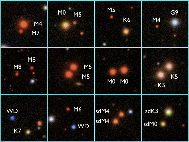
Figure 8.— $50\arcsec\times 50\arcsec gri$ composite images of CPM pairs found in the SLoWPoKES survey. Pictured are high-mass ratio pairs (top row), identical twins (middle row), white dwarf–disk dwarf pairs (bottom row, left), and halo subdwarf pairs (bottom row, right). Spectral types, based on their $r-z$ colors are shown. Overall, 1342 wide, low-mass binaries were identified.

In the sections that follow, we summarize various aspects of the systems that constitute the SLoWPoKES catalog and briefly examine some of the follow-up science that can be pursued with SLoWPoKES. We wish to emphasize that the SLoWPoKES catalog is intended principally as a high-fidelity sample of CPM doubles that can be used for a variety of follow-up investigations where the reliability of each object in the catalog is more important than sample completeness. Thus, we have not attempted to fully account for all sources of incompleteness or bias; and we intentionally have not applied any form of statistical “corrections” to the catalog.

We note that some of the most important sources of incompleteness in the present catalog could be at least partially overcome with follow-up observations. For example, the principal incompleteness in SLoWPoKES arises from the lack of proper motions for SDSS stars that were not detected in USNO-B. Proper motions either do not exist or are not reliable for stars (i) fainter than $r=$ 20 or (ii) within 7$\arcsec$ of a brighter star. The first criterion currently rules out most of the mid–late M dwarf companions, while the latter rejects close binaries and most hierarchical higher-order systems. However, as the SDSS photometric and astrometric data are available for these systems, their multiplicity could be verified with more rigorous analysis or through cross-matching with other catalogs. For example, by cross-matching SDSS with 2MASS, an M4.5–L5 binary (Radigan et al., 2008) and an M6–M7 binary (Radigan et al., 2009) have already been identified. At the other end of the spectrum, SDSS saturates at $r\approx$ 14, resulting in saturated or unreliable photometry for the brighter stars. We found that more than 1000 candidate pairs were rejected for this reason; with reliable follow-up photometry these could be added as additional genuine SLoWPoKES binaries.

Even so, a fully volume-complete sample is likely to be impossible to compile over the full ranges of spectral types and distances spanned by our catalog. For example, our magnitude limits of 14 $\lesssim r\leq$ 20 imply that while we are sensitive to K5 dwarfs at $\sim$250–3900 pc, we are sensitive to M5 dwarfs at $\sim$14–180 pc. This means (i) we are entirely insensitive to pairs with the most extreme mass ratios (i.e. a K5 paired with an M6 or M7) and (ii) we cannot directly compare the properties of K5 and M5 spectral subtypes in identical distance ranges. In addition, as illustrated in Figure 9, with our 7$\arcsec\leq\Delta\theta\leq$ 180$\arcsec$ search radius we are sensitive to companions with separations of $\sim$700–18000 AU at 100 pc but $\sim$7000–180000 AU at 1000 pc. Thus, it is important with the current catalog that statistical determinations of ensemble system properties be performed within narrowly defined slices of separation and distance. We do so in the following subsections as appropriate; but we emphasize again that our intent here is primarily to characterize the SLoWPoKES sample and will proffer any interpretive conclusions only tentatively.

Finally, as is evident from Table 5, the current SLoWPoKES catalog is clearly not well suited for study of higher-order multiples (i.e. triples, quadruples, etc.). Identifying CPM higher-order multiple systems in SDSS is very challenging due to the lack of reliable proper motions in the SDSS/USNO-B matched catalog at $\Delta\theta<7\arcsec$ and $r>$ 20. Unless all components are widely separated and are all bright, they will be rejected in our search. In addition, we are currently rejecting hierarchical triples consisting of a close pair that is unresolved in SDSS and a wide, CPM tertiary. If the mass ratio of the close, unresolved pair is near unity, it will appear as an over-luminous single star that will then be misinterpreted by our algorithm as having a discrepant photometric distance from its wide tertiary companion. The available SDSS photometry and astrometry shows evidence of a substantial number of such multiple systems, and we plan to make these the subject of a future study. Already, four CPM triples are identified in our search (Table 5). Moreover, the current SLoWPoKES catalog is likely to contain quadruple systems in which the two components of the identified wide binary are themselves in fact spatially unresolved binaries with near-equal mass components. We have initiated an adaptive optics program to identify such higher-order systems in the SLoWPoKES catalog.

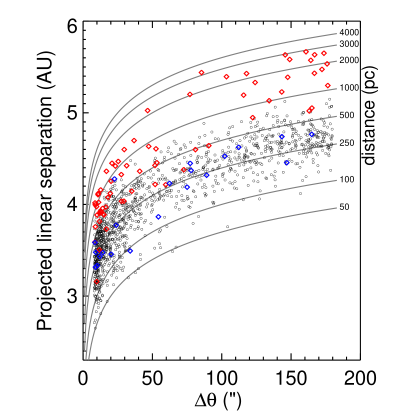
Figure 9.— The projected linear separation of SLoWPoKES pairs are plotted as a function of angular separation, with the iso-distance lines plotted across the grid. DD (black), SD (red), and WD–DD pairs (blue) are shown. Systematically larger distances for the SDs is clearly seen, which is expected as photometric DD photometric parallax relations were used to calculate the SD distances as well. Hence, SDs are excluded in all analysis involving their distances.

4.1. Kinematic Populations

Luyten (1922) devised the reduced proper motion (RPM) diagram to be used in the stead of the H-R diagram when distances to the objects are not available, as is the case in large imaging surveys. The RPM of an object is defined as

$${\rm H}\equiv m+5~{}\log\mu+5=M+5~{}\log v_{\rm t}-3.25$$ (22)

where $v_{\rm t}$ is the heliocentric tangential velocity in  km s^-1 given by $v_{\rm t}=4.74~{}\mu~{}d$ and $\mu$ is the proper motion in arcseconds yr^-1. Just as in a H-R diagram, the RPM diagram effectively segregates the various luminosity or kinematic classes from each other (e.g. Chanamé & Gould 2004; Harris et al. 2006; Lépine & Bongiorno 2007; SIJ08).

WDs, in addition to being relatively very blue, are less luminous than either the DDs or the SDs; hence, the observed WDs tend to be nearby disk WDs with high tangential velocities. Specifically, spectroscopic follow-up has shown that the disk WDs with $v_{\rm t}=$ 25–150  km s^-1 (Figure 10, black dashed lines) can be effectively identified from the $g$-band RPM diagram, when complemented by photometric parallax relations (Kilic et al., 2006). However, we note that spectroscopic follow-up is needed to confirm that the identified objects are actually WDs. The available SDSS spectra confirm that 9 of the 21 WD primaries, identified in SLoWPoKES, are indeed WDs. As the WDs were identified from the $g$-band, they scatter toward the SD and DD locus in the $r$-band RPM diagram.

Subdwarfs are low-metallicity halo counterparts of the MS dwarfs found in the Galactic disk. Hence, they have bluer colors at a given absolute magnitude (however, the $g-r$ colors for M subdwarfs are redder; West et al., 2004; Lépine & Scholz, 2008) and have higher velocity dispersions. As a result, the subdwarfs lie below the disk dwarfs in the RPM diagram. To segregate the SDs from the DDs, we used the DD photometric parallax relations complemented by the mean tangential velocity of halo stars, $v_{\rm t}=$ 180  km s^-1. This relation is shown in blue dashed lines in the $r$-band RPM diagram in Figure 10. As the mean halo velocity was used, SDs can scatter above the line; but DDs would not be expected to be below the blue line. For comparison, $v_{\rm t}=$ 25  km s^-1, the mean tangential velocity of disk stars, is also shown. Note that DDs in SLoWPoKES have tangential velocities larger than the mean velocity of the disk, which is expected as we rejected all stars with $\mu<$ 40  mas yr^-1.

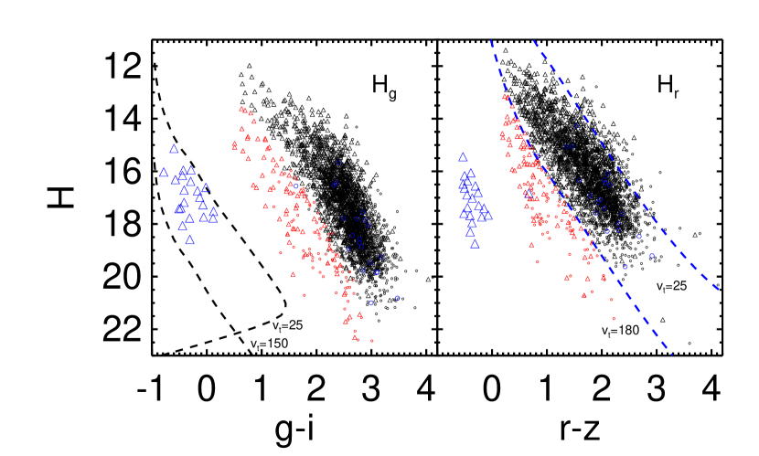
Figure 10.— SLoWPoKES pairs plotted in the H_g vs. $g-i$ (left) and H_r vs. $r-z$ RPM diagrams; primaries (triangles) and secondaries (circles) of DD (black), SD (red), and WD–DD (blue) pairs are shown. The WDs are identified from the $g$-band RPM diagram, complemented by $M_{g}(g-i)$ for WDs, as having 25 $<v_{\rm t}<$ 150  km s^-1 (black dashed lines) and are all expected to be part of the disk population. SDs are segregated from the DDs using the $r$-band RPM diagram, assuming SDs have $v_{\rm t}>$ 180  km s^-1 (blue dashed line) and the DD photometric parallax relations.

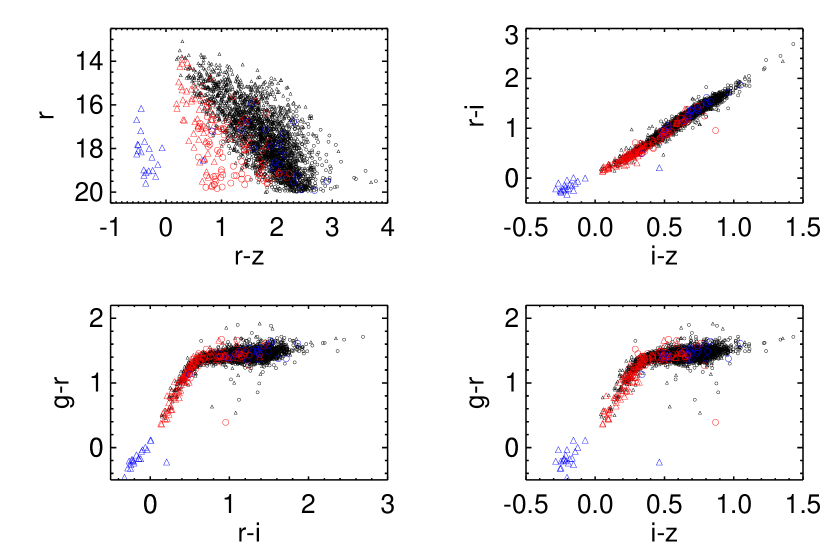
Figure 11.— $r$ vs. $r-z$ Hess diagram and color-color plots for the SLoWPoKES catalog; shown are the primary (triangles) and secondaries (circles) for DD (black), SD (red), and WD–DD pairs (blue). The subdwarfs are mostly of K spectral type and do not show redder $g-r$ colors at given $r-i$ or $i-z$ colors, as seen in M subdwarfs (West et al., 2004; Lépine & Scholz, 2008).

Figure 10 shows the H_g vs. $g-i$ and H_r vs. $r-z$ RPM diagrams with both the primary (triangle) and the secondary component (circle) for the 21 WD–DD (blue), 70 SD–SD (red), and 1245 DD–DD (black) pairs that were identified in SLoWPoKES. The properties of the DDs, SDs, and WDs in various color-magnitude and color-color planes are compared in Figure 11. The identified SDs are either K or early-M spectral types, as our magnitude and color limits exclude the M subdwarf locus. The overestimation in the distances to SDs is clearly evident in Figure 9, as they are at systematically larger distances relative to the DDs. As a result, the calculated physical separations for the SDs are also systematically larger. At present a substantial number of subdwarf candidates are rejected from SLoWPoKES because the overestimated distances result in $\Delta d>$ 100 pc.

RPM diagrams have been used to confirm the binarity of CPM pairs in the past (e.g. Chanamé & Gould, 2004). As components of a binary system most probably formed from the same material and at the same time, they should be members of the same luminosity class (with the obvious exception of WD–DD pairs) and the line joining the components should be parallel to the track in which the systems reside. In the case of WD–DD dwarf systems or systems that have separations comparable to the error bars in the RPM diagram, the line need not be parallel. The $r$-band RPM diagram, in Figure 12, confirms that the SLoWPoKES systems are associated pairs.

Figure 12.— A randomly selected sample of SLoWPoKES pairs plotted on the RPM diagram; components of DD (dotted), SD (solid), and WD–DD (dashed) pairs are connected. As binaries are expected to be part of the same kinematic populations, they are expected to lie parallel to the dwarf/subdwarf tracks with the obvious exception of WD–DD pairs or when the two components lie within the error bars of each other.

4.2. Separation

Despite the large number of optical companions found at larger angular separations, the final distribution of the identified pairs is mostly of pairs with small angular separations. This is shown in Figure 13 where, after a narrow peak at $\Delta\theta\sim 15\arcsec$, the distribution tapers off and rises gently after $\Delta\theta\gtrsim 70\arcsec$. To convert the angular separations into physical separations, we need to account for the projection effects of the binary orbit. As that information for each CPM pair is not available, we apply the statistical correction between projected separation ($s$) and true separation ($a$) determined by FM92 from Monte Carlo simulations over a full suite of binary parameters. They found that

$$a\approx 1.26\ s=1.26\ \Delta\theta\ d$$ (23)

where the calculated $a$ is the physical separation including corrections for both inclination angle and eccentricity of the binary orbit and is the actual semi-major axis. We emphasize, however, that these $a$ values are valid only for ensemble comparisons and should not be taken as an accurate measure of $a$ for any individual system. In addition, the above equation implies that, at the extrema of angular separations probed, we are biased towards systems that are favorably oriented, either because of $\sin i$ projection effects or eccentricity effects that lead to a changing physical separation as a function of orbital position. For example, at $\Delta\theta$ $\approxeq 7\arcsec$, pairs at their maximal apparent separation are more likely to be identified while we are biased towards pairs with smaller apparent separations at $\Delta\theta$ $\approxeq 180\arcsec$.

Figure 13.— The projected angular separation (left) and the semi-major axes (right; corrected using $a=1.26\ \theta\ d$, FM92, ) for the CPM doubles identified in SLoWPoKES. The upper x-axis in the right panel shows the semi-major axis in parsecs; the widest CPM pairs known in the literature (see Table 4.2) are shown as pluses at their semi-major axis values at the top of the panel. SDs were excluded from the right panel. The distribution of physical separations is clearly bimodal with a break at $\sim$0.1 pc.

The distribution of $a$ is plotted for the SLoWPoKES sample in Figure 13 (right). The semi-major axes for the identified pairs range from $\sim 10^{3}-10^{5}$ AU ($\sim$0.005–0.5 pc), with sharp cutoffs at both ends of the distribution, and with a clear bimodal structure in between. The cutoff at small separations is observational, resulting from our bias against angular separations $\Delta\theta<7\arcsec$. Indeed, the range of physical separations probed by SLoWPoKES is at the tail-end of the log-normal distribution ($\langle a\rangle=$ 30 AU, $\sigma_{\log a}=$ 1.5) proposed by DM91 and FM92. The cutoff we observe at the other end of the distribution, $a\sim 10^{5}$ AU, is likely physical. With the mean radii of prestellar cores observed to be around 0.35 pc or $10^{4.9}$ AU (Benson & Myers, 1989; Clemens et al., 1991; Jessop & Ward-Thompson, 2000), SLoWPoKES represents some of the widest binaries that can be formed. However, other studies have found binary systems at similar separations; plotted in pluses are the wide CPM pairs compiled from the literature and listed in Table 4.2.

Table 6A sub-sample of previously known wide binaries with the projected separation, $s$, $\gtrsim 10^{4}$ AU ($\sim$0.05 pc)

ID		$\Delta\theta$	$s$	Spectral Type		BE	References
Primary	Secondary	(″)	(AU)	Primary	Secondary	($10^{40}$ ergs)
HIP 38602	LSPM J0753+5845	109.90	10175	G8.1	M5.1	132.18	1
HIP 25278	HIP 25220	707.10	10249	F1.8	K5.8	307.44	1
HIP 52469	HIP 52498	288.00	10285	A8.9	F9.3	379.74	1
HIP 86036	HIP 86087	737.90	10400	F8.4	M2.6	184.33	1
HIP 58939	LSPM J1205+1931	117.20	10558	K0.5	M4.7	107.44	1
HIP 51669	LSPM J1033+4722	164.30	10668	K7.3	M5.7	52.10	1
HIP 81023	LSPM J1633+0311N	252.00	10723	K3.2	M3.8	81.51	1
HIP 50802	LSPM J1022+1204	311.90	11139	K5.9	M3.1	56.44	1
HIP 78128	LSPM J1557+0745	144.60	11385	G7.1	M5.0	123.01	1
HIP 116106	2MASS J2331-04AB	451.00	11900	F8	$\cdots$	161.10	2
$\alpha$ Cen AB	NLTT 37460	9302.00	12000	G2+K1	M6	430.21	3

References. — (1) Lépine & Bongiorno (2007); (2) Caballero (2007); (3) Caballero (2009); (4) Caballero (2010); (5) Bahcall & Soneira (1981); (6) Latham et al. (1984); (7) Makarov et al. (2008); (8) Zapatero Osorio & Martín (2004); (9) Faherty et al. (2010); (10) Chanamé & Gould (2004); (11) Quinn et al. (2009); (12) Poveda et al. (2009); (13) Allen et al. (2000).

Note. — The first 10 pairs are listed here; the full version of the table is available online.

Between the cutoffs at $\sim 10^{3}$ AU and at $\sim 10^{5}$ AU, we observe a distinct bimodality in the distribution of physical separations at $a\sim 10^{4.2}$ AU ($\sim$0.1 pc) that has no correlation with the distance to the observed system (see § 5 below). We have high confidence that this bimodality is not due to some sort of bias in our sample. As discussed above, the most important observational bias affecting the distribution is the bias against pairs with $a\lesssim 10^{3}$ AU, because we are not sensitive to systems with $\Delta\theta<7\arcsec$ nor to very nearby systems. In addition, given the care with which we have eliminated false positives in the sample, we have high confidence that the bimodal structure is not due to a large contamination of very wide chance pairs. Instead, it is likely that this bimodality reveals two distinct populations of wide binaries in SLoWPoKES, possibly representing systems that form and/or dissipate through differing mechanisms. We discuss the bimodality in the context of models of binary formation and kinematic evolution in § 5.

4.3. Mass Distribution

Figure 14 (left panel) shows the $r-z$ color distributions of the primary and secondary components of SLoWPoKES pairs, where the primary is defined as the component with the bluer $r-z$ color (and, thus, presumably more massive). As the SLoWPoKES sample is dominated by dwarfs, the $r-z$ color distribution should correspond directly to the mass distribution. Both the primary and secondary distributions show a peak at the early–mid M spectral types (as inferred from their colors; § 2.4.2), probably due to, at least in part, the input sample being mostly M0–M4 dwarfs. However, apart from the saturation at $r\lesssim$ 14, there is no bias against finding higher-mass companions. Hence, it is notable that more than half of the primaries have inferred spectral types of M0 or later, with the distribution of the secondaries even more strongly skewed to later spectral types (by definition).

Figure 14.— Left: The $r-z$ color for the primaries (solid) and secondaries (dashed). The upper x-axis, in the left panel, shows the spectral types inferred from their $r-z$ colors (Covey et al., 2007; West et al., 2008). Both distributions exhibit bimodality and are, similar to each other. Right: The mass ratio, $q\equiv M_{2}/M_{1}$ for SLoWPoKES pairs (solid histogram) indicates that most are in equal- or near-equal-mass systems. Within the observational limits of SDSS, we should have been able to see much more extreme mass ratio systems (dashed histogram). The lack of such systems indicates that the observed distribution is not dominated by observational biases and is probably real.

As discussed above, selection biases in SLoWPoKES are in general a function of distance because of the large range of distances probed (see Sec. 4.1; Figures 3 and 9). Thus, in Figure 15 we show the box-and-whisker plot of the distribution of the $r-z$ colors of the primary (blue) and secondary (red) components as a function of distance in 100 pc bins. The bar inside the box is the median of the distribution; the boxes show the inter-quartile range (defined as the range between 25^th and 75^th percentiles); the whiskers extend to either the 1.5 times the inter-quartile range or the maximum or the minimum value of the data, whichever is larger; and the open circles show the outliers of the distribution. The black dashed lines show the bright and faint limits of our sample ($14\lesssim r\leq 20$). As the figure indicates the primary and secondary distributions are bluer at increasing distances, as would be expected due to the bright and faint limits; but the secondary distribution does not change as compared to the primary distribution as a function of distance. However, this is likely to be a strict function of the faintness limit of our catalog: the stellar mass function peaks around M4 spectral type (B10) while we cannot see M4 or later stars beyond $\sim$400 pc. Hence, with our current sample, we cannot discern whether the tendency for the secondary distribution to follow the primary distribution is a tendency toward $q\sim 1$ or a tendency for the secondary distribution to be drawn from the field mass function.

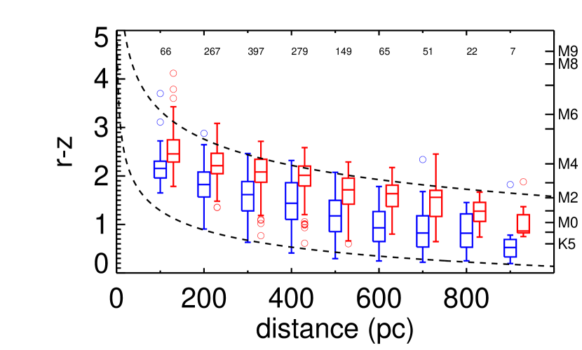
Figure 15.— The color distribution for the primary (blue) and secondary (red) components of SLoWPoKES pairs as a function of distance, in 100 pc bins shown in a box-and-whisker plot; the number of pairs in each bin is printed along the top. The bar inside the boxes show the median of the distribution; the boxes show the inter-quartile range; the whiskers extend to either 1.5 times the inter-quartile range or the maximum or the minimum value of the data, whichever is larger; and the open circles show the outliers. The dashed lines show the magnitude limits of this catalog ($14\lesssim r\leq 20$). The secondary distribution tracks the primary distribution at all distances.

We can also examine the distribution of the secondary masses relative to their primaries, i.e. the mass ratio distribution, which is an important parameter in the study of binary star formation and evolution. As shown in Figure 14 (right panel, solid histogram), the distribution of mass ratios, $q\equiv M_{2}/M_{1}$, is strongly skewed toward equal-mass pairs: 20.9%, 58.5%, 85.5% of pairs have masses within 10%, 30%, and 50%, respectively, of each other. To determine whether this is strictly due to the magnitude limits in SLoWPoKES, we calculated the mass ratios for hypothetical pairs with the observed primary and the faintest observable secondary. The resulting distribution (dashed histogram) is considerably different from what is observed and shows that we could have identified pairs with much lower mass ratios, within the $r\leq 20$ faintness limit. The same result is obtained when we pair the observed secondaries with the brightest possible primary. Hence, we conclude that the observed distribution peaked toward equal-masses among wide, low-mass stars is real and not a result of observational biases.

4.4. Wide Binary Frequency

To measure the frequency of wide binaries among low-mass stars, we defined the wide binary frequency (WBF) as

$${\rm WBF}=\frac{\rm number\ of\ CPM\ pairs\ found}{\rm number\ of\ stars\ searched\ around}.$$ (24)

With 1342 CPM doubles among the 577459 stars that we searched around, the raw WBF is 0.23%. However, given the observational biases and our restrictive selection criteria, 0.23% is a lower limit. Figure 16 shows the WBF distribution as a function of $r-z$ color with the primary (solid histogram), secondary (dashed histogram), and total (solid dots with binomial error bars) WBF plotted; the total number of pairs found in each bin are also shown along the top. The WBF rises from $\sim$0.23% at the bluest $r-z$ color ($\sim$K7) to $\sim$0.57% at $r-z$ $=$ 1.6 ($\sim$M2), where it plateaus. This trend is probably due at least in part to our better sensitivity to companions around nearby early–mid M dwarfs as compared to the more distant mid-K dwarfs or to the much fainter mid–late M dwarfs. To get a first-order measure of the effects of the observational biases, we can look at the WBF in specific distance ranges where all stars of the given $r-z$ colors can be seen and the biases are similar for all colors, assuming the range of observable magnitude are $r=$ 14–20. In particular, it would be useful to look at $r-z$ $=$ 0.7–1.5 where the WBF increases and $r-z$ $=$ 1.5–2.5 where the WBF plateaus in Figure 16. Figure 17 shows the WBF in the two regimes for $d=$ 247–1209 pc and 76–283 pc, respectively, where all companions of the given color range are expected to be detected at those distances. In the restricted ranges, the WBF is generally higher for a given color than in Figure 16, ranging between 0.44–1.1%. More importantly, neither panel reproduces the trend in WBF seen for the same color range in Figure 16, indicating that observational biases and incompleteness play a significant role in the observed WBF. As these two samples are pulled from two different distance ranges, some of the differences in the value of WBF as well as the observed trend in WBF as a function of $r-z$ might be due to Galactic structure or age of the sampled pairs. Hence, even the maximum observed WBF of 1.1% in SLoWPoKES is likely a lower limit on the true WBF.

Figure 16.— The wide binary fraction (WBF) of low-mass stars that are the primary (solid histogram) and secondary (dashed histogram) companions in wide pairs shown as a function of their $r-z$ colors, with spectral types shown along the top x-axis. The total WBF of low-mass stars in wide pairs , shown in black circles along with the binomial errors, shows a peak of $\sim$ 0.57% for $r-z$ $=$ 1.6 ($\sim$M2). The low WBF is expected due to the severe observational biases, as well as a reflection of our restrictive binary selection algorithm. The total number of CPM pairs in each bin are printed along the top.

Figure 17.— Same as Figure 16; but to explore the effect of biases in the WBF, we compare two color ranges: $r-z$ $=$ 0.7–1.5 where the WBF rises and $r-z$ $=$ 1.5–2.6 where it plateaus in Figure 16. To make the selection effects similar throughout the selected color range, we restricted the distance of the stars such that all secondaries of the given color range can be seen throughout the distance range. The WBF seen here (i) is higher than in Figure 16 for a given color bin and (ii) as a function of $r-z$ does not reproduce the same trend as in Figure 16. Since the two samples were chosen from two different distance ranges, they might also reflect differences due to the age of the sampled pairs and/or the Galactic structure at that position. These differences indicate significant observational biases and incompleteness affect our WBF determination.

SLoWPoKES should be useful for studying the WBF as a function of Galactic height ($Z$), which can be taken as a proxy for age. Figure 18 shows the WBF vs. $Z$, in $r-z$ color bins. Again, to keep the observational biases similar across color bins, we selected distances ranges such that CPM companions with $r-z$ colors within $\pm$ 0.3 could be seen in SDSS; for example, in the first bin ($r-z$ $=$ 0.7–1.0) all companions with $r-z$ $=$ 0.4–1.3 are expected to be seen. Note that this approach is biased towards equal-mass pairs, with high mass-ratio pairs never counted. Consequently, the WBF is lower than in the Figures 16 and 17, with maximum at $\sim$0.35% for $r-z$ $=$ 1.3–1.9; the WBF peaks at around the same color range in all three figures. However, our method ensures that we are sensitive to all similar mass pairs across all of the distance bins. Figure 18 suggests that the WBF decreases with increasing Z. As this trend appears for both primary and secondary components for almost all spectral types (colors) probed, it is likely not an artifact of observational biases and is strong evidence for the time evolution of the WBF. Wide binaries are expected to be perturbed by inhomogeneities in the Galactic potential, giant molecular clouds, and other stars and, as a result, to dissipate over time. As pairs at larger Galactic heights are older as an ensemble, it is expected that a larger fraction of pairs at larger $Z$, which are older, have dissipated.

Figure 18.— WBF, with binomial errors, decreases with Galactic height at all $r-z$ color bins for the primaries (circle), secondaries (triangle), and the total (solid histogram). In order to keep biases similar in a color bin, we selected a distance range such that all stars with $r-z$ colors within $\pm$0.3 dex of the bin could be seen throughout the distance range. This decrease in WBF with increasing $Z$ suggests dynamical destruction of (older) pairs at larger Galactic heights.

5. Discussion

As discussed above, SIJ08 recently conducted a search of CPM pairs in the SDSS DR and found $\sim$22000 wide pairs, of all spectral types, with the probability of being a real binary of $\sim$67% at angular separations of 5–30$\arcsec$. This search was done for all stars in the DR6 photometry with $\mu\geq$15 mas yr^-1 and matched both components of proper motions within 5 mas yr^-1. As SIJ08 note, the sample is not very efficient for follow-up studies due to the likely large number of chance alignments (i.e. false positives). Our analysis in this paper indicates that their low proper-motion cutoff is chief culprit for the contamination; with a higher proper-motion cutoff similar to ours, the SIJ08 sample could in principle be sifted of many false positives. SIJ08 used a statistical subtraction to correct the ensemble for the chance alignments, which suffices for the purpose of their work. While SLoWPoKES is intended to serve a very different purpose—namely to provide a “pure” catalog of high-fidelity systems suitable for targeted follow-up studies—it is useful to compare some of our tentative findings and interpretations with those of SIJ08 based on their more complete sample.

For example, the upper limit of the WBF in SLoWPoKES ($\sim$1.1%; e.g. Figures 17) is consistent with the 0.9% at $Z=$ 500 pc from SIJ08. This suggests that, for specific color and distance ranges, the selection biases in SLoWPoKES may not significantly affect the ability of this sample to characterize the WBF among late-type stars at the widest separations. Kraus & Hillenbrand (2009) similarly find a WBF of at most a few percent for masses 0.012–2.5  M_⊙ at separations of 500–5000 AU in their study of the Taurus and Upper Sco star-forming regions. Moreover, they find that the distribution of binary separations in their sample remains flat out to the limits of their survey ($\sim$5000 AU) for all but the lowest mass systems with  M_tot$<$ 0.3 M_⊙. At the same time, all of these studies fall well below the WBF (for $s>$ 1000 AU) of $\sim$9.5% determined for solar-type Hipparcos stars (Lépine & Bongiorno, 2007) and the 10% suggested by Longhitano & Binggeli (2010) for G5 or later stars in the solar neighborhood from SDSS DR6. Similarly, integrating the Gaussian distribution of DM91 suggests a WBF of $\sim$9.2% for 1000 AU $\leq a\leq$ 0.5 pc and $\sim$0.64% for $a>$ 0.5 pc for solar-type stars. Even accounting for the lower multiplicity seen in M dwarfs by FM92, this is much higher than our result. Similarly, the decrease of WBF with increasing $Z$ in SLoWPoKES (Figure 18) was noted by SIJ08 in their sample as well.

SIJ08 had noted that the companions of red stars, unlike the bluer stars, seemed to be drawn randomly from the field stellar mass function. We do not find evidence to support that finding, but our results are probably limited by the faintness limit. With respect to the distribution of mass ratios (Figure 15), Reid & Gizis (1997) observed, as we do, a strong skew towards equal-mass pairs with a peak at $q\geq$0.8 in their 8 pc sample. However, FM92 found a flat distribution in their sample of dMs within 20 pc. More recently, Kraus & Hillenbrand (2009) also found that a bias towards equal-masses in their study of 0.012–2.5  M_⊙ wide binaries (500–5000 AU separations) in the Taurus and Upper-Sco star-forming regions. In contrast, solar-type field stars exhibit a definitive peak at $q\sim$ 0.3 (DM91, Halbwachs et al. 2003). With the field mass function peaking around $\sim$M4 spectral type (B10), a peak at $q\sim$0.3 for solar-type stars and at $q\sim$1 for M dwarfs are both consistent with the secondary mass function being a subset of the field mass function.

With some systems wider than $\sim$1 pc, SLoWPoKES provides the largest sample to date of the widest CPM doubles. However, these are not the only systems known at this separation regime; Table 4.2 lists 84 systems with projected physical separations greater 0.05 pc ($\sim$10⁴ AU). This sample is biased towards pairs with at least one Hipparcos star, with about half of them from the CPM catalog of Lépine & Bongiorno (2007). This is not a comprehensive list of all known wide binaries; for example, the existing CPM catalogs of Luyten (1979, 1988), Bahcall & Soneira (1981), Halbwachs (1986), and Chanamé & Gould (2004) likely contain at least a few hundred pairs in this separation range. Even among the brown dwarfs, where most known pairs have separations smaller than 15 AU, two very-wide systems—the 5100 AU 2MASS J0126555-502239 (Artigau et al., 2007, 2009) and the 6700 AU 2MASS J12583501+40130 (Radigan et al., 2009)—have already been identified. All of these wide pairs and other low-binding energy VLM systems from the VLM binary archive are shown, when relevant, in Figures 13 and 20 for comparison with the SLoWPoKES distribution. Most of the CPM doubles in Table 4.2 were found in nearby, high proper motion catalogs. Due to the depth of SDSS imaging and the larger distances probed, SLoWPoKES significantly increases CPM pairs with large physical separations. For the same reason, the existence of pairs as wide as $\gtrsim$ 1 pc in SLoWPoKES (Figure 13) should perhaps not be surprising.

At the same time, the question of how such wide, weakly bound systems survive over time and how they form in the first place is a very interesting issue that the SLoWPoKES sample will be well suited to address. The initial distribution of separations of wide binaries is not static over time but is modified by interactions with other stars, molecular clouds, and variations in the Galactic potential. Over the lifetime of a binary, the small and dissipative, but numerous, encounters that it undergoes with other stars is much more efficient at disrupting the system than single catastrophic encounters, which are very rare (Weinberg et al., 1987). Using the Fokker-Planck coefficients to describe the advection and diffusion of the orbital binding energy due to such small encounters over time, Weinberg et al. (1987) calculated that the average lifetime of a binary is given by:

$$\begin{split}t_{\star}(a)\approx 18\ {\rm Gyr}\left(\frac{n_{\star}}{0.05\ {\rm pc}^{-3}}\right)^{-1}\left(\frac{M_{\star}}{~{}M_{\odot}}\right)^{-2}\left(\frac{~{}M_{\rm tot}}{~{}M_{\odot}}\right)\\ \left(\frac{V_{\rm rel}}{20\ {\rm~{}km~{}s^{-1}}}\right)\left(\frac{a}{0.1{\rm pc}}\right)^{-1}(\ln\Lambda)^{-1}\end{split}$$ (25)

where $n_{\star}$ and $M_{\star}$ are the number density and average mass of the perturbers, $V_{\rm rel}$ is the relative velocity between the binary system and the perturber, $~{}M_{\rm tot}$ and $a$ are the total mass and semi-major axis of the binary, and $\Lambda$ is the Coulomb logarithm. Using the average Galactic disk mass density of 0.11 M_⊙ pc^-3, an average perturber mass of 0.7 M_⊙, $V_{\rm rel}=$ 20 km s^-1, and $\Lambda=$ 1 (see also Close et al., 2007), we can rewrite the above equation as:

$$a\simeq 1.212\ \frac{~{}M_{\rm tot}}{t_{\star}}{\rm pc}$$ (26)

for $M$ in  M_⊙ and $t_{\star}$ in Gyrs. This describes, statistically, the widest binary that is surviving at a given age. For example, at 1 Gyr 1 M_⊙ binaries as wide as 1.2 pc are likely to be bound, but by 10 Gyr, all systems wider than 0.12 pc will likely have been disrupted. Hence, the combination of Eq. (26) and the distribution of binary separation at birth may describe the current binary population of the Galaxy. Figure 19 shows the physical separation vs. total mass for SLoWPoKES pairs and the other known wide CPM pairs from the literature (see above); characteristic disruption timescales of 1, 2, and 10 Gyr for Eq. (26) are over-plotted. From this, most SLoWPoKES pairs can be expected not to dissipate before 1–2 Gyr, with approximately half of the population stable enough to last longer than 10 Gyr.

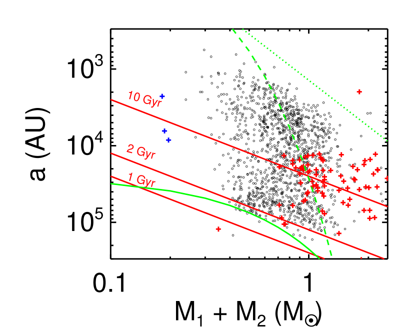
Figure 19.— The physical separation of SLoWPoKES pairs (black circles) and previously known wide CPM doubles (red pluses; Table 4.2) and VLM binaries (blue pluses) as a function of the total mass of the system, as inferred from their $r-z$ colors. Previous studies by Reid et al. (2001a) (green dashed line) and Burgasser et al. (2003) (green dotted line) have also suggested empirical limits for stability. As neither of those describe the SLoWPoKES envelope, we have followed these previous authors and fit a log-normal (solid green line). Numerical simulations by Weinberg et al. (1987) suggest that the lifetime of wide pairs is a function of age as well; the “isochrones” show the expected $a$ vs.  M_tot relationships for dissipation times of 1, 2, and 10 Gyrs (solid red lines), as defined by Eq. (26). While some very wide SLoWPoKES pairs are expected to dissipate on timescales of 1–2 Gyr, most should be stable for $\gtrsim$ 10 Gyrs. All SDs are excluded from this figure.

Interestingly, the widest SLoWPoKES systems appear to violate previously proposed empirical limits on maximum separations (dashed and dotted green lines in Figure 19; Reid et al., 2001a; Burgasser et al., 2003). Similarly, previously proposed empirical limits based on binding energies, $10^{41}$ ergs for stellar and and $10^{42.5}$ ergs very low-mass regimes (Close et al., 2003, 2007; Burgasser et al., 2007), are also violated by SLoWPoKES pairs as well as other known CPM doubles. This is clearly evident in Figure 20, where we see that the most weakly bound SLoWPoKES systems have binding energies of only $\sim 10^{40}$ ergs, comparable to the binding energy of Neptune about the Sun. Faherty et al. (2010) have also noted such transgressions in their sample of wide, very low-mass CPM doubles.

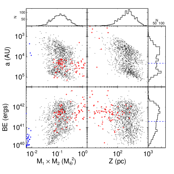
Figure 20.— The physical separations and binding energies of SLoWPoKES pairs as a function of the product of their masses (left) or the Galactic height (right), with the histograms of the distributions shown along the top and the right. For comparison, other CPM pairs (red pluses; Table 4.2) and VLM binaries (blue pluses; VLM binary archive) from the literature are shown. The bimodality in physical separation (at $\sim$0.1 pc) seen in Figures 13 and 19 and along the top panels in this figure is evident in binding energy as well (at $\sim$10^41.3 ergs); these are marked with blue dashed lines in the histograms. As the binding energy is not dependent on $Z$, any selection effects or biases that depend directly or indirectly on $Z$ are not likely to be the cause of the bimodality. Previously suggested minimum binding energy for stellar ($10^{42.5}$ ergs) and substellar ($10^{40}$ ergs) binaries (Close et al., 2003) are violated by most SLoWPoKES as well as other CPM and VLM pairs. All SDs are excluded from this figure.

It seems that previously proposed empirical limits were too restrictive as the widest and the VLM pairs that clearly violate them were not available at the time. We can follow the approach of Reid et al. (2001a) and Burgasser et al. (2003) to fit a log-normal that forms an empirical envelope around the SLoWPoKES pairs (Figure 19, green solid lines). Although this new fit is not likely to define the absolute stability limit for wide pairs, the fit is notable for how well it describes the envelope.

We note that Eq. (26) as well as most previously proposed empirical limits have used the total mass of the system and do not take into account the mass ratio of the components. This creates a degeneracy as the binding energy is dependent on the product of masses. Instead, it may be more physical to consider the wide, low-mass pairs as a function of the product of the masses of their components—i.e., the binding energy (BE) of the system. Figure 20 (left panels) present the $a$ and BE vs. $M_{1}\times M_{2}$ for the SLoWPoKES pairs. That the distribution of $a$ as a function of either sum or product of the component masses appears qualitatively similar is a manifestation of the fact that SLoWPoKES pairs tend to be equal mass (see Figure 14); for high-$q$ pairs there would be a more noticeable difference in these distributions.

Perhaps, of particular interest to the issue of wide binary stability, formation, and evolution is our observation of a distinctly bimodal distribution of binary separations, seen in Figure 20, which equates to a bimodal distribution of system binding energies as well. The break in the bimodal distribution at binding energy $\sim$10^41.3 ergs is remarkable for how well it agrees with the previously proposed empirical limit in binding energy for stellar binaries to be dynamically stable (Close et al., 2003, 2007; Burgasser et al., 2007). In addition, as can be seen in Figure 19, the 10 Gyr disruption “isochrone” of Weinberg et al. (1987) nicely traces the observed break in the distribution over nearly a full decade of total system mass. The trend of the break in the distribution with mass is also important because it makes it very unlikely that the bimodality is the result of observational biases in the SLoWPoKES sample. Similarly, there is no effect of the heliocentric distances or the Galactic heights (Figure 20, right panels) of the pairs on the physical separation or binding energy. As discussed earlier, the principal observational biases in SLoWPoKES affect only (i) the smallest separations most severely because of the strict cut-off at 7$\arcsec$ and (ii) to a lesser extent the largest separations as we limit our search to 180$\arcsec$.

Thus, the bimodal distribution of binary separations suggests two populations of binaries, perhaps representing (i) systems of stars that formed with sufficient binding energy to survive for the age of the Galaxy and (ii) relatively young systems that formed within the past 1–2 Gyr but that will likely not survive much longer. Figure 21 shows that the dispersion in the tangential velocity is indeed smaller for the “young” population, relative to the “old” population that has had more time to get kinematically heated. Quantitatively, the median absolute deviations for the two populations are 46.1  km s^-1 and 32.7  km s^-1. Curiously, the separations of the binaries in the second group (up to 1 pc; Figure 13, right panel) is larger than the typical sizes of prestellar cores ($\sim$0.35 pc), suggesting that these systems may not have formed via the “standard” collapse and fragmentation of individual cloud cores.

Figure 21.— The tangential velocity ($v_{t}=4.74~{}\mu~{}d$) distribution for the low-binding energy population (dashed histogram) and high-binding energy distribution (solid histogram), with the segregation at binding energy of $10^{41.3}$ ergs that was noticed in Figure 20. A smaller dispersion in the tangential velocity supports our suggestion that the low-binding energy distribution is of a younger population.

Recent N-body simulations predict bimodal distributions of wide binary separations and may provide important theoretical insight for understanding the formation and evolution of wide pairs. Although the specific simulations predict bimodality on different scales than seen in our observations, some of the resulting predicted physical properties of pairs are similar to those found in SLoWPoKES. For example, Kouwenhoven et al. (2010) find that the distribution of binary semi-major axes will in general be bimodal on the size scale of star-forming clusters (i.e. $\sim 0.1$ pc), with a group of tight systems formed primarily via dynamical interactions near the cluster center and a second group of loosely bound systems formed through random pairing during the slow dissolution of the cluster. In their simulations, up to $\sim 30$% of the resulting binaries will be in the latter “dissolution peak”, with separations of $\sim 0.1$ pc. They predict that the mass ratios of these systems will reflect random pairing. Alternatively, Jiang & Tremaine (2009) have found that a bimodal distribution arises due to the slow (as opposed to instantaneous), diffusive disruption of systems on timescales of several Gyrs, and that the details of the resulting bimodality is mostly independent of the initial distribution of separations arising from the formation process. Their simulations predict that the bimodal break in the distribution occurs at a few Jacobi radii, which corresponds to a separation of $\sim 2$ pc for a total system of 1 M_⊙. Perhaps the diffusive dissipation mechanism is more efficient than predicted by Jiang & Tremaine (2009), or perhaps the “tidal-tail peak” of dissolving systems has not yet been observed. In the future, the SLoWPoKES catalog can be extended to even larger physical separations to probe this possibility.

6. Conclusions

We have created the SLoWPoKES catalog, comprising 1342 CPM binary pairs, identified through statistical matching of angular separation, photometric distances, and proper motion components. We have sifted the sample of chance alignments using a Galactic model based on empirical observations of stellar spatial and kinematic distributions. With the objective that each pair can be confidently used to investigate various science questions regarding low-mass stars, we have adopted a very restrictive set of selection criteria. This approach clearly underestimates the number of binary systems. Moreover, the sample includes several biases, the most important of which are a lack of systems with physical separations smaller than $\sim 1000$ AU (arising from a strict bias against angular separations smaller than 7$\arcsec$), and the exclusion of certain types of higher-order multiples (e.g. triples) due to the strict photometric distance matching. However, as a consequence the catalog should contain very few false positives, making follow-up studies efficient.

We built a Monte Carlo-based six-dimensional Galactic model that is able to replicate the positional and kinematic properties of the stars in the Milky Way. In its current incarnation, we used it to calculate the the number of stars within a certain spatial volume in the Galaxy and the likelihood that those stars have common kinematics (proper motions) by chance. One of the things this model underscores is how difficult it is to find two physically unassociated stars close together in space: along a typical SDSS LOS, there are expected to be only 0.52 chance alignments within 15$\arcsec$ and a minuscule 0.03 chance alignments if the volume is considered. The additional matching of proper motions gives each of the accepted SLoWPoKES binaries a very low probability of being a false positive.

Due to their intrinsic faintness and the resulting small numbers, binarity studies of low-mass stars have been limited in scope. However, with the advent of large-scale deep surveys, detailed and statistically significant studies of M (and L) dwarfs are being done. SLoWPoKES is now the largest sample to date of very wide, low-mass binaries. In particular, SLoWPoKES provides a large sample of systems with physical separations up to $a\sim$ 1 pc that will be useful for putting firm constraints on the maximum size of physically associated systems. How the widest of these systems form, and how long they survive, is in particular an interesting question that SLoWPoKES is well suited to address. While numerical calculations suggest that approximately half of SLoWPoKES systems can remain bound for at least 10 Gyr (Weinberg et al., 1987), previously proposed empirical limits are violated by many SLoWPoKES systems.

Indeed, the distribution of SLoWPoKES binary separations is distinctly bimodal, suggesting the presence of (i) a population of tightly bound systems formed with sufficient binding energy to remain intact for the age of the Galaxy and (ii) a population of weakly bound systems that recently formed and that are unlikely to survive past 1–2 Gyr. Recent N-body simulations (e.g. Kouwenhoven et al., 2010; Jiang & Tremaine, 2009) in fact predict a bimodal distribution of binary separations on the scales probed by the widest SLoWPoKES systems.

We observed a wide binary frequency of $\sim$1.1%, which is likely to be a minimum given the nature of our sample. While this is consistent with the results from SIJ08 who found 0.9% of stars at $Z=$ 500 pc had wide companions., it is significantly lower than $\sim$9.5% of nearby solar-type Hipparcos stars having wide companions (Lépine & Bongiorno, 2007). While the incompleteness involved in the searching for companions at large distances probably causes some of this, both this study and SIJ08 saw a decrease in binary fraction as a function of Galactic height, evidence of dynamical destruction of older systems. Hence, the wide binary fraction around our initial sample of low-mass stars might actually be significantly lower than the Hipparcos stars.

Besides the importance of SLoWPoKES for constraining models of formation and evolution of binary stars, SLoWPoKES systems are coeval laboratories—sharing an identical formation and evolutionary history without affecting each other—making them ideal for measuring and calibrating empirical relationships between rotation, activity, metallicity, age, etc. We have started programs to test and calibrate the age–activity relationship measured by West et al. (2008) and to explore whether gyrochronology (Barnes, 2003, 2007) can be applied in the fully-convective regime. As coeval laboratories allow for the removal of one or more of the three fundamental parameters (mass, age, and metallicity), much more science can be done with a large sample of such systems.

Future astrometric missions, such as the Space Interferometry Mission (SIM), should provide exquisite astrometry, perhaps enabling us to trace the orbits of some of the SLoWPoKES systems. While tracing orbits with periods $\gtrsim 10^{4-6}$ years sounds ambitious, with SIM’s microarcsecond level (or better) astrometry (Unwin et al., 2008) combined with SDSS, DSS, and/or other epochs, it is not unrealistic. Similarly, the “identical” twins in SLoWPoKES would be ideal sites to probe for the presence and differences in the formation mechanism of planets. As each identical twin in a CPM double provides similar environment for the formation and evolution of planets, these systems can be ideal sites to study planetary statistics. Due to their large separations the stars are not expected to influence each others evolution but have similar mass, age, and metallicity, as we noted earlier in § 1.

The SLoWPoKES catalog, as the name suggests, only contains systems for which kinematic information is available. We can, however, use the results from the Galactic model to identify pairs at the small separations ($\Delta\theta<7\arcsec$), albeit with a larger uncertainty, for which no kinematic information is available. Similarly companions which are fainter than $r=$ 20 can also be identified as the SDSS photometry is complete to $r=$ 22.5. The latter systems are likely to be skewed towards late-type dMs and unequal-mass pairs. A follow-up paper will study such systems and will add a large proportion of wide systems.

References

- Abazajian et al. (2009) Abazajian, K. N., et al. 2009, ApJS, 182, 543
- Abt & Levy (1976) Abt, H. A., & Levy, S. G. 1976, ApJS, 30, 273
- Adelman-McCarthy et al. (2008) Adelman-McCarthy, J. K., et al. 2008, ApJS, 175, 297
- Allen et al. (2000) Allen, C., Poveda, A., & Herrera, M. A. 2000, A&A, 356, 529
- Artigau et al. (2009) Artigau, É., Lafrenière, D., Albert, L., & Doyon, R. 2009, ApJ, 692, 149
- Artigau et al. (2007) Artigau, É., Lafrenière, D., Doyon, R., Albert, L., Nadeau, D., & Robert, J. 2007, ApJ, 659, L49
- Bahcall et al. (1985) Bahcall, J. N., Hut, P., & Tremaine, S. 1985, ApJ, 290, 15
- Bahcall & Soneira (1980) Bahcall, J. N., & Soneira, R. M. 1980, ApJS, 44, 73
- Bahcall & Soneira (1981) ——. 1981, ApJ, 246, 122
- Barnes (2003) Barnes, S. A. 2003, ApJ, 586, 464
- Barnes (2007) ——. 2007, ApJ, 669, 1167
- Benson & Myers (1989) Benson, P. J., & Myers, P. C. 1989, ApJS, 71, 89
- Bergeron et al. (1995) Bergeron, P., Wesemael, F., & Beauchamp, A. 1995, PASP, 107, 1047
- Bochanski et al. (2010) Bochanski, J. J., Hawley, S. L., Covey, K. L., Reid, I. N., West, A. A., Golimowski, D. A., & Izezic, A. 2010, AJ, submitted
- Bochanski et al. (2007) Bochanski, J. J., Munn, J. A., Hawley, S. L., West, A. A., Covey, K. R., & Schneider, D. P. 2007, AJ, 134, 2418
- Bond et al. (2009) Bond, N. A., Ivezic, Z., Sesar, B., Juric, M., & Munn, J. 2009, ArXiv e-prints
- Bonfils et al. (2005) Bonfils, X., Delfosse, X., Udry, S., Santos, N. C., Forveille, T., & Ségransan, D. 2005, A&A, 442, 635
- Bouy et al. (2003) Bouy, H., Brandner, W., Martín, E. L., Delfosse, X., Allard, F., & Basri, G. 2003, AJ, 126, 1526
- Burgasser et al. (2003) Burgasser, A. J., Kirkpatrick, J. D., Reid, I. N., Brown, M. E., Miskey, C. L., & Gizis, J. E. 2003, ApJ, 586, 512
- Burgasser et al. (2007) Burgasser, A. J., Reid, I. N., Siegler, N., Close, L., Allen, P., Lowrance, P., & Gizis, J. 2007, in Protostars and Planets V, ed. B. Reipurth, D. Jewitt, & K. Keil, 427–441
- Caballero (2007) Caballero, J. A. 2007, ApJ, 667, 520
- Caballero (2009) ——. 2009, A&A, 507, 251
- Caballero (2010) ——. 2010, ArXiv e-prints
- Carollo et al. (2009) Carollo, D., et al. 2009, ArXiv e-prints
- Carollo et al. (2008) ——. 2008, Nature, 451, 216
- Chanamé & Gould (2004) Chanamé, J., & Gould, A. 2004, ApJ, 601, 289
- Clarke (1992) Clarke, C. 1992, in Astronomical Society of the Pacific Conference Series, Vol. 32, IAU Colloq. 135: Complementary Approaches to Double and Multiple Star Research, ed. H. A. McAlister & W. I. Hartkopf, 176–+
- Clemens et al. (1991) Clemens, D. P., Yun, J. L., & Heyer, M. H. 1991, ApJS, 75, 877
- Close et al. (2003) Close, L. M., Siegler, N., Freed, M., & Biller, B. 2003, ApJ, 587, 407
- Close et al. (2007) Close, L. M., et al. 2007, ApJ, 660, 1492
- Covey et al. (2007) Covey, K. R., et al. 2007, AJ, 134, 2398
- Cutri et al. (2003) Cutri, R. M., et al. 2003, 2MASS All Sky Catalog of point sources. (The IRSA 2MASS All-Sky Point Source Catalog, NASA/IPAC Infrared Science Archive. http://irsa.ipac.caltech.edu/applications/Gator/)
- Delfosse et al. (2004) Delfosse, X., et al. 2004, in ASP Conference Series, Vol. 318, Spectroscopically and Spatially Resolving the Components of the Close Binary Stars, ed. R. W. Hilditch, H. Hensberge, & K. Pavlovski, 166–174
- Duchêne et al. (1999) Duchêne, G., Bouvier, J., & Simon, T. 1999, A&A, 343, 831
- Duquennoy & Mayor (1991) Duquennoy, A., & Mayor, M. 1991, A&A, 248, 485
- Faherty et al. (2009) Faherty, J. K., Burgasser, A. J., Cruz, K. L., Shara, M. M., Walter, F. M., & Gelino, C. R. 2009, AJ, 137, 1
- Faherty et al. (2010) Faherty, J. K., Burgasser, A. J., West, A. A., Bochanski, J. J., Cruz, K. L., Shara, M. M., & Walter, F. M. 2010, AJ, 139, 176
- Fischer & Marcy (1992) Fischer, D. A., & Marcy, G. W. 1992, ApJ, 396, 178
- Fukugita et al. (1996) Fukugita, M., Ichikawa, T., Gunn, J. E., Doi, M., Shimasaku, K., & Schneider, D. P. 1996, AJ, 111, 1748
- Garnavich (1988) Garnavich, P. M. 1988, ApJ, 335, L47
- Ghez et al. (1997) Ghez, A. M., McCarthy, D. W., Patience, J. L., & Beck, T. L. 1997, ApJ, 481, 378
- Gies (1987) Gies, D. R. 1987, ApJS, 64, 545
- Gilmore et al. (1989) Gilmore, G., Wyse, R. F. G., & Kuijken, K. 1989, ARA&A, 27, 555
- Gizis et al. (2003) Gizis, J. E., Reid, I. N., Knapp, G. R., Liebert, J., Kirkpatrick, J. D., Koerner, D. W., & Burgasser, A. J. 2003, AJ, 125, 3302
- Goodwin & Kroupa (2005) Goodwin, S. P., & Kroupa, P. 2005, A&A, 439, 565
- Goodwin et al. (2007) Goodwin, S. P., Kroupa, P., Goodman, A., & Burkert, A. 2007, in Protostars and Planets V, ed. B. Reipurth, D. Jewitt, & K. Keil, 133–147
- Goodwin et al. (2004) Goodwin, S. P., Whitworth, A. P., & Ward-Thompson, D. 2004, A&A, 414, 633
- Gunn et al. (1998) Gunn, J. E., et al. 1998, AJ, 116, 3040
- Halbwachs (1986) Halbwachs, J. L. 1986, A&AS, 66, 131
- Halbwachs et al. (2003) Halbwachs, J. L., Mayor, M., Udry, S., & Arenou, F. 2003, A&A, 397, 159
- Harris et al. (2006) Harris, H. C., et al. 2006, AJ, 131, 571
- Heintz (1969) Heintz, W. D. 1969, JRASC, 63, 275
- Henry et al. (1999) Henry, T. J., Franz, O. G., Wasserman, L. H., Benedict, G. F., Shelus, P. J., Ianna, P. A., Kirkpatrick, J. D., & McCarthy, Jr., D. W. 1999, ApJ, 512, 864
- Henry & McCarthy (1993) Henry, T. J., & McCarthy, Jr., D. W. 1993, AJ, 106, 773
- Ivezić et al. (2008) Ivezić, Ž., et al. 2008, ApJ, 684, 287
- Jessop & Ward-Thompson (2000) Jessop, N. E., & Ward-Thompson, D. 2000, MNRAS, 311, 63
- Jiang & Tremaine (2009) Jiang, Y., & Tremaine, S. 2009, MNRAS, 1640
- Johnson & Soderblom (1987) Johnson, D. R. H., & Soderblom, D. R. 1987, AJ, 93, 864
- Jurić et al. (2008) Jurić, M., et al. 2008, ApJ, 673, 864
- Kenyon & Hartmann (1995) Kenyon, S. J., & Hartmann, L. 1995, ApJS, 101, 117
- Kilic et al. (2006) Kilic, M., et al. 2006, AJ, 131, 582
- Kohler & Leinert (1998) Kohler, R., & Leinert, C. 1998, A&A, 331, 977
- Kouwenhoven et al. (2010) Kouwenhoven, M. B. N., Goodwin, S. P., Parker, R. J., Davies, M. B., Malmberg, D., & Kroupa, P. 2010, ArXiv e-prints
- Kraus & Hillenbrand (2007) Kraus, A. L., & Hillenbrand, L. A. 2007, AJ, 134, 2340
- Kraus & Hillenbrand (2009) ——. 2009, ApJ, 703, 1511
- Latham et al. (1984) Latham, D. W., Schechter, P., Tonry, J., Bahcall, J. N., & Soneira, R. M. 1984, ApJ, 281, L41
- Laughlin et al. (1997) Laughlin, G., Bodenheimer, P., & Adams, F. C. 1997, ApJ, 482, 420
- Lawrence et al. (2007) Lawrence, A., et al. 2007, MNRAS, 379, 1599
- Leinert et al. (1993) Leinert, C., Zinnecker, H., Weitzel, N., Christou, J., Ridgway, S. T., Jameson, R., Haas, M., & Lenzen, R. 1993, A&A, 278, 129
- Lépine & Bongiorno (2007) Lépine, S., & Bongiorno, B. 2007, AJ, 133, 889
- Lépine et al. (2007) Lépine, S., Rich, R. M., & Shara, M. M. 2007, ApJ, 669, 1235
- Lépine & Scholz (2008) Lépine, S., & Scholz, R.-D. 2008, ApJ, 681, L33
- Lépine & Shara (2005) Lépine, S., & Shara, M. M. 2005, AJ, 129, 1483
- Longhitano & Binggeli (2010) Longhitano, M., & Binggeli, B. 2010, ArXiv e-prints
- Luyten (1922) Luyten, W. J. 1922, Lick Observatory Bulletin, 10, 135
- Luyten (1979) ——. 1979, LHS catalogue. A catalogue of stars with proper motions exceeding 0”5 annually (Minneapolis: University of Minnesota, 1979, 2nd ed.)
- Luyten (1988) ——. 1988, Ap&SS, 142, 17
- Majewski (1993) Majewski, S. R. 1993, ARA&A, 31, 575
- Makarov et al. (2008) Makarov, V. V., Zacharias, N., & Hennessy, G. S. 2008, ApJ, 687, 566
- Martín et al. (2003) Martín, E. L., Barrado y Navascués, D., Baraffe, I., Bouy, H., & Dahm, S. 2003, ApJ, 594, 525
- Mason et al. (1998) Mason, B. D., Gies, D. R., Hartkopf, W. I., Bagnuolo, Jr., W. G., ten Brummelaar, T., & McAlister, H. A. 1998, AJ, 115, 821
- Mason et al. (2009) Mason, B. D., Hartkopf, W. I., Gies, D. R., Henry, T. J., & Helsel, J. W. 2009, AJ, 137, 3358
- Miller & Scalo (1979) Miller, G. E., & Scalo, J. M. 1979, ApJS, 41, 513
- Munn et al. (2004) Munn, J. A., et al. 2004, AJ, 127, 3034
- Munn et al. (2008) ——. 2008, AJ, 136, 895
- Petr et al. (1998) Petr, M. G., Coude Du Foresto, V., Beckwith, S. V. W., Richichi, A., & McCaughrean, M. J. 1998, ApJ, 500, 825
- Pier et al. (2003) Pier, J. R., Munn, J. A., Hindsley, R. B., Hennessy, G. S., Kent, S. M., Lupton, R. H., & Ivezić, Ž. 2003, AJ, 125, 1559
- Poveda et al. (2009) Poveda, A., Allen, C., Costero, R., Echevarría, J., & Hernández-Alcántara, A. 2009, ApJ, 706, 343
- Press et al. (1992) Press, W. H., Teukolsky, S. A., Vetterling, W. T., & Flannery, B. P. 1992, Numerical recipes in FORTRAN. The art of scientific computing (Cambridge: University Press, —c1992, 2nd ed.)
- Quinn et al. (2009) Quinn, D. P., Wilkinson, M. I., Irwin, M. J., Marshall, J., Koch, A., & Belokurov, V. 2009, MNRAS, 396, L11
- Radigan et al. (2008) Radigan, J., Lafrenière, D., Jayawardhana, R., & Doyon, R. 2008, ApJ, 689, 471
- Radigan et al. (2009) ——. 2009, ApJ, 698, 405
- Reid & Gizis (1997) Reid, I. N., & Gizis, J. E. 1997, AJ, 113, 2246
- Reid et al. (2001a) Reid, I. N., Gizis, J. E., Kirkpatrick, J. D., & Koerner, D. W. 2001a, AJ, 121, 489
- Reid et al. (2002) Reid, I. N., Kirkpatrick, J. D., Liebert, J., Gizis, J. E., Dahn, C. C., & Monet, D. G. 2002, AJ, 124, 519
- Reid et al. (2001b) Reid, I. N., van Wyk, F., Marang, F., Roberts, G., Kilkenny, D., & Mahoney, S. 2001b, MNRAS, 325, 931
- Reid (1998) Reid, N. 1998, AJ, 115, 204
- Salim & Gould (2003) Salim, S., & Gould, A. 2003, ApJ, 582, 1011
- Schmidt et al. (2010) Schmidt, S. J., West, A. A., Hawley, S. L., & Pineda, J. S. 2010, ArXiv e-prints
- Sesar et al. (2008) Sesar, B., Ivezić, Ž., & Jurić, M. 2008, ApJ, 689, 1244
- Silvestri et al. (2005) Silvestri, N. M., Hawley, S. L., & Oswalt, T. D. 2005, AJ, 129, 2428
- Simon et al. (1999) Simon, M., Close, L. M., & Beck, T. L. 1999, AJ, 117, 1375
- Stassun et al. (2008) Stassun, K. G., Mathieu, R. D., Cargile, P. A., Aarnio, A. N., Stempels, E., & Geller, A. 2008, Nature, 453, 1079
- Stassun et al. (2007) Stassun, K. G., Mathieu, R. D., & Valenti, J. A. 2007, ApJ, 664, 1154
- Unwin et al. (2008) Unwin, S. C., et al. 2008, PASP, 120, 38
- Wasserman & Weinberg (1991) Wasserman, I., & Weinberg, M. D. 1991, ApJ, 382, 149
- Weinberg et al. (1987) Weinberg, M. D., Shapiro, S. L., & Wasserman, I. 1987, ApJ, 312, 367
- West et al. (2008) West, A. A., Hawley, S. L., Bochanski, J. J., Covey, K. R., Reid, I. N., Dhital, S., Hilton, E. J., & Masuda, M. 2008, AJ, 135, 785
- West et al. (2004) West, A. A., et al. 2004, AJ, 128, 426
- West et al. (2005) West, A. A., Walkowicz, L. M., & Hawley, S. L. 2005, PASP, 117, 706
- White & Ghez (2001) White, R. J., & Ghez, A. M. 2001, ApJ, 556, 265
- White et al. (1999) White, R. J., Ghez, A. M., Reid, I. N., & Schultz, G. 1999, ApJ, 520, 811
- Woolf & Wallerstein (2005) Woolf, V. M., & Wallerstein, G. 2005, MNRAS, 356, 963
- Yoo et al. (2004) Yoo, J., Chanamé, J., & Gould, A. 2004, ApJ, 601, 311
- York et al. (2000) York, D. G., et al. 2000, AJ, 120, 1579
- Zapatero Osorio & Martín (2004) Zapatero Osorio, M. R., & Martín, E. L. 2004, A&A, 419, 167