The stellar mass fraction and baryon content of galaxy clusters and groups

Abstract

The analysis of a sample of 52 clusters with precise and hypothesis-parsimonious measurements of mass, derived from caustics based on about 208 member velocities per cluster on average, shows that low mass clusters and groups are not simple scaled-down versions of their massive cousins in terms of stellar content: lighter clusters have more stars per unit cluster mass. The same analysis also shows that the stellar content of clusters and groups displays an intrinsic spread at a given cluster mass, i.e. clusters are not similar each other in the amount of stars they contain, not even at a fixed cluster mass. The stellar mass fraction depends on halo mass with (logarithmic) slope $-0.55\pm 0.08$ and with $0.15\pm 0.02$ dex of intrinsic scatter at a fixed cluster mass. These results are confirmed by adopting masses derived from velocity dispersion. The intrinsic scatter at a fixed cluster mass we determine for gas mass fractions taken from literature is smaller, $0.06\pm 0.01$ dex. The intrinsic scatter in both the stellar and gas mass fractions is a distinctive signature that, when taken individually, the regions from which clusters and groups collected matter, a few tens of Mpc, are yet not representative, in terms of gas and baryon content, of the mean matter content of the Universe. The observed stellar mass fraction values are in marked disagreement with gasdynamics simulations with cooling and star formation of clusters and groups. Instead, amplitude and cluster mass dependency of observed stellar mass fractions are those requested not to need any AGN feedback to describe gas and stellar mass fractions and X-ray scale relations in simple semi-analytic cluster models. By adding stellar and gas masses and accounting for the intrinsic variance of both quantities, we found the the baryon fraction is fairly constant for clusters and groups with masses between $10^{13.7}$ and $10^{15.0}$ solar masses and it is offset from the WMAP-derived value by about 6 sigmas. The offset is unlikely to be due to an underestimate of the stellar mass fraction, and could be related to the possible non universality of the baryon fraction, pointed out by our measurements of the intrinsic scatter. Our analysis is the first that does not assume that clusters are identically equal at a given halo mass and it is also more accurate in many aspects. The data and code used for the stochastic computation are distributed with the paper.

1 Introduction

Knowledge of the baryon content of clusters and groups is a key ingredient in our understanding of the physics of these objects and in their use as cosmological probes. In fact, clusters have accreted matter from a region of some tens of Mpc, large enough that their content should be representative of the mean matter content of the Universe (White et al. 1993). If this is the case, by measuring the baryon fraction in clusters, $f_{b}$, and coupling it with an estimate of $\Omega_{b}$, for example from primordial nucleosynthesis arguments or from CMB anisotropies, gives $\Omega_{m}=\Omega_{b}\ f_{b}$ (e.g. White et al. 1993; Evrard et al. 1997). Second, the study of how baryons are distributed in gas and stars and the way this splitting depends on halo (cluster or group) mass, should provide clues to the role played by the various physical mechanisms potentially active in clusters and groups.

However, the baryon fraction is far from being fully understood: WMAP-derived value of the baryon fraction is larger than all values found in X-ray analysis (i.e. Vikhlinin et al. 2006) even accounting for baryons in stars (e.g. Gonzalez, Zaritsky, & Zabludoff 2007), and gas depletion (e.g. Nagai et al. 2007). X-ray scaling relations (e.g. halo mass vs Temperature or X-ray luminosity) predicted on the assumption that the thermal energy of the gas comes solely from the gravitational collapse are notoriously in disagreement with observed scalings (e.g. Vikhlinin et al. 2006). Observed and predicted scalings may be bring in agreement by allowing star formation, and, eventually a further feedback (e.g. Kravsov et al. 2005, Nagai, Kravtsov, & Vikhlinin 2007; Bode et al. 2009; Fabjan et al. 2009). In particular, whether a further feedback, i.e. in addition to the stellar one, is needed, is largely unknown because of the uncertainty of the observed stellar mass content of clusters (e.g. Bode et al. 2009). More generally, recent works on the subject achieve to reproduce X-ray derived quantities (e.g. baryon fraction or mass-temperature scaling relations) by basically adding to the cluster model a further degree of freedom associated with star formation (e.g. Nagai, Kravtsov, & Vikhlinin 2007; Bode et al. 2009; Fabjan et al. 2009), without adding the corresponding observational constraint, i.e. requiring that the stellar mass produced in the model fit the data. We emphasise that gas properties strongly depend on the amount of stellar mass allowed in the model (e.g. Nagai & Kravtsov 2005; Kravtsov et al. 2005; Nagai, Kravtsov & Vikhlinin 2007) and a constraint on the stellar component has a direct and important consequence on the gas component of the model.

Several observational determinations of the stellar mass fraction suffer by important limitations: published works studied clusters with unmeasured, or very poorly measured, masses and unmeasured reference radii, while these quantities are requested to be known for the determination of the stellar mass fraction, as discussed in later sections. It is clear, therefore, that an observational measurement of the stellar mass fraction of clusters with known masses and reference radii is valuable.

The caustic method (Diaferio & Geller 1997; Diaferio 1999) offers a robust path to estimating cluster mass and reference radii. It relies on the identification in projected phase-space (i.e. in the plane of line-of-sight velocities and projected cluster-centric radii, $v,R$) of the envelope defining sharp density contrasts (i.e. caustics) between the cluster and the field region. The amplitude of such an envelope is a measure of the mass inside $R$. As opposed to masses derived in other ways (e.g. from X-ray, from velocity dispersion, from the virial theorem, from the Jeans method, etc.) caustic masses do not require that the cluster is in dynamical equilibrium (see Rines & Diaferio 2006 for a discussion). There is a good agreement between caustic and lensing masses for the very few clusters where both measurements are available (Diaferio, Geller, & Rines 2005). On larger cluster samples, caustic masses also shows a good agreement with virial masses (e.g. Rines & Diaferio 2006, Andreon & Hurn 2010) and with the extrapolation to larger radii of dynamical masses derived through a Jean analysis (Biviano & Girardi 2003). Both virial and Jean masses require, however, assume that the cluster is in dynamical equilibrium.

This paper addresses: a) the determination of the stellar mass fraction in a sample of clusters and groups with well determined masses and reference radii derived by the caustic method, using, on average, 208 members per cluster; and b) the determination of the average baryon content of clusters and groups.

Throughout this paper we assume $\Omega_{M}=0.3$, $\Omega_{\Lambda}=0.7$ and $H_{0}=70$ km s^-1 Mpc^-1. Magnitudes are quoted in their native system (quasi-AB for SDSS magnitudes).

2 Data & Sample

The final cluster (halo) sample consist of the 52 clusters and groups with accurate caustic masses (Rines & Diaferio 2006) fully included in the Sloan Digital Sky Survey (hereafter SDSS) $6^{th}$ data release (Adelman-McCarthy et al., 2008). Fundamentally, clusters/groups are: a) X-ray flux-selected b) with an upper cut at redshift $z=0.1$ (to allow a good caustic measurement). From the original Rines & Diaferio (2006) larger sample, we removed (in Andreon & Hurn 2010) only clusters at $z<0.03$ to avoid shredding problems (large galaxies are split in many smaller sources), two cluster pairs (requiring a deblending algorithm), and one further cluster, the NGC4325 group, because is of very low richness. In the present paper, one more group, MKW11, has been removed because the star/galaxy classification of SDSS is poor at this cluster location, as verified by visual inspection (see Sec 3.2). It turned out also that MKW11 is the halo with smallest mass in our sample.

We emphasise that only two cluster pairs have been removed from the original sample because of their morphology, all the other excluded clusters have been removed because they are not fully enclosed in the sky area observed by SDSS, or have bad SDSS data, or have suspect masses because the algorithm used to compute the caustic mass converged on a secondary galaxy clump.

The basic data used in our analysis are $g$ and $r$ photometry from SDSS, down to $r=19$ mag. The latter value is the value where the star/galaxy separation becomes uncertain (e.g. Lupton et al. 2002) and is well brighter than the SDSS completeness limit (e.g. Ivezić et al. 2002). Specifically, we use petrosian magnitudes for “total” magnitudes, and “dered” magnitudes for colours.

3 Analysis of the individual clusters

We want to measure the stellar mass fraction and its dependence on cluster mass. To do this, we must a) measure cluster masses and determine reference radii, b) determine the total luminosity in galaxies, c) estimate the luminosity of other components (e.g., the brightest cluster galaxy and intracluster light), and d) convert the stellar luminosity into stellar mass. In addition to the above, when the total baryon content is of interest, we also need the gas mass fraction.

About point a), we adopted virial masses, $M200$, and virial radii, $r_{200}$, from the caustic analysis of Rines & Diaferio (2006). For sake of precision, $r_{200}$ is the radius within which the enclosed average mass density is $200$ times the critical density. Let’s consider the remaining points in turn.

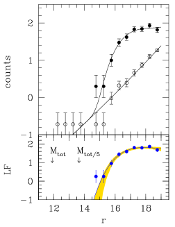
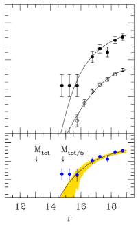
Figure 1: LF determination. The figure shows galaxy counts in the cluster direction (upper panel, solid dots), in a reference line of sight (upper panel, open dots), and the cluster luminosity function (bottom panel). Curves mark the fitted model to un-binned data. Approximated errors (computed with the usual sum in quadrature) are marked with bars, precisely computed errors are shaded. The bottom panel also reports the integral of the luminosity function ($M_{tot}$) and $1/5^{th}$ of it ($M_{tot/5}$), useful to note the presence of a bright galaxy or a mis-classified star. The left/right panel refers to the cluster with the third best/worst stellar mass determination (Zw1215.1+0400/Abell 954).

3.1 Luminosity function and its integral

In order to measure the stellar mass of galaxies, we restrict our attention to red galaxies only: blue galaxies would increase little the stellar mass (e.g. Fukugita et al. 1998). In fact: a) blue galaxies have lower mass at a given luminosity in observations (e.g. Hoekstra et al. 2005) and in stellar population synthesis models (e.g. Bruzual & Charlot 2003); and b) blue galaxies are, on average, fainter than red galaxies and less abundant in clusters. Therefore their contribution to the total mass is negligible (e.g. Fukugita et al. 1998; Girardi et al. 2000) and thus neglected. Nevertheless, confirmation of the small role played by blue galaxies in the total stellar mass budget, perhaps derived from a better mass tracer such as near–infrared photometry, would be valuable especially for less massive clusters where their contribution is potentially higher in percentage.

In this paper we define red galaxies those within 0.1 redward and 0.2 blueward in $g-r$ of the colour–magnitude relation, precisely as in Andreon & Hurn (2010), and in agreement with works there mentioned. For the colour center, we took the peak of the colour distribution. For the slope, we adopted the best fit value derived for the richest clusters. This definition of “red” is quite simple because for our cluster sample results hardly depends on the details of the “red” definition: the determination of the precise location of the colour–magnitude relation is irrelevant because the latter is much narrower than the adopted 0.3 mag width and because practically all galaxies brighter than the adopted luminosity cut are red. Colours are corrected for the colour–magnitude slope, but the precise slope determination is not critical given the reduced magnitude range explored (less than $\pm 3$ magnitudes) and the shallow slope of colour–magnitude relation.

The luminosity function is computed in two different ways: for display purposes only we bin galaxies in magnitude bins and we account for the background (galaxies in the cluster line of sight) computing the difference of counts in the cluster and a reference line of sight (e.g. Zwicky 1957, Oemler 1974, and many papers since them), the latter taken outside the cluster turnaround radius or near to it for clusters near the SDSS sky boundaries. For display purpose only, errors are computed with the usual quadrature sum rule. For our formal analysis, instead, we take a Bayesian approach as done for other clusters (e.g. Andreon 2006, Andreon et al. 2006, 2008b, etc): we use the likelihood given in Andreon, Punzi & Grado (2005), which is the extension of the Sandage, Tammann, Yahil (1979) likelihood to the case when a background is present. We fit each cluster, independently on the other ones and without binning data in magnitude bins. We adopt uniform priors for all parameters, and we note that any other weak prior would have returned a similar result because parameters are well determined by the data. For the same reason, a maximum likelihood analysis, such as the one advocated in Andreon, Punzi & Grado (2005), would have returned identical values for the parameters (but with different meanings). However, the Bayesian approach has a number of advantages, amongst which it makes trivial to compute uncertainties on derived parameters, as the error on the integral of the luminosity function (that we need in order to estimate the stellar mass fraction), fully accounting for the covariance of all error terms and with just one line of code (by typing the about 20 characters in eq. 1 below). As usual, all magnitudes are internally zero-pointed to a number near to the average, because this has a number of numerical advantages.

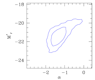
Figure 2: Characteristic magnitude $M^{*}_{r}$ vs faint end slope $\alpha$ of Abell 954. There is a clear covariance between these two Schechter parameters. 68 % and 95 % credible contours are plotted.

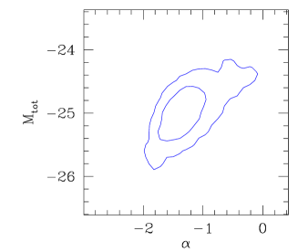
Figure 3: Integral of the LF, $M_{tot}$ vs $\alpha$ of Abell 954. 68 % and 95 % credible contours are plotted.

Figure 1 exemplifies our analysis for two clusters, chosen as those having the third best and worst determination of the stellar mass: top panels show galaxy counts in the cluster (solid dots) and reference (open dots) line of sigh. The cluster contribution is the excess over the reference line of sight. The background is modeled with a $2^{nd}$ degree power law, the cluster with a Schechter (1976) function with the usual parameters $\alpha$ (faint-end slope), $\phi^{*}$ (normalization) and $M^{*}$ (characteristic magnitude). The lines show the fitted model on un-binned data. The bottom panel shows the cluster LF as classically derived (points with the mentioned heuristic error bars) and its Bayesian derivation (mean model with 68 % confidence bounds on it, shaded in yellow).

The analysis is repeated for all 52 (plus one, later discarded) studied clusters.

The total luminosity is given by the integral of the luminosity function, that, for a Schechter (1976) function is given by:

$$L_{tot}=\phi^{*}L^{*}\Gamma(\alpha+2)$$ (1)

Figure 2 and 3 show the $M^{\star}_{r}$ vs $\alpha$ and $M_{tot}$ vs $\alpha$ of the cluster Abell 954. These figures clarify a number of technical aspects. First, there is a covariance between these quantities. Second, as shown for Abell 954 from the comparison of Figures 2 and 3, the error on $M_{tot}$ is smaller than the quadrature sum of its parts, and even on $M^{*}_{r}$ error alone, owing the covariance between variables. For our sample of 52 clusters, the average $M^{*}_{r}$ error is 0.45 mag and the average $M_{tot}$ error is 0.21 mag. Third, if, following almost all previous literature works (e.g. Lin et al. 2003; Gonzalez et al. 2007; Giodini et al. 2009, etc.), a single value of $\alpha$ is instead taken (justifying the above by stating that $\alpha$ is undertermined from the available data), then the derived error would underestimate the true error on $M_{tot}$ (and even more so the one of $M^{*}$). In fact, what literature works measure is the vertical thickness at a given $\alpha$, instead than the overall width, obtained by projecting the likelihood (posterior) on on the $y$ axis (i.e. marginalizing on $\alpha$).

The luminosity we derived thus far is the one emitted from cluster galaxies in a cylinder of radius $r_{200}$. To compute the stellar mass faction we need instead the luminosity within a sphere, the latter derived from the luminosity in a cylinder assuming a Navarro, Frank & White (1997) distribution with concentration equal to 3. If, instead, the true value of the concentration would be 5, then we would be under-estimating stellar masses by 0.02 dex, a negligible quantity compared to the final stellar mass uncertainty (0.08 dex, on average, Sec. 3.4).

3.2 The bright and faint ends

The lower panel of Figure 1 is very useful to detect the presence of galaxies that might give a large contribution to the total cluster flux, like the brightest cluster galaxy (BCG, hereafter) but also bright galaxies unrelated with the cluster or mis-classified bright stars. Every galaxy near to, or brighter than, $1/5^{th}$ of the total cluster flux has been carefully checked. Furthermore, several fainter galaxies, down to the magnitude where the (preliminary computed) LF predicts less than one galaxy, were also checked. First of all, we inspected the SDSS image, and we sometime found that the checked galaxy is instead a misclassified and saturated star. In such case, the object is removed from the sample. In such a check, we noted that the SDSS star/galaxy classification is poor at the location of the cluster MKW11 (there are many stars misclassified as galaxies), which has been removed from the sample. Then, we checked if the candidate BCG is a cluster member or a foreground galaxy by searching its redshift in the SDSS and NED archives and comparing it to the cluster redshift. We either found that the checked galaxy has a fairly different redshift ($\Delta v>4000$ km/s) and, in that case, we removed it from the sample, or very near to it (less than few hundreds km/s) and we kept it in the sample. At this point we have six BCGs much brighter than the LF, all spectroscopically confirmed as cluster member. We now consider the possibility that BGCs are not drawn from the Schechter (1976) function, at the light of several literature claims that BCGs may be drawn from a different distribution (e.g. Tremaine & Richstone 1977). In order to caution us against the risk of missing this source of stellar mass, we (temporary) remove the object from the sample, or better, we remove a magnitude range largely including the BCG, and we re-compute the LF rigorously accounting for missing luminosity range (censored and truncated observations, e.g. in Andreon, Punzi & Grado 2005). We re-integrate the model LF over the full luminosity range, and we add back the temporary removed BCG flux. We find that the median flux of the six BCGs is 16 per cent of the cluster flux.

It is well known that shallow photometric data miss the flux coming from the galaxy outer regions (e.g. Andreon 2002), or, equivalently, that Petrosian magnitudes listed in the SDSS catalog underestimate the total galaxy flux (e.g. Blanton et al. 2001). For de Vaucouleurs (1948) profiles, typical of red galaxies of interest here, Petrosian magnitudes underestimate the total flux by about 15 % (Blanton et al. 2001) for galaxies with the size of those studied in this paper. Our total flux is corrected for this missed flux.

There is one more component to be accounted for, the intracluster light. Of course, it should be counted only once in our measurement of the total flux. Therefore, its value should not include the light coming from the galaxy outer halos, from the BCG, and from faint galaxies (e.g. too faint to be individually detected) because we already accounted for these three terms. Zibetti et al. (2005) measure it by accounting for the three mentioned terms on a stack of clusters and found a small (10 % within 500 kpc, about $r_{200}/2$ for their clusters) and decreasing fraction with clustercentric radii. At the radius of interest, $r_{200}$, it is a minor term, and therefore it is neglected. The small spatial extent of the ICL is confirmed by the Gonzalez et al. (2007) analysis: 80 % of the BCG+ICL total light is contained in the inner 300 kpc.

We can independently confirm the smallness of the ICL luminosity using measurements from Gonzalez et al. (2007), after accounting for different definitions of ICL among works. These authors measured the intracluster+BCG light and found that 30 % of the total light is in the intracluster+BCG light at $r_{200}$. These authors studied clusters that contain a dominant BCG. We estimate the contribution of the BCG light in Gonzalez et al. (2007) sample as similar to the one in clusters dominated by a BCG in our own sample, about 16 %. Gonzalez et al. (2007) quote that a few more per cent of the faint galaxy flux, we counted with LF, ends up in the their BCG+ICL measurement, and we comment that some few more per cent of the flux from the galaxy halo also likely ends up in the their BCG+ICL measurement. In summary, the ICL, defined as in our own paper, measured by Gonzalez et al. (2007) is 10 % with large errors, because of the indirect path used to infer it. This estimate confirms the measurement performed by Zibetti et al. (2005): the ICL (as defined in our own and Zibetti et al. 2005 paper) contribution is negligible at $r_{200}$. We emphasize that some other papers uses the term “cD halo” to indicate the flux that is counted with/as “intracluster light”.

Table 1: Stellar masses and errors

id	$\log M_{\star}$	id	$\log M_{\star}$
	[$M_{\odot}$]		[$M_{\odot}$]
A0160	$12.41\pm 0.10$	A1728	$12.52\pm 0.09$
A0602	$12.49\pm 0.09$	RXJ1326.2+0013	$12.27\pm 0.13$
A0671	$12.74\pm 0.08$	A1750	$12.84\pm 0.07$
A0779	$12.32\pm 0.09$	A1767	$12.87\pm 0.06$
A0957	$12.46\pm 0.09$	A1773	$12.78\pm 0.07$
A0954	$12.56\pm 0.13$	RXCJ1351.7+4622	$12.32\pm 0.14$
A0971	$12.75\pm 0.07$	A1809	$12.80\pm 0.08$
RXCJ1022.0+3830	$12.46\pm 0.10$	A1885	$12.47\pm 0.12$
A1066	$12.82\pm 0.06$	MKW8	$12.23\pm 0.12$
RXJ1053.7+5450	$12.64\pm 0.07$	A2064	$12.34\pm 0.08$
A1142	$12.48\pm 0.10$	A2061	$12.96\pm 0.06$
A1173	$12.34\pm 0.11$	A2067	$12.44\pm 0.09$
A1190	$12.70\pm 0.06$	A2110	$12.53\pm 0.09$
A1205	$12.64\pm 0.09$	A2124	$12.80\pm 0.06$
RXCJ1115.5+5426	$12.60\pm 0.07$	A2142	$13.13\pm 0.04$
SHK352	$12.58\pm 0.11$	NGC6107	$12.48\pm 0.08$
A1314	$12.53\pm 0.16$	A2175	$12.78\pm 0.07$
A1377	$12.66\pm 0.08$	A2197	$12.53\pm 0.08$
A1424	$12.74\pm 0.07$	A2199	$12.84\pm 0.05$
A1436	$12.71\pm 0.07$	A2245	$12.96\pm 0.06$
MKW4	$12.47\pm 0.14$	A2244	$13.03\pm 0.07$
RXCJ1210.3+0523	$12.45\pm 0.09$	A2255	$13.22\pm 0.04$
Zw1215.1+0400	$12.85\pm 0.05$	NGC6338	$12.39\pm 0.11$
A1552	$12.90\pm 0.07$	A2399	$12.69\pm 0.07$
A1663	$12.77\pm 0.07$	A2428	$12.43\pm 0.11$
MS1306	$12.28\pm 0.10$	A2670	$12.96\pm 0.05$

3.3 The luminosity to stellar mass conversion

For the luminosity to stellar mass conversion we adopt the $M/L$ value derived by Cappellari et al. (2006). As in previous works, we assume that in the galaxy regions studied by Cappellari et al. (2006) the contribution of non-stellar matter is negligible.

The data of Cappellari et al. (2006) are also consistent with up to 30 % non-stellar matter. If it is 15 % on average, then stellar massess would be 0.07 dex lower. If instead stellar mass were derived assuming an old single stellar population of solar metallicity and Chabrier initial mass function, we would find only 0.1 dex lower values.

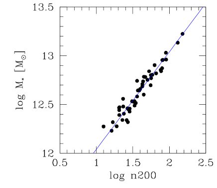
Figure 4: Richness vs stellar mass. There is tight relation between the number of bright red galaxies, $n200$, and the total stellar mass, $M_{\star}$, in clusters. The line marks a relation with slope one.

3.4 Results

Table 1 gives the found stellar masses within $r_{200}$ and their errors. Stellar mass errors are small in absolute terms, 0.08 dex on average, and also smaller than halo mass errors (i.e. errors from caustics, 0.14 dex on average).

Figure 4 plots the stellar mass, derived in the present paper, against the cluster richness $n_{200}$, i.e. the number of red galaxies brighter than $M_{V}=-20.0$ mag, derived for the very same sample by Andreon & Hurn (2010). There is a good agreement between the two quantities, which are basically two ways to summarise the luminosity content of clusters (by counting galaxies or photons):

$lgM_{\star}=(\log n200-2)+13.04\pm 0.03$

The slope of the regression is fixed to 1.0 (it is not a fit to the data) and the quoted error is just the formal error. For our sample, the two quantities, $lgM_{\star}$ and $\log n200$ are known with the same amount of precision (0.08 dex).

The good agreement between the two summaries of the cluster luminosity content is a confirmation of the correctness of the two derivations. We note, in fact, that the present derivation uses a more constrained model (a shape for the luminosity function and for background galaxy counts), and more (i.e. also fainter) data than the derivation of $n_{200}$ in Andreon & Hurn (2010). The proportionality of stellar mass and richness is in agreement with the very small, if any, dependency of the faint end slope of the luminosity function with richness (e.g. Garilli, Maccagni & Andreon 1999; Paolillo et al. 2001; Andreon 2004), and with the direct determination of Rines et al. (2004) from a small sample of 9 clusters. These authors consider, however, $lgM_{\star}$ and $\log n200$ integrated down the same limiting magnitude, differently from our choice.

3.5 Comparison with literature

Our stellar mass determination fundamentally differs from previous published works from three major points of view: a) in the way we choose the clusters to be studied; b) in the adopted reference radius; and c) in the performed analysis.

a) First and foremost, if a precise stellar mass within a reference radius of clusters have to be derived, it is strongly preferable (not to say essential) that:

i) the studied clusters are truly existing objects. Our clusters and groups are truly existing objects, with an extended X-ray emission and, on average, 208 spectroscopically confirmed members. Most of Giodini et al. (2009) systems are noisy X-ray detections which are ambiguous both in terms of detection and extent, “cleaned” by asking a spatial matching with an overdensity of galaxies to decrease contamination by point sources and blends of point sources misclassified as extended X-ray sources (Finoguenov et al. 2008). Only half of the ’surviving’ detections have three or more concordant redshifts (Giodini et al. 2009), and only a minority is currently spectroscopic confirmed, according to Gal et al. (2008), that show that three concordant redshifts occur frequently by chance in real redshift surveys (a further example is given in Sec 3.6 of Andreon et al. 2009 using the VVDS survey).

ii) the reference radius in which stellar masses have to be measured is known and individually measured. All our clusters have individually measured radii (by Rines and Diaferio 2006). Clusters in Gonzalez et al. (2007) and Giodini et al. (2009) have radii inferred from X-ray scaling relations assuming that these are scatter-free, contrary to observations (e.g. e.g. Stanek et al. 2006; Vikhlinin et al. 2009; Andreon & Hurn 2010). In other terms, these works assume that the radius appropriate for the studied clusters is the one of an average cluster having the same observable (e.g. X-ray flux), ignoring that clusters have a variety of radius values, even restricting the attention to those with a given value of the observable (say X-ray luminosity, it is just enough to think to cool-core and not cool-core clusters). In passing, the scaling adopted by Gonzalez et al. (2007) is said in agreement with Hansen et al. (2005), which is now known to return radii wrong by a factor two (Sheldon et al. 2007, Rykoff et al. 2008).

iii) the studied clusters are located in a narrow range of redshift, in order not to be obliged to assume an evolution on cluster scaling relation (e.g. how the $L_{X}$-mass scaling evolves) or on M/L. All our clusters are in the local universe ($z<0.1$), saving us from making an hypothesis on how to relate parameters (masses, virial radii, etc.) measured at widely different different redshifts. Other works (e.g. Giodini et al. 2009) consider objects in a large redshift range (e.g. $0.1<z<1$) and neglect the uncertainty on evolution.

b) We believe our adopted radius, $r_{200}$, a better choice for the determination of stellar masses than the radius adopted by other authors, $r_{500}$. First, $r_{500}$ is small enough that the stellar mass within $r_{500}$ depends on the precise definition of “center” (barycenter, BCG location, X-ray peak, etc). If the center is measured with a finite degree of accuracy (which is often the case), a small radius leads to a systematic underestimate of the stellar mass because of centroiding errors. If instead one pretends that the cluster center is coincident with the BCG location, then a systematic overestimate is introduced, because the observationally derived value will be boosted by the presence of the BCG. Systematics are strongly reduced if $r_{200}$ is used, as it encloses most of the cluster. The $r_{500}$ radius also makes an under-optimal use of the optical data, stellar masses have smaller error if $r_{200}$ is used in place of $r_{500}$, as it is fairly obvious ($r_{500}$ is only a few times the BCG size), and as we verified for our sample. Furthermore, the choice of a larger radius makes the BCG and intracluster light contribution small in percentage and thus their precise contributions largely irrelevant for the aim of determining the total amount of mass in stars (and in baryons). A larger than $r_{500}$ radius is also what is needed to compare with theory, because the latter has big difficulties in predicting the stellar mass fraction on such small scale. On the other end, the use of a radius larger than $r_{500}$ makes more complicate to compute the total baryon mass fraction, being the gas mass fraction usually measured at smaller radii.

c) For what concerns the analysis, the way we derived the integral of the luminosity function is rigorous: the use of the likelihood function for unbinned data is a significant improvement (Cash 1976; Sandage, Tammann & Yahil 1979; Andreon, Punzi & Grado 2005; Humphrey, Liu, & Buote 2009) above previous approaches that bin data, and even more above those that use simplified schemes, as quadrature sums, to combine errors (see Andreon, Punzi & Grado 2005 for details). Furthermore, differently from previous works, we do not identify the luminosity function, which is a positively defined quantity, with the difference of two galaxy counts, that may be negative. Our choice of marginalizing over the LF parameters is in agreement with axioms of probability and logic. Keeping some of them, e.g. $\alpha$ fixed, as in most literature papers, contradicts them. Finally, and differently from all other works, we allow each cluster to have its own faint end slope and characteristic magnitude, given that the luminosity function differs from cluster to cluster (e.g. Virgo and Coma clusters: Bingelli, Sandage, & Tammann 1988).

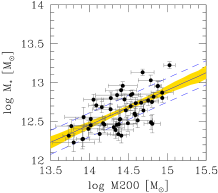
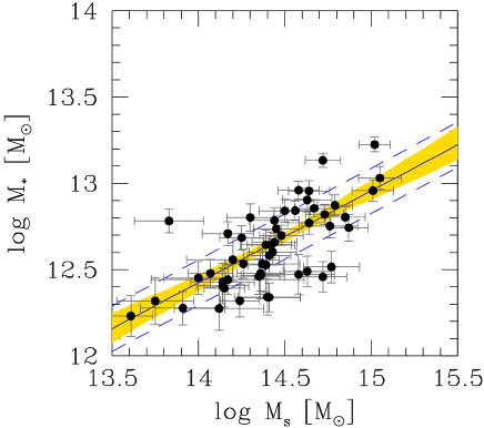
Figure 5: Stellar mass vs cluster mass scaling. The solid line marks The mean relation between stellar mass and halo mass is marked with a solid line, its 68 % uncertainty is shaded (in yellow). The dashed lines show the mean relation plus or minus the intrinsic scatter $\sigma_{scat}$. Error bars on the data points represent observed errors for both variables. The distances between the data and the regression line is due in part to the observational error on the data and in part to the intrinsic scatter. Left panel uses caustic masses, right panel uses velocity-dispersion based masses fixed by numerical simulations.

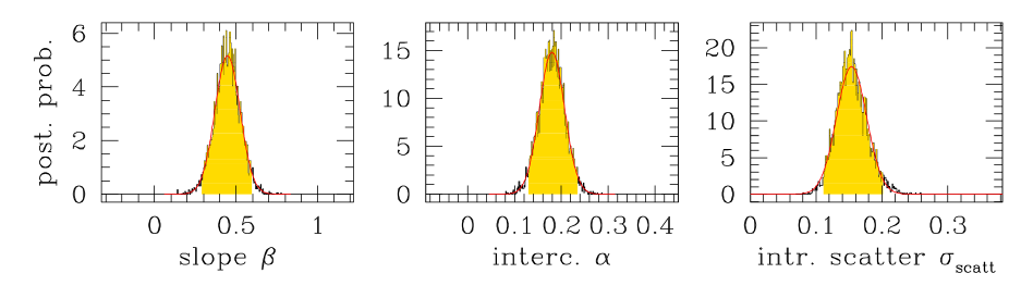
Figure 6: Posterior probability distribution for the parameters of the halo mass-stellar mass scaling. The black jagged histogram shows the posterior as computed by MCMC, marginalised over the other parameters. The red curve is a Gauss approximation of it. The shaded (yellow) range shows the 95 % highest posterior credible interval.

4 Collective analysis of the whole sample

4.1 Stellar mass vs halo mass

In order to fit the trend between stellar and total mass we use the statistical model (fit) detailed in the Appendix A. Essentially, our model assumes that the true stellar mass and true halo mass are linearly related with some intrinsic scatter but rather than having these true values we have noisy measurements of both stellar mass and halo mass, with noise amplitude different from point to point. In the statistics literature, such a model is know as an “errors-in-variables regression” (Dellaportas & Stephens, 1995) and has been widely used before, including more complex situations (e.g. Andreon 2006, 2008; Andreon et al. 2006, 2008a, 2008b, Andreon & Hurn 2010, Kelly 2007, etc.). The model is fully specified, and the code listed, in Appendix A.

Using the (fitting) model above, we found, for our sample of 52 clusters:

$$lgM_{\star}=(0.45\pm 0.08)\ (\log M200-14.5)+12.68\pm 0.03$$ (2)

(Unless otherwise stated, results of the statistical computations are quoted in the form $x\pm y$ where $x$ is the posterior mean and $y$ is the posterior standard deviation.)

The left panel of Figure 5 shows the relation between stellar mass and halo mass, observed data, the mean scaling (solid line) and its 68 % uncertainty (shaded yellow region) and the mean intrinsic scatter (dashed lines) around the mean relation. The $\pm 1$ intrinsic scatter band is not expected to contain 68 % of the data points, because of the presence of measurement errors.

Figure 6 shows the posterior marginals for the parameters: slope, intercept, and intrinsic scatter $\sigma_{scat}$. These marginals are well approximated by Gaussians.

The slope is very different from one, i.e. low mass clusters are not simple scaled-down version of high mass clusters: they have more stars per unit halo mass than their more massive cousins, in agreement with Girardi et al. (2000), and other works. Equivalently, the stellar mass fraction decreases with increasing stellar mass, as better shown in sec 4.3.

The intrinsic stellar mass scatter at a given halo mass, $\sigma_{scat}=\sigma_{lgM_{\star}|lgM200}$, is $0.15\pm 0.02$ dex. This is the intrinsic scatter, i.e. the term left after accounting for measurement errors. It is clearly non-zero (see right panel of Figure 6). This is a sort of “cosmic variance”: at a given halo mass, clusters are not all equal in terms of the amount of stars they have, but show a spread of stellar masses. Alternatively, the intrinsic scatter is a manifestation of an underestimate of the errors. This is unlikely to be the case, because an intrinsic scatter is seen also in gas masses and in numerical simulations of star and gas masses (later discussed), and therefore we need that errors on four different observables (observed gas and stellar masses, gas and stellar masses predicted in numerical simulations) are underestimated, which is unlikely. Next section addresses in detail a further hypothetical possibility, whether the intrinsic scatter of stellar masses is due to underestimated errors on caustic masses (underestimate that, even if present, does not explain anyway why a scatter is also seen in numerical simulations). No matter which is the source of the intrinsic scatter, its presence has a few consequences: first, larger cluster samples are requested to measure the average stellar mass fraction with a given precision. Second, and conversely, the existence of a non-zero intrinsic scatter is a technical complication to be accounted for in the determination of the trend between stellar mass (or stellar mass fraction) vs cluster mass. The intrinsic scatter is, as mentioned, rigorously accounted for in our fitting model.

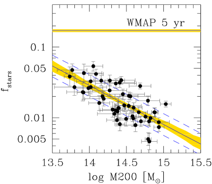
Figure 7: Stellar mass fraction. Symbols as in Figure 5. The fit is performed in the stellar vs total mass plane. The distances between the data and the regression line is due in part to the observational error on the data and in part to the intrinsic scatter. The WMAP 5 yr value and errors (Dunkley et al. 2009) are marked.

4.2 Checking caustic masses

Because of the relative novelty of caustic masses, and the hypothetical possibility that the intrinsic scatter on stellar masses might be due to an underestimate of caustic mass errors, we now replace caustic mass by a mass, $M_{s}$, derived from velocity dispersion using a relation calibrated with numerical simulations in Biviano et al. (2006). As shown in Andreon & Hurn (2010), the mass derived using the calibration in Evrard et al. (2008) gives almost indistinguishable numbers, because the two calibrations are almost identical for our clusters. Velocity dispersions are taken from Rines & Diaferio (2006).

To use the masses $M_{s}$ in place of the caustic ones, we need only write their values (and their errors) in the data file and run our fitting model, listed in Appendix. Mass errors are derived by combining in quadrature velocity dispersion errors (converted in mass) and the intrinsic noisiness of $M_{s}$ (12 %, from Biviano et al. 2006). We found:

$$lgM_{\star}=(0.53\pm 0.08)\ (\log M_{s}-14.5)+12.69\pm 0.03$$ (3)

with an intrinsic scatter of $0.13\pm 0.03$. By changing the source of halo masses, regression parameters (slope, intercept and intrinsic scatter) do not change. Therefore, the observed intrinsic scatter cannot be due to (unknown) systematics of caustic masses. Data and fit for velocity dispersion derived masses are shown in the right panel of Fig 5.

The insensitivity of our results to which mass is used is expected, because in Andreon & Hurn (2010) we show the absence of a gross offset or tilt between caustic and velocity-dispersion based masses, and that the error quoted for the caustic mass is as precise as (or as wrong as) the error quoted for the velocity dispersion-based mass.

To summarize, the scatter on the amount of stars that clusters contain at a given halo mass is not due to an un-accounted systematic of the halo mass.

4.3 Stellar mass fraction

Figure 7 plots the stellar mass fraction vs the cluster mass. The fraction is computed following its definition: it is the logarithmic difference of the stellar mass, $M_{\star}$, and the halo mass, $M200$. The fit has been performed in the stellar mass vs halo mass plane, and so derived errors are shaded in Figure 7. In addition to the exact analysis (marked with lines and shadings), we also report approximated errors, marked as error bars, based on just the error on stellar mass, for simplicity. Our fit to the data accounts for the intrinsic scatter, and also simply solves a further problem that affects previous analysis: the fit in the fraction vs halo mass plane performed by other authors (e.g. Gonzalez et al. 2007; Giodini et al. 2009) has the halo mass both on the abscissa and in the ordinate (it is at the denominator of the fraction). As a consequence, the values fitted by other works have correlated errors. However, past works used fitting methods that assume errors to be uncorrelated. Our solution, fitting in the stellar mass vs halo mass, where measurement errors are uncorrelated, solves this problem too.

The decrease in the stellar mass fraction is stunning, with a slope equals to $-1+0.45\pm 0.08=-0.55\pm 0.08$. The quality of this result can be better appreciated after noting that the trend above was considered not constrained by data in recent papers: Allen et al. (2008) assume a stellar mass fraction proportional to the gas fraction (when instead the two fractions have opposite dependencies with halo mass, as shown in Figure 8 and discussed in Sec 4.4), whereas Ettori et al. (2009) considered a number of recipes, because of lack of conclusive data. Bode et al. (2009) consider the slope as a free (i.e. not constrained by any stellar fraction observation) parameter.

The value of the slope is robust to systematic errors affecting the conversion factor from luminosity to stellar mass. In fact, to bias the found slope, we need that the $M_{\star}/L$ value of the galaxies depends on the mass of the cluster. It is difficult to imagine why the initial stellar mass function (which largely regulate $M_{\star}/L$ value) should be different in galaxies that are in clusters of different masses. Furthermore, the $M/L$ values in Capellari et al. (2006) comes from galaxies lying in halos of different masses. Finally, the fundamental plane shown no halo-mass or environmental dependency (Pahre et al. 1998).

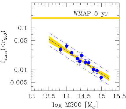
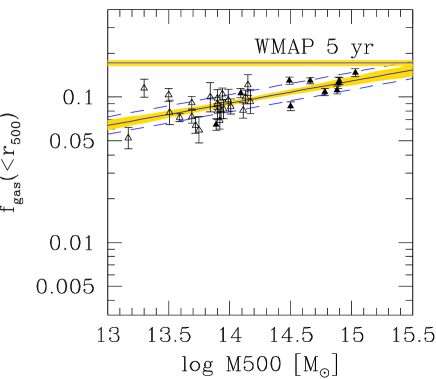
Figure 8: Stellar and gas mass fraction. Left panel: Closed (large, blue) circles mark the stellar mass fraction in stacks of 5 clusters each, with the exception of the most massive point, composed by just two clusters. Error bars mark approximate errors. The solid line and shaded region marks the mean model and its (rigorous) 68 % confidence error, fitted on individual data points in the stellar vs total mass plane. Right panel: Open/solid triangles mark the gas mass fraction from Sun et al. (2009) and Vikhlinin et al. (2006), respectively. The solid line and shaded region mark the mean model and its (rigorous) 68 % confidence error, derived by us using their data. The WMAP 5 yr value and errors (Dunkley et al. 2009) are marked in both panel.

The left panel of Figure 8 shows the fraction of mass in stars, but after stacking clusters in bin of five clusters each, with the exception of the highest mass bin, composed by two clusters only. The figure reports both the rigorous computation of errors (shading), computed in the stellar vs total mass plane, and approximated errors (error bars). For the latter, we only consider the largest source of error, the intrinsic scatter, and we neglect other sources of errors, as the uncertainty of the intrinsic scatter or the observational error, accounted for in our rigorous computation (which also account for the covariance of all sources of errors).

After binning, the decrease in the stellar mass fraction becomes clearer, due to the smaller error bars of our cluster stacks.

The horizontal lines in Figure 7 and 8 mark the Universe baryon fraction from the five-year WMAP results in Dunkley et al. (2009). 68 % credible intervals are shaded. This has to be taken as an upper limit to the stellar mass fraction, because there are other baryons in clusters. Stars account for only about one third at most of all baryons.

Table 2 lists derived stellar mass fractions and their errors.

Table 2: Stellar and gas fractions.

$\log M$	$\log f_{stars}$	$\log f_{gas}$
	$(<r_{200})$	$(<r_{500})$
13.1		$-1.18^{0.03}_{-0.03}$
13.3		$-1.15^{0.02}_{-0.03}$
13.5		$-1.12^{0.02}_{-0.02}$
13.7	$-1.38^{0.06}_{-0.06}$	$-1.09^{0.02}_{-0.02}$
13.9	$-1.49^{0.05}_{-0.05}$	$-1.06^{0.01}_{-0.02}$
14.1	$-1.60^{0.04}_{-0.04}$	$-1.03^{0.01}_{-0.01}$
14.3	$-1.71^{0.03}_{-0.03}$	$-1.00^{0.01}_{-0.01}$
14.5	$-1.82^{0.03}_{-0.03}$	$-0.97^{0.02}_{-0.02}$
14.7	$-1.93^{0.03}_{-0.03}$	$-0.94^{0.02}_{-0.02}$
14.9	$-2.04^{0.04}_{-0.04}$	$-0.91^{0.03}_{-0.02}$
15.1		$-0.87^{0.03}_{-0.03}$

The mass indicated in column 1 is measured within the aperture specified in the fraction definition.

4.4 Gas mass fractions

Vikhlinin et al. (2006) and Sun et al. (2009) data on the fraction of matter in the hot intergalactic gas are plotted in the right panel of Figure 8, after converting them for minor differences in the adopted cosmological parameters.

Masses and gas mass fractions are measured within $r_{500}$. Because of asymmetrical errors on $f_{gas}$ we assume Gaussian errors on $\log f_{gas}$ so that our previous fitting model can be applied without any change (apart for reading “gas fraction” where “stellar mass” is written). We found:

$$\log f_{gas}=(0.15\pm 0.03)\ (\log M500-14.5)-0.97\pm 0.02$$ (4)

with an intrinsic scatter of $0.06\pm 0.01$ dex. The right panel of Figure 8 shows the derived mean $f_{gas}$ vs halo mass fit (slanted solid line) and its 68 % uncertainty (shaded yellow region) and the mean intrinsic scatter (dashed lines) around the mean relation.

Intercept and slope posteriors are Gaussian shaped, whereas the intrinsic scatter posterior is a bit skewed, as a Gamma function (figure not shown). Our mean relation is similar to Sun et al.’ (2009) best fit. Their work, however, uses a similar, but not identical, cluster sample and a different fitting model. Our intrinsic scatter value cannot be compared with their, because these authors, although note a scatter, do not report its value, if measured at all.

Similarly to stellar masses and stellar mass fractions, gas fractions display an intrinsic variance, i.e. intrinsic differences from cluster to cluster. The scatter is not bounded to low mass systems, but is apparent to all masses (see Figure 8, and Vikhlinin et al.’ 2006 fig. 21), differently from some past claims of a spread at group (low) mass only. We emphasise that Vikhlinin et al. (2006) and Sun et al. (2009) selected and studied a sample of clusters and groups that, from X-ray images, appeared relaxed. Therefore, the found spread of gas fractions at a given cluster mass is not due to the presence in the sample of clusters manifestly out of equilibrium (e.g. merging).

Table 2 lists derived gas mass fractions and their errors.

Given the importance of our claim that intrinsic scatter is not restricted to low mass systems only, let’s look for an independent, although not equally precise, measurement.

The existence of an intrinsic scatter at high masses is confirmed by our analysis of gas fractions in Ettori et al. (2009). We took their $f_{gas}$ values and errors, quoted at 68.3 % level of confidence, from their Table 1. Their quoted errors are symmetric, and Gaussian distributed, because Eq. 7 in Ettori et al. (2009) only holds in this case. A Gaussian likelihood for $f_{gas}$ is mathematically impossible, because a Gaussian is strictly positive everywhere on all the real axis, including impossible values for a fraction, those outside the $[0,1]$ range. It is therefore unsurprising that several of their quoted 68.3 % confidence intervals include unphysical (negative) values for a fraction. In order to select, among their measurements, those for which the Gaussian approximation is an acceptable approximation, we select from their sample only the best measurements, defined those having a $f_{gas}$ determination with a S/N ($=f_{gas}/err$) larger than 3. This operation removes 31 out 52 of their clusters. We then fit the gas fraction vs the cluster temperature (the mass proxy listed in their paper) of the remaining 21 clusters, accounting for errors on both variables and a possible intrinsic scatter. As in previous fitting, we re-use the fitting model given in Appendix A, we only need to read $f_{gas}$ and $kT$ where log stellar mass and log halo mass is written. We found:

$$f_{gas}=(0.000\pm 0.004)\ (kT-8)+0.14\pm 0.01$$ (5)

with an intrinsic scatter of $0.03\pm 0.01$ on $f_{gas}$. Fig 9 shows the derived mean $f_{gas}$ vs cluster temperature fit (solid line) and its 68 % uncertainty (shaded yellow region) and the mean intrinsic scatter (dashed lines) around the mean relation. All clusters have $kT>5$ keV, i.e. are very massive. Yet the intrinsic scatter is not zero, confirming that the intrinsic scatter in the gas mass fraction is not reserved to low mass clusters only. The large majority (17 out 21) of the fitted clusters have an observational error smaller than the intrinsic scatter. Therefore, by far the largest source of uncertainty in the determination of the average gas mass fraction of clusters (and of the baryon fraction of the universe, derived from these measurements) is the intrinsic scatter, and not the measurement error.

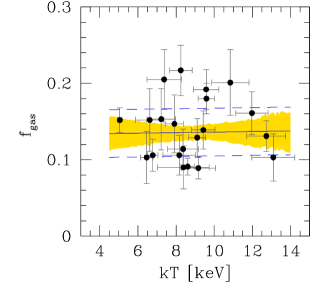
Figure 9: The gas mass fractions. Symbols are as in Fig 5. Error bars on the data points (from Ettori et al. 2009) represent observed errors for both variables. The distances between the data and the regression line is due in part to the observational error on the data and in part to the intrinsic scatter.

The value of the intrinsic scatter determined for the Ettori et al. (2009) sub-sample cannot be easily compared with the one derived for Vikhlinin et al. (2006) and Sun et al. (2009) for three reasons at least: first, the intrinsic scatter is the part of the scatter not due to observational errors. Therefore, its amplitude relies on the assumption that observational errors are precisely measured. As mentioned, Ettori et al. (2009) quoted errors are noisy estimate of the true errors (see Andreon & Hurn 2010 about how to deal with noisy errors). Second, the scatter derived for the Ettori et al. (2009) sample is measured on a linear gas fraction scale, whereas the one for the Vikhlinin et al. (2006) and Sun et al. (2009) is on a logarithmic scale (compare the left hand side of Eq.s 4 and 5), and a Gaussian scatter on one scale does not translate on a Gaussian scatter on the other scale. Finally, the scatter measured with the Ettori et al. (2009) data is at a given temperature, not at a given mass, as the one measured with Vikhlinin et al. (2006) and Sun et al. (2009) data. If the above caveats are ignored, then one find a good qualitative agreement between the two determinations of the intrinsic scatter after an approximate conversion to a common scale.

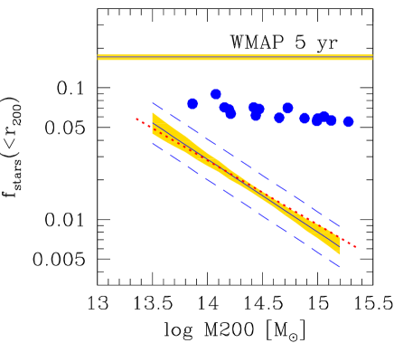
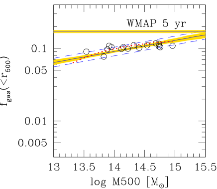
Figure 10: Comparison between observed and theoretical stellar (left panel) and gas (right panel) fractions. Solid lines and shaded regions mark our observational constraints on the stellar and gas mass fractions. Open and closed points mark theoretical gas and stellar mass fractions, respectively, observed in gasdynamical simulation with cooling and star formation of Kravtsov et al. (2005) and Nagai et al. (2007). The dotted red lines are the predictions of the model by Bode et al. (2009).

The existence of an intrinsic scatter in $f_{gas}$ (both at a given mass and at a given Temperature) must surprise all those who believe that, having clusters collected material from a large region, their content should be representative of the mean matter content of the universe (White et al. 1993). The measured intrinsic scatter implies that when taken individually the regions in which clusters and groups collected matter, a few tens of Mpc, are yet not representative, in terms of gas content and therefore in the baryon content (at large masses $f_{gas}$ is the largest baryon contributor) of the mean matter content of the Universe, i.e. each region has a gas, and thus baryon, content that differs from the average by more than the observational error. The existence of an intrinsic scatter on $f_{gas}$ does not preclude the use of the gas or baryon mass fraction as determined in clusters for cosmological tests, it only decrease its efficiency (a larger sample is required to achieve the same precision), and oblige us to address selection effects, i.e. to inquire if studied clusters are representative, in terms of $f_{gas}$, to the population present in the Universe, or are a biased subsample. Therefore, cosmological constraints derived from $f_{gas}$ ignoring intrinsic scatter and $f_{gas}$ selection function (e.g. Ettori et al. 2009) are optimistically estimated, and, perhaps, biased.

4.5 Stellar and gas mass fractions

The comparison of right and left panel of Figure 8 shows that the halo mass at which stars and gas contribute equally to the total halo baryonic content is near $10^{13.5}$ solar masses (roughly, $M200\approx 1.5\ M500$).

Figure 10 compare our observational constraints and theoretical predictions on the stellar (left panel) and gas (right panel) mass fraction. We consider gasdynamic simulations of Kravtsov et al. (2005) and Nagai et al. (2007). These simulations are performed in a (simulated) universe with a slightly too low (compared to WMAP5) baryon fraction ($0.14$ vs $0.17$). Therefore we revise upward fractions derived in simulations by $0.17/0.14$. Stellar mass fractions (Kravtsov 2009, priv. comm.) are measured at $r_{200}$ in the simulations, as for data. Gas mass fraction for the very same simulations are taken from Nagai, Vikhlinin & Kravtsov (2007), and are measured within $r_{500}$, as for data. Gas fractions have been revised upward by $0.17/0.14$, for the same reason as stellar fractions. The predicted fraction of matter in gas (open points, right panel) is near to the observed gas mass fraction, as commented in Kravtsov et al. (2009) and Nagai et al. (2007). Note in particular that simulated clusters also displays a spread of gas and stellar mass fractions at a given halo mass, as real clusters.

As remarked by Kravtsov et al. (2009) and Gonzalez et al. (2007), the predicted stellar mass fraction (close points, left panel) is off from the observed one (slanted solid line), and more evidently so in our paper than in previous works, given our more precise observational determination. Both the slope and the intercept of the simulations are in flagrant disagreement with the observed values. Gasdynamic simulations with star formation of Fabjan et al. (2009) show a very similar behaviour to Kravtsov et al. (2009) and Nagai et al. (2007) simulations: the temperature-mass scaling and the gas mass fraction can only be reproduced if star formation is allowed, but in such case the predicted stellar mass fraction (similar in the two sets of simulations) is off.

The mismatch between predicted and observed stellar mass fractions is not of secondary importance in the cluster model because of the strict interplay of the stellar and gas components. First, if less stars need to be formed, then more gas is left, and thus the current agreement between predicted and observed gas mass fractions is corrupted. Second, the gas component responds to the feedback of the stellar component (e.g. Nagai et al 2007; Fabjan et al. 2009). If the stellar part of the model have to be altered, changes on the gas predictions (e.g. X-ray scaling relations) occur. Unfortunately, the agreement of gas-related quantities, as the temperature-mass scaling, holds in current models for wrong stellar content predictions. Therefore, observations on the stellar mass fraction presented in this paper give a challenging constraint to theories of cluster formation.

Bode et al. (2009) presented a semi-analytical cluster model, i.e. they inserted a number of recipes on an N-body simulation. They concluded that if the stellar mass fraction has a logarithmic slope of $-0.49$, then there is no need of a supplementary feedback, i.e. in addition to the stellar one, to match the gas mass fraction and X-ray scale relations (temperature-mass, $Y_{x}$-mass). Our observed stellar mass fraction has a logarithmic slope of $-0.55\pm 0.08$ is consistent with the slope required to avoid supplementary feedback in the Bode et al (2009) model.

In the Bode et al. (2009) model, this is a real model prediction, it has not adjusted to match previous observational data on the stellar mass fraction slope. At the contrary, the remaining model parameters commented below have been adjusted to fit observations, reducing the significance of the agreement between “predicted” and observed values. The intercept of the model stellar mass fraction vs mass, kept fixed by Bode et al. (2009) to the Lin et al. (2003) value, also agrees with our observational determination: the Bode et al. (2009) model stellar mass fraction (dotted red line, left panel) is fully enclosed in the 68 % confidence band of our observational determination, i.e. it is in remarkable agreement. Similarly, the Bode et al. (2009) model gas mass fraction (dotted red line, right panel) is in reasonable agreement with our summary of observational data. If the simple Bode et al. (2009) cluster model is not an over-simplified description of true existing clusters, then the slope of the stellar mass fraction vs halo mass we determine in this paper implies that AGN feedback is not needed, at least to reproduce X-ray scaling relations and stellar and gas mass fractions.

A couple of technical points are worth mention: in the Bode et al. (2009) model, the stellar mass fraction is determined within the virial radius, as our observational determination is, but is parametrised as a function of $M(<r_{500})$, that we converted to $M200=M(<r_{200})$, assuming a NFW profile and a concentration of 3. Instead, gas mass fractions are computed within $r_{500}$ both for the model and for the data.

4.6 Stellar + gas mass fraction

In order to add the stellar and gas mass fractions to get the total fraction of baryons we need to address some issues.

First, stellar and gas mass fractions are measured inside different reference radii ($r_{200}$ and $r_{500}$). Simulations shows that the region inside $r_{500}$ is depleted, if any, by a small and poorly determined amount of the order of 2 to 10 % (Ettori et al. 2006, Kravtov et al. 2005). We adopt a 5 % correction with a $3\sigma$ error of 6 %.

Second, we need to convert the fit in Eq. 3 from a fit vs $M500$ to a fit vs $M200$. The mass conversion is performed assuming a NFW of concentration 3. Any scatter of the concentration at a given mass or any change of the mean concentration with mass has little effect on this conversion, because Eq. 3 is the mean relation, and it is linear and shallow.

Third, the gas and stellar masses measurements are assumed to be independent (which is true), and the intrinsic scatter of gas and stellar mass fractions around the mean are assumed to be unrelated each other (which is unknown given the available data).

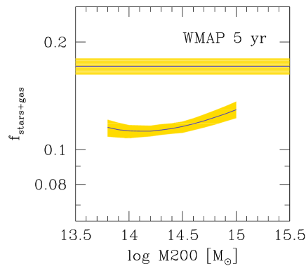
Figure 11: Baryon fraction. The solid curve and shaded region mark the mean the observationally measured $f_{stars}+f_{gas}$ and its (rigorous) 68 % confidence error. The WMAP 5 yr baryon fraction value and error (Dunkley et al. 2009) are also marked.

Figure 11 displays the total fraction in baryons, $f_{stars+gas}$, as a function of cluster mass, in the range where both $f_{stars}$ and $f_{gas}$ are both constrained by the data, $13.7\leq\log M200\leq 15.0$ solar masses. These values and errors come from the fit on individual data points in the stellar vs total mass plane and in gas mass fraction vs total mass, with the mentioned (minor) corrections. The variety of cluster properties at a given mass is fully accounted for by our derivation of $f_{stars+gas}$.

Two points are striking in Figure 11: a) we observe an almost constant baryon fraction in the studied mass range, the increase of the gas mass fraction being approximatively compensated by the decrease of the stellar mass fraction; and b) WMAP-derived baryon fraction differs from our estimate by about $6$ sigma’s.

Readers interested in inferring the values of cosmological parameters from our measured baryon fraction should remember that our own determination of the baryon fraction has been derived for an assumed set of cosmological parameters (listed at the end of the introduction), instead of being marginalised over the uncertainty of cosmological parameters. The latter operation matters for estimates of cosmological parameters, which is, however, beyond the scope of the present paper.

How can one reconcile the observed value of the baryon fraction in clusters with the larger value derived from WMAP?

We explore few possibilities in turn.

First, might a large bias on $f_{stars}$ be present? It is hard to be accommodated, because in order to boost the stellar mass fraction one need:

a) that $L_{tot}$ is largely underestimated. This is only possible below the observed range of galaxy luminosities (we reach $-19.3<M_{r}<-15.7$ mag, depending on redshift) and requires that the luminosity function keeps a diverging slope (i.e. $\alpha\la-2$) for a large magnitude range below the one considered in this work. However, clusters with very deep observations do not display such a feature, down to $M_{V}\sim-11$ (e.g. Sandage, Binggeli, & Tammann 1985; Andreon & Cuillandre 2002; Andreon et al. 2006; Boué et al. 2008, etc); or

b) that the observed (and adopted) $M/L$ conversion is biased;

c) that the intracluster light (that we emphasise not to include the light from galaxy outer halos, from the BCG and from undetected galaxies, see Sec 3.2) is about 5 mag arcsec^-2 brighter that the value measured in Zibetti et al. (2005). This number has been derived basically reverting the performed operations to derive stellar masses: we first compute the missing baryon fraction (WMAP $f_{baryon}$ value minus $f_{star+gas}$), we multiply it by the cluster mass within $r_{200}$ to derive missing stellar masses. We then convert the latter in luminosities with the assumed $M/L$ value, and project them in the plane of sky (i.e. converting back from values within spheres to within cylinders). Finally, mean brightness is derived from the luminosity value, accounting for the cluster size (i.e. adding $2.5\log\pi r^{2}_{200}$, with radii in arcsec). The missing mass implies a mean (within $r_{200}$ and averaged over the sample of 52 clusters) surface brightness of $\mu_{r}\sim 26.5$ mag arcsec^-2. The latter value is, as mentioned, fairly too bright to match the observational value.

Even if a large bias on $f_{stars}$ is there (which is implausible) for a still un-identified reason, this leaves untouched the disagreement with the WMAP-derived value at high cluster masses, where the stellar contribution is minor.

Second, $f_{gas}$ estimates might be systematically low. Systematic biases, in addition to depletion already accounted for, of the gas mass fraction are discussed in Ettori et al. (2009), Allen et al. (2008) and reference therein. Our reading of these papers is that the gas mass fraction is free from important unknown systematics, otherwise these authors would not attempt to constraint cosmological parameters using it. Therefore, we are tempted to exclude systematics on $f_{gas}$, although, of course, direct measurements of $f_{gas}$ within $r_{200}$ would be preferable. We only known a single $f_{gas}$ measurement at $r_{200}$, by George et al. (2009). They found a fraction $0.02\pm 0.02$ higher at $r_{200}$ than at $r_{500}$, in agreement with our assumed correction.

Third, we might miss some other sources of baryons. Fukugita, Hogan & Peebles (1998) explored this issue, and concluded that stars and the hot intergalactic gas contain the large majority of baryons.

Therefore, we are obliged to consider the possibility that the WMAP baryon fraction is wrong in some sense. The value derived by WMAP is the value of the baryon content assuming that it is universal, i.e. equal to an unique value everywhere without any scatter or dependency with anything (say halo mass). This paper clearly shown that $f_{stars}$ and $f_{gas}$ are both not-universal: these fractions have a mass dependency. Furthermore, there is also a spread of both the stellar and gas mass fraction at a given mass. In absence of a fine tuning between the two fractions (a stellar mass excess being compensated by a gas deficit, which is hard to obtain given their widely different contributions at the two ends of the halo mass function), $f_{baryons}=f_{stars}+f_{gas}$ should display an intrinsic scatter. The hypothesis of a possible not universal baryon fraction, although surprising, is not totally new and has been already proposed by Holder, Nollett, & van Engelen (2009). It would be interesting to known what would be the CMB-derived constraint on the baryon fraction if it was allowed to display a variance.

It is also possible that the baryon fraction is larger than the WMAP value at locations that we have not sampled, halos with masses lower than $10^{13.5}$ solar masses and outskirts of clusters. For the latter, there is some evidence (e.g. Rines et al. 2004). A larger-than-WMAP baryon fraction at these locations might compensate the lower-than-WMAP value in the studied (portion of) clusters and groups. This possibility assumes a non-universality of the baryon fraction. In such case, WMAP-derived baryon fraction might require a new derivation, under this less restrictive hypothesis.

Finally, McCarthy et al. (2007) suggested that the problem may sit in an underestimate of the denominator of the WMAP baryon fraction, i.e. in $\Omega_{m}$.

Although we have no solved the baryon discrepancy, we can exclude almost for sure that the stellar fraction is responsible for the difference between cluster and global baryon fraction and we identify possible points that require investigation.

4.7 Comparison with previous works

Our results are in qualitatively agreement with previous results (Gonzalez et al. 2007; Giodini et al. 2009), displaying an offset between the measured total baryon fraction and the WMAP value, and a decreasing stellar mass fraction with increasing mass. Some specific results might instead differ from some published results, for example, we do not confirm the Giodini et al. (2009) claim that the baryonic fraction increases with mass. However, our statements are fundamentally different from those published in other works.

We have already discussed, in sec 3.5, about the advantages of an accurate analysis of the data, of studying a sample of truly existing clusters located in a narrow range of redshift and having individually measured, and large, reference radii. We continue along the same line by noting that the cluster mass enters in the stellar mass fraction (it is at the denominator of the fraction), and thus is certainly an advantage to study clusters with known and precisely measured masses, instead of those with noisy or unknown masses. Our sample has accurate cluster masses derived under parsimonious hypothesis, that does not require the cluster being in dynamical or hydrostatic equilibrium, from the caustic analysis of Rines & Diaferio (2006) of about 208 galaxy members per cluster, on average. Instead, Gonzalez et al. (2007) masses are derived from velocity dispersion computed on small samples and with Beers et al (1990) estimators. These velocity dispersions (and masses) have low reliability (Andreon et al. 2008; Andreon 2009; Gal et al. 2008). Giodini et al. (2009) assume that mass is proportional to a poorly estimated X-ray luminosity without any scatter, when instead the two quantities display a large scatter (e.g. Stanek et al. 2006; Vikhinin et al. 2009; Andreon & Hurn 2010), it is just enough to remember the existence of cool-core clusters.

A second key difference between our and other works lays in performing an analysis that do not contradict the expected and observed spread in cluster properties at a given mass. Galaxy groups and clusters are the result of the assembly history of dark matter halos, and also shaped by star formation processes affecting the gas. These physical processes (and possibly other) lead to multivariate outcomes and produce an intrinsic spread in the distribution of the observed properties of groups and clusters, a spread that is readily apparent in any stellar or gas mass fraction vs cluster mass plot, such as our Figure 7 or 8. The spread manifest itself also as a variance of concentrations (and thus $r_{200}$) at a given cluster mass. Therefore, it is of paramount importance to account for the variance of cluster properties at a given cluster mass. Previous analysis fail to account for the above, having all assumed instead that clusters are identically equal at a fixed mass (or mass proxy). For example, Giodini et al. (2009) assume that all clusters of a given X-ray luminosity have the same size. Our analysis allows a variance in the cluster properties at a given halo mass. Finally, we have already noted that our analysis avoid the use of fitting methods in conditions where they must not be used.

In spite of our accounting of a larger number of error terms, we are able to reject the WMAP value at “much more sigma’s” than previous works, $6$ vs $3.2$ (Gonzalez et al. 2007) or $\sim 5$ (Giodini et al. 2009). This is the result of a different choice of the data and cluster sample: we choose clusters with accurate masses, good photometry and low galaxy background contribution, i.e. nearby clusters with caustic masses.

5 Summary

We analysed a sample of 52 clusters with precise and hypothesis-parsimonious measurements of mass, derived from caustics based on about 208 member velocities per cluster on average, and with measured $r_{200}$ values. We found that low mass clusters and groups are not simple scaled-down version of their massive cousins in terms of stellar content: lighter clusters have more stars per unit cluster mass. The same analysis also shows that the stellar content of clusters displays an intrinsic spread at a given cluster mass, i.e. clusters are not similar each other in the amount of stars they contain, not even at a fixed cluster mass. The amplitude of the spread in stellar mass, at a fixed cluster mass, is $0.15\pm 0.02$ dex. The stellar mass fraction depends on halo mass with (logarithmic) slope $-0.55\pm 0.08$. These results are confirmed by adopting masses derived from velocity dispersion.

The intrinsic scatter at a fixed cluster mass we determine for gas mass fractions taken from literature, is smaller, $0.06\pm 0.01$ dex. The intrinsic spread is not restricted to low mass systems only, but extend to massive systems. Since the studied systems look relaxed in X-ray images, the found spread is not due the presence in the sample of clusters manifestly out of equilibrium (e.g. merging). The non-zero intrinsic scatter of the gas mass fraction decreases the efficiency of $f_{gas}$ for cosmological studies, and asks to inquire about whether studied samples are representative, in terms of $f_{gas}$, to the population of clusters in the Universe.

The intrinsic scatter in both the stellar and gas mass fraction is a distinctive signature that when taken individually the regions in which clusters and groups collected matter are yet not representative, in terms of stellar and gas content and therefore in the baryon content, of the mean matter content of the Universe.

The observed stellar mass fraction values are in marked disagreement with gasdynamics simulation with cooling and star formation of clusters and groups. Instead, amplitude and cluster mass dependency of observed stellar mass fraction are those requested not to need any AGN feedback to describe X-ray scale relations and gas and stellar mass fractions in simple semi-analytic cluster models.

By adding the stellar and gas masses, or, more precisely speaking, by fitting both them and accounting for the intrinsic variance of both quantities, we found that the baryon fraction is fairly constant for clusters and groups with $13.7<\log M200<15.0$ solar masses and it is offset from the WMAP-derived value by about $6$ sigmas. The offset is unlikely to be due to an underestimate of the stellar mass fraction and could be related to the possible non-universality of the baryon fraction, pointed out by our measurements of the intrinsic scatter.

Our analysis is the first that does not assume that clusters are identically equal at a given halo mass and it is also more accurate in many aspects than previous works. The data and code used for the stochastic computation are distributed with the paper.

Appendix A Model listing and coding

In this section we give the listing of the full model, and its coding in JAGS.

Observed values of halo and stellar mass ($obslgM200$ and $obslgM_{\star}$, respectively) have a Gaussian likelihood.

$$obslgM200_{i} \sim \mathcal{N}(lgM200_{i},errlgM200^{2}_{i})$$ (6)

$$obslgM_{\star,i} \sim \mathcal{N}(lgM_{\star,i},errlgM_{\star,i}^{2})$$ (7)

The tilde symbol reads “is drawn from”, and the symbol $\mathcal{N}(y,\sigma^{2})$ denotes a Gaussian centered on $y$ with variance $\sigma^{2}$.

True values of stellar and halo mass are linearly related (on a log scale), with an intrinsic scatter $\sigma_{scat}$.

$$z_{i} = \alpha+12.5+\beta\ (lgM200_{i}-14.5)$$ (8)

$$lgM_{\star,_{i}} \sim \mathcal{N}(z_{i},\sigma^{2}_{scatt})$$ (9)

Masses are re-centred, purely for computational advantages in the MCMC algorithm used to fit the model (it speeds up convergence, improves chain mixing, etc.). Please note that the relation is between true values, not between observed values, which may be biased.

Uniform priors are taken: the halo mass, $obslgM200$, has a strictly uniform prior; the intercept, $\alpha$ has a zero mean Gaussian with very large variance; the slope, $\beta$, has a uniform prior on the angle (that becomes a Student $t$ distribution for the angular coefficient), because we do not want that cluster properties depends on astronomer rules to measure angles (see Andreon 2006, and Andreon & Hurn 2010 for a discussion); $1/\sigma^{2}_{scat}$ has a Gamma distribution with small values for its parameters, as in Andreon & Hurn (2010). This has the welcome property that the intrinsic scatter variable is positively defined, as the intrinsic scatter is. In symbols:

$$lgM200_{i} \sim \mathcal{U}(0,500)$$ (10)

$$\alpha \sim \mathcal{N}(0.0,10^{4})$$ (11)

$$\beta \sim t_{1}$$ (12)

$$1/\sigma^{2}_{scatt} \sim \Gamma(10^{-5},10^{-5})$$ (13)

Our model makes weaker assumptions than other models adopted in previous analysis, and plainly states what is actually also assumed by other models (e.g. the conditional independence and the Gaussian nature of the likelihood), also removing approximations adopted in other approaches.

For the stochastic computation and for building the statistical model we use Just Another Gibb Sampler (JAGS, Plummer 2008). JAGS, following BUGS (Spiegelhalter et al. 1995), uses precisions, $\tau=1/\sigma^{2}$, in place of variances $\sigma^{2}$. The arrow symbol reads “take the value of”. Normal, t, and Gauss distributions are indicated with dpois, dt, dgamma, respectively.

model
{
for (i in 1:length(obslgMstar)) {
  obslgM200[i] ~ dnorm(lgM200[i],tau.lgM200[i])
  lgM200[i] ~ dunif(0,500)

  obslgMstar[i] ~ dnorm(lgMstar[i],tau.lgMstar[i])
  z[i] <- alpha+12.5+beta*(lgM200[i]-14.5)
  lgMstar[i] ~ dnorm(z[i], prec.intrscat)
  }
intrscat <- 1/sqrt(prec.intrscat)
prec.intrscat ~ dgamma(1.0E-5,1.0E-5)
alpha ~ dnorm(0.0,1.0E-4)
beta ~ dt(0,1,1)
}

The code above, which is an almost literal translation of equations A1 to A8, is only about 10 lines long in total, about two orders of magnitude shorter than any previous implementation of a regression model (e.g. Kelly 2007, Andreon 2006, Akritas & Bershady 1996). The model is quite general, and applies to every quantities linearly related, with Gaussian errors, and with an intrinsic scatter. For example, in this paper the same model (and program) has been used for the $f_{gas}$ vs mass, and $f_{gas}$ vs temperature scaling. The same fitting model can be used for, say, the $L_{x}-\sigma_{v}$, richness–mass and halo occupation number vs mass scalings.

References

- Adelman-McCarthy & for the SDSS Collaboration (2007) Adelman-McCarthy, J. K., et al. (SDSS Collaboration), 2008, ApJS 175, 297
- Akritas & Bershady (1996) Akritas M. G., Bershady M. A., 1996, ApJ, 470, 706
- Allen et al. (2008) Allen S. W., Rapetti D. A., Schmidt R. W., Ebeling H., Morris R. G., Fabian A. C., 2008, MNRAS, 383, 879
- Andreon (2002) Andreon, S. 2002, A&A, 382, 495
- Andreon (2004) Andreon S., 2004, A&A, 416, 865
- Andreon (2006) Andreon, S. 2006, MNRAS, 369, 969
- Andreon (2008) Andreon S., 2008, MNRAS, 386, 1045
- (8) Andreon, S. 2009, in Bayesian Methods in Cosmology, Cambridge University press222 ttp://www.cambridge.org/uk/catalogue/catalogue.asp?isbn=9780521887946
- Andreon & Cuillandre (2002) Andreon S., Cuillandre J.-C., 2002, ApJ, 569, 144
- (10) Andreon, S. & Hurn, M., 2010, MNRAS, in press (arXiv:1001.4639)
- Andreon et al. (2006) Andreon, S., Cuillandre, J.-C., Puddu, E., & Mellier, Y. 2006, MNRAS, 372, 60
- Andreon et al. (2008) Andreon, S., De Propris, R., Puddu, E., Giordano, L., & Quintana, H. 2008a, MNRAS, 383, 102
- Andreon et al. (2008) Andreon, S., Puddu, E., de Propris, R., & Cuillandre, J.-C. 2008b, MNRAS, 385, 979
- Andreon et al. (2005) Andreon, S., Punzi, G., & Grado, A. 2005, MNRAS, 360, 727
- Binggeli et al. (1988) Binggeli, B., Sandage, A., & Tammann, G. A. 1988, ARAA, 26, 509
- Biviano & Girardi (2003) Biviano A., Girardi M., 2003, ApJ, 585, 205
- Blanton et al. (2001) Blanton, M. R., et al. 2001, AJ, 121, 2358
- Bode, Ostriker, & Vikhlinin (2009) Bode P., Ostriker J. P., Vikhlinin A., 2009, ApJ, 700, 989
- Boué et al. (2008) Boué G., Adami C., Durret F., Mamon G. A., Cayatte V., 2008, A&A, 479, 335
- Bruzual & Charlot (2003) Bruzual, G., & Charlot, S. 2003, MNRAS, 344, 1000
- Cappellari et al. (2006) Cappellari, M., et al. 2006, MNRAS, 366, 1126
- Cash (1976) Cash W., 1976, A&A, 52, 307
- (23) Dellaportas P. & Stephens D., 1995 Biometrics 51, 1085
- de Vaucouleurs (1948) de Vaucouleurs G., 1948, Annales d’Astrophysique, 11, 247
- Diaferio (1999) Diaferio, A. 1999, MNRAS, 309, 610
- Diaferio & Geller (1997) Diaferio, A., & Geller, M. J. 1997, ApJ, 481, 633
- Diaferio, Geller, & Rines (2005) Diaferio A., Geller M. J., Rines K. J., 2005, ApJ, 628, L97
- Dunkley et al. (2009) Dunkley J., et al., 2009, ApJS, 180, 306
- Ettori et al. (2006) Ettori S., Dolag K., Borgani S., Murante G., 2006, MNRAS, 365, 1021
- Ettori et al. (2009) Ettori S., Morandi A., Tozzi P., Balestra I., Borgani S., Rosati P., Lovisari L., Terenziani F., 2009, A&A, 501, 61
- Evrard (1997) Evrard, A. E. 1997, MNRAS, 292, 289
- Fabjan et al. (2009) Fabjan D., Borgani S., Tornatore L., Saro A., Murante G., Dolag K., 2009, MNRAS, in press (arXiv:0909.0664)
- Fukugita, Hogan, & Peebles (1998) Fukugita M., Hogan C. J., Peebles P. J. E., 1998, ApJ, 503, 518
- Gal et al. (2008) Gal, R. R., Lemaux, B. C., Lubin, L. M., Kocevski, D., & Squires, G. K. 2008, ApJ, 684, 933
- Garilli et al. (1999) Garilli, B., Maccagni, D., & Andreon, S. 1999, A&A, 342, 408
- George et al. (2009) George M. R., Fabian A. C., Sanders J. S., Young A. J., Russell H. R., 2009, MNRAS, 395, 657
- Girardi et al. (2000) Girardi M., Borgani S., Giuricin G., Mardirossian F., Mezzetti M., 2000, ApJ, 530, 62
- Giodini et al. (2009) Giodini S., et al., 2009, ApJ, in press (arXiv:0904.0448)
- Gonzalez et al. (2007) Gonzalez, A. H., Zaritsky, D., & Zabludoff, A. I. 2007, ApJ, 666, 147
- Hansen et al. (2005) Hansen, S. M., McKay, T. A., Wechsler, R. H., Annis, J., Sheldon, E. S., & Kimball, A. 2005, ApJ, 633, 122
- Hoekstra et al. (2005) Hoekstra, H., Hsieh, B. C., Yee, H. K. C., Lin, H., & Gladders, M. D. 2005, ApJ, 635, 73
- Holder, Nollett, & van Engelen (2009) Holder G. P., Nollett K. M., van Engelen A., 2009, ApJ, submitted (arXiv:0907.3919)
- Humphrey, Liu, & Buote (2009) Humphrey P. J., Liu W., Buote D. A., 2009, ApJ, 693, 822
- Kelly (2007) Kelly, B. C. 2007, ApJ, 665, 1489
- Kravtsov et al. (2005) Kravtsov, A. V., Nagai, D., & Vikhlinin, A. A. 2005, ApJ, 625, 588
- Kravtsov et al. (2009) Kravtsov A., et al., 2009, Astro2010 Decadal Survey (arXiv:0903.0388)
- (47) Kravtsov A., 2009, private communication
- Ivezić et al. (2002) Ivezić, Ž., et al. 2002, AJ, 124, 2364
- Lin, Mohr, & Stanford (2003) Lin Y.-T., Mohr J. J., Stanford S. A., 2003, ApJ, 591, 749
- Lupton et al. (2002) Lupton, R. H., Ivezic, Z., Gunn, J. E., Knapp, G., Strauss, M. A., & Yasuda, N. 2002, Proc Spiee, 4836, 350
- McCarthy, Bower, & Balogh (2007) McCarthy I. G., Bower R. G., Balogh M. L., 2007, MNRAS, 377, 1457
- Nagai & Kravtsov (2005) Nagai D., Kravtsov A. V., 2005, ApJ, 618, 557
- Nagai et al. (2007) Nagai, D., Kravtsov, A. V., & Vikhlinin, A. 2007, ApJ, 668, 1
- Navarro et al. (1997) Navarro, J. F., Frenk, C. S., & White, S. D. M. 1997, ApJ, 490, 493
- Oemler (1974) Oemler, A. J. 1974, ApJ, 194, 1
- Pacaud et al. (2007) Pacaud F., et al., 2007, MNRAS, 382, 1289
- Paolillo et al. (2001) Paolillo M., Andreon S., Longo G., Puddu E., Gal R. R., Scaramella R., Djorgovski S. G., de Carvalho R., 2001, A&A, 367, 59
- (58) Plummer M., 2008, JAGS Version 1.0.3 user manual333 http://calvin.iarc.fr/martyn/software/jags/jags_user_manual.pdf
- Rines & Diaferio (2006) Rines, K., & Diaferio, A. 2006, AJ, 132, 1275
- Rines et al. (2004) Rines, K., Geller, M. J., Diaferio, A., Kurtz, M. J., & Jarrett, T. H. 2004, AJ, 128, 1078
- Rykoff et al. (2008) Rykoff, E. S., et al. 2008, MNRAS, 387, L28
- Sandage, Binggeli, & Tammann (1985) Sandage A., Binggeli B., Tammann G. A., 1985, AJ, 90, 1759
- Sandage et al. (1979) Sandage, A., Tammann, G. A., & Yahil, A. 1979, ApJ, 232, 352
- Schechter (1976) Schechter, P. 1976, ApJ, 203, 297
- Sheldon et al. (2007) Sheldon, E. S., et al. 2007, arXiv:0709.1162
- Stanek et al. (2006) Stanek R., Evrard A., Boehringer H., Schuecker P., Nord B., 2006, A&A, 38, 1174
- Sun et al. (2009) Sun M., Voit G. M., Donahue M., Jones C., Forman W., Vikhlinin A., 2009, ApJ, 693, 1142
- Tremaine & Richstone (1977) Tremaine S. D., Richstone D. O., 1977, ApJ, 212, 311
- Vikhlinin et al. (2006) Vikhlinin, A., Kravtsov, A., Forman, W., Jones, C., Markevitch, M., Murray, S. S., & Van Speybroeck, L. 2006, ApJ, 640, 691
- Vikhlinin et al. (2009) Vikhlinin A., et al., 2009, ApJ, 692, 1033
- Zibetti et al. (2005) Zibetti, S., White, S. D. M., Schneider, D. P., & Brinkmann, J. 2005, MNRAS, 358, 949
- Zwicky (1957) Zwicky, F. 1957, Morphological astronomy, Berlin: Springer
- White et al. (1993) White, S. D. M., Navarro, J. F., Evrard, A. E., & Frenk, C. S. 1993, Nat, 366, 429