Effects of Initial Flow on Close-In Planet Atmospheric Circulation

Abstract

We use a general circulation model to study the three-dimensional (3-D) flow and temperature distributions of atmospheres on tidally synchronized extrasolar planets. In this work, we focus on the sensitivity of the evolution to the initial flow state, which has not received much attention in 3-D modeling studies. We find that different initial states lead to markedly different distributions—even under the application of strong forcing (large day-night temperature difference with a short “thermal drag time”) that may be representative of close-in planets. This is in contrast with the results or assumptions of many published studies. In general, coherent jets and vortices (and their associated temperature distributions) characterize the flow, and they evolve differently in time, depending on the initial condition. If the coherent structures reach a quasi-stationary state, their spatial locations still vary. The result underlines the fact that circulation models are currently unsuitable for making quantitative predictions (e.g., location and size of a “hot spot”) without better constrained, and well posed, initial conditions.

1 Introduction

Understanding the flow dynamics of atmospheres is crucial for characterizing extrasolar planets. Dynamics strongly influence the temperature distribution as well as the spectral behavior. An essential tool for studying dynamics on the large-scale is a global hydrodynamics model. Many studies have used such a model (e.g., Showman & Guillot, 2002; Cho et al., 2003; Cooper & Showman, 2005; Langton & Laughlin, 2007; Cho et al., 2008; Dobbs-Dixon & Lin, 2008; Showman et al., 2008; Menou & Rauscher, 2009). The models in these studies numerically solve a set of non-linear partial differential equations for the evolution of a fluid on a rotating sphere. Hence, the initial condition (as well as the boundary conditions) needs to be specified.

Presently, physically accurate and mathematically well-posed initial conditions for the models are not known for extrasolar planets. Unlike for the solar system planets, dynamically “balanced” initial data are not available and dominant dynamical processes, such as baroclinic instability and geostrophic turbulence, are not yet understood for the extrasolar planets (Cho et al., 2003, 2008; Showman et al., 2008; Cho, 2008). Concerning initialization, there is a long history of research in geophysical fluid dynamics and numerical weather prediction, and it is still a subject of active research—even for the Earth (Holton, 2004).

In most simulations of close-in planets performed so far, the initial state is either at rest or with a small, randomly perturbed wind field to break the flow symmetry (Cooper & Showman, 2005; Langton & Laughlin, 2007; Dobbs-Dixon & Lin, 2008; Showman et al., 2008; Menou & Rauscher, 2009). Cho et al. (2008) initialize their two-dimensional simulations with random eddies, and variations of the initial velocity distributions are studied. They find significant differences in the flow evolution, depending on the vigor of the eddies. On the other hand, Cooper & Showman (2005) report on a three-dimensional (3-D) simulation, set up with an initial retrograde equatorial jet, and find no qualitative difference, compared with one starting from a rest state. Showman et al. (2008) and Cho (2008) give summaries of the various results.

In this work, we present runs from an advanced 3-D general circulation model. As in Cooper & Showman (2005), as well as in Showman et al. (2008) and Menou & Rauscher (2009), the model used in this work solves the full primitive equations (Pedlosky, 1987). However, there are some important assets in the model used in this work (see section 2), compared with most models used so far. For example, it uses a parallel pseudospectral algorithm (Orszag, 1970; Eliasen et al., 1970; Canuto et al., 1988) with better-controlled, less invasive numerical viscosity. In this regard, our model is similar to the one used by Menou & Rauscher (2009).

With our model, we focus on the sensitivity of the flow evolution to the initial state. The sensitivity has not been much emphasized in previous studies, particularly in those using 3-D circulation models. In order to unambiguously delineate the sensitivity effect, we set up the simulations in a manner similar to previous studies, apply idealized forcing (in many cases unencumbered by a vertical variation), and compare runs with all parameters identical—except for the initial condition.

The basic plan of the paper is as follows. We describe the model and its setup for our simulations in section 2, where we endeavor to provide enough details to facilitate reproduction of the results. In section 3 we present the results of simulations initialized with different organized large-scale flow patterns, including the rest state. In this section, we also show how sensitive the flow is to small perturbations in the initial wind field. We conclude in section 4, summarizing this work and discussing its implications for close-in extrasolar planet circulation modeling work.

2 Method

2.1 Governing Equations

The global dynamics of a shallow, 3-D atmospheric layer is governed by the primitive equations (e.g., Pedlosky, 1987; Holton, 2004). Here, by “shallow” we mean the thickness of the atmosphere under consideration is small compared to the planetary radius $R_{p}$. In atmospheric studies, pressure $p$ is commonly used as the vertical coordinate. In the pressure coordinate system, these equations read:

$$\frac{{\rm D}{\bf v}}{{\rm D}t}+\left(\frac{u}{R_{p}}\tan\phi\right){\bf k}\times{\bf v}\ = \ -\mbox{\boldmath{$\nabla$}}\!_{p}\Phi-f{\bf k}\times{\bf v}+{\cal D}_{\bf v}$$ (1a)

$$\frac{{\partial}\Phi}{{\partial}p}\ = \ -\frac{1}{\rho}$$ (1b)

$$\frac{{\partial}\omega}{{\partial}p}\ = \ -\mbox{\boldmath{$\nabla$}}\!_{p}\cdot{\bf v}$$ (1c)

$$\frac{{\rm D}T}{{\rm D}t}-\frac{\omega}{\rho\,c_{p}}\ = \ \frac{\dot{q}_{\rm{\tiny net}}}{c_{p}}+{\cal D}_{T}\,,$$ (1d)

where

$$\frac{{\rm D}}{{\rm D}t}\ =\ \frac{{\partial}}{{\partial}t}+{\bf v}\cdot\mbox{\boldmath{$\nabla$}}\!_{p}+\omega\!\frac{{\partial}}{{\partial}p}\,.$$

In the above equations, ${\bf v}({\bf x},t)\!=\!(u,v)$ is the (eastward, northward) velocity in a frame rotating with $\Omega$, the planetary rotation rate; $\Phi=gz$ is the geopotential, where $g$ is the gravitational acceleration and $z$ is the distance above the planetary radius $R_{p}$; ${\bf k}$ is the unit vector in the local vertical direction; $f=2\Omega\sin\phi$ is the Coriolis parameter, the projection of the planetary vorticity vector $2\mbox{\boldmath{$\Omega$}}$ onto ${\bf k}$, with $\phi$ the latitude; $\mbox{\boldmath{$\nabla$}}\!_{p}$ is the horizontal gradient on a constant $p$-surface; $\omega\equiv{\rm D}p/{\rm D}t$ is the vertical velocity; $\rho$ is the density; ${\cal D}_{\bf v}=-\nu\mbox{\boldmath{$\nabla$}}^{4}{\bf v}$ represents the momentum dissipation, with $\nu$ the constant viscosity coefficient; $T$ is the temperature; $c_{p}$ is the specific heat at constant pressure; $\dot{q}_{\rm{\tiny net}}$ is the net diabatic heating rate; and, ${\cal D}_{T}=-\nu\mbox{\boldmath{$\nabla$}}^{4}T$ represents the temperature dissipation.

Equations (1) are closed with the ideal gas law, $p=\rho RT$, as the equation of state, with $R$ the specific gas constant. A suitable set of boundary conditions, used in this work, is ${\rm D}p/{\rm D}t=0$ at the top and bottom $p$-surfaces. Hence, the boundaries are material surfaces and no mass flow is allowed to cross the boundaries. With these boundary conditions, the equations admit the full range of motions for a stably-stratified atmosphere—except for sound waves. For a discussion of the various aspects of the primitive equations (including superviscosity) and their use for extrasolar planet application, the reader is referred to Cho et al. (2003), Cho et al. (2008) and Cho & Gulsen (in preparation). In this work, as described below, equations (1) are actually solved in a more general coordinate system.

2.2 Numerical Model

To solve equations (1) in the spherical geometry, we use the Community Atmosphere Model (CAM 3.0). CAM is a well-tested, highly-accurate pseudospectral hydrodynamics model developed by the National Center for Atmospheric Research (NCAR) for the atmospheric research community (Collins et al., 2004). For hydrodynamics problems not involving sharp discontinuities (e.g., shocks) and irregular geometry, the pseudospectral method is superior to the standard grid and particle methods (e.g., Canuto et al., 1988).

As in many pseudospectral formulations of the algorithm, CAM solves the equations in the vorticity-divergence form in the horizontal direction, where $\mbox{\boldmath{$\zeta$}}=\mbox{\boldmath{$\nabla$}}\times{\bf v}$ is the vorticity and $\delta=\mbox{\boldmath{$\nabla$}}\cdot{\bf v}$ is the divergence. In the vertical direction, CAM uses the generalized $p$-coordinate:

$$p(\lambda,\phi,\eta,t)\ =\ A(\eta)p_{r}\,+\,B(\eta)p_{s}(\lambda,\phi,t)\,,$$ (2)

where $\lambda$ is the longitude, $\phi$ is the latitude, $\eta$ is the generalized vertical coordinate, $p_{r}$ is a constant reference pressure, $p_{s}(\lambda,\phi,t)$ is a deformable pressure surface at the bottom boundary, and $A,B\in[0,1]$. In the vertical direction, CAM uses the finite difference method. Superviscosity ($\nabla^{4}$ operators), as well as a small Robert-Asselin time filter $\epsilon$ (Robert, 1966; Asselin, 1972), are applied at every timestep in each layer to stabilize the integration. The timestepping is done using a semi-implicit, second-order leapfrog scheme. Note that effects of various numerical dissipation are often subtle and can be significant on the integration, particularly over long times (e.g., Dritschel et al., 2007). Further details of the model and the effects of numerical viscosity on the flow evolution will be described elsewhere.

2.3 Model Setup

In all the simulations discussed in this paper, the physical parameters chosen are based on the close-in extrasolar planet, HD209458b. The basic result presented—that the evolution depends on the initial flow state—does not change for a different close-in planet. The physical parameters for the model HD209458b planet are listed in Table 1.

CAM is able to include radiatively-active species and their coupling to the dynamics. However, we do not include them in the present work so that the effects discussed are not obfuscated by complications unrelated to the essential result. Our principle motivation is to study the dependence on the initial flow in the most unambiguous way possible. To this end, the flow is forced using the simple Newtonian drag formalism, as in many previous studies of extrasolar planet atmospheres (e.g., Cooper & Showman, 2005; Langton & Laughlin, 2007; Showman et al., 2008; Menou & Rauscher, 2009). This drag is a simple representation of the net heating term in equation (1d):

$$\frac{\dot{q}_{\rm{\tiny net}}}{c_{p}}\ =\ -\frac{1}{\tau_{\rm th}}\left(T-T_{e}\right),$$ (3)

where $T_{e}=T_{e}(\lambda,\phi,\eta,t)$ is the “equilibrium” temperature distribution and $\tau_{\rm th}$ is the thermal drag time constant.

In this work, both $T_{e}$ and $\tau_{\rm th}$ are prescribed and barotropic (${\partial}/{\partial}\eta=0$) and steady (${\partial}/{\partial}t=0$), although simulations relaxing these restrictions have been run to verify robustness of our results. In general, both $T_{e}$ and $\tau_{\rm th}$ are (as are $R$ and $c_{p}$) complicated functions of space and time (Cho, 2008). Here,

$$T_{e}\ =\ T_{m}+\Delta T_{e}\cos\phi\cos\lambda\,,$$ (4)

where $T_{m}=(T_{D}+T_{N})/2$ and $\Delta T_{e}=(T_{D}-T_{N})/2$ and $T_{D}$ and $T_{N}$ are the maximum and minimum temperatures at the day and night sides, respectively. Most of the simulations described in this paper have $T_{D}$ = 1900 K, $T_{N}$ = 900 K, and $\tau_{\rm th}=3$ HD 209458 b planet days (where $\tau_{p}\equiv 2\pi/\Omega$ is 1 planet day). Note that we have varied the timescale of the forcing by using a $\tau_{\rm th}$ value in the range from 0.01 to 10 planet days, as well as letting the timescale to decrease with height. The main result does not change for values $\;\hbox to0.0pt{\lower 2.5pt\hbox{$\sim$}\hss}\raise 1.5pt\hbox{$>$}\;0.1$ day, which nearly covers the entire spectrum of $\tau_{\rm th}$ in all past studies using the Newtonian drag formalism.

The spectral resolution in the horizontal direction for most of the runs described in the paper is T42, which corresponds to 128$\times$64 grid points in physical space. We have performed runs with resolutions varying from T21 (64$\times$32) to T85 (256$\times$128), in order to check convergence of the solutions. The vertical direction is resolved by 26 coupled layers, with the top level of the model located at 3 mbar. The pressure at the bottom $\eta$ boundary is initially 1 bar, but the value of the pressure changes in time. This range of pressure is chosen because it encompasses the region where current observations are likely to be probing and where most of the circulation modeling studies have thus far directed their attention. We have also performed simulations in which the domain extends down to 100 bars and again verified that the basic behavior described in this paper is not affected. The entire domain is initialized with an isothermal temperature distribution, $T_{m}$ = 1400 K.

3 Results

3.1 Basic Dependence: Jets

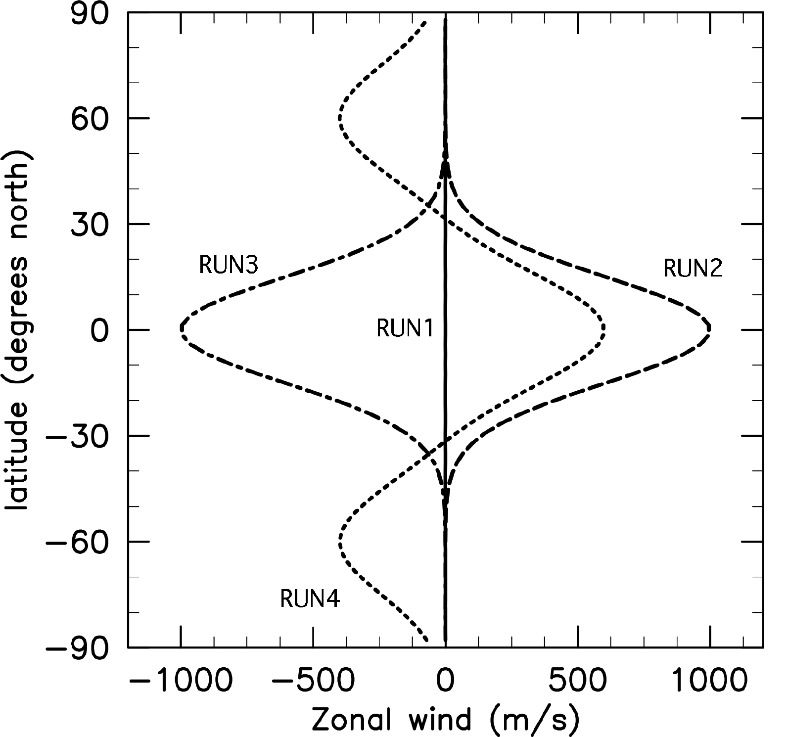
Figure 1: Initial conditions for simulations RUN1 (—), RUN2 (- - -), RUN3 ($-\,\cdot\,-$), and RUN4 ($\cdots$). The height-independent, zonally-symmetric, eastward velocities, $u(\lambda,\phi,\eta,0)=u_{0}(\phi)$, are shown.

To examine the robustness of evolved flow states to organized initial flow configurations, we have performed simulations with a wide range of initial conditions. The conditions from four of those runs (labeled RUN1–RUN4) are shown in Figure 1. In all the runs presented, the setup is identical—except for the initial flow configuration. The physical and numerical parameters/conditions are given in Tables 1 and 2, respectively.

RUN1 is initialized with a small, random perturbation introduced in the flow. Specifically, values of $u$ and $v$ are drawn from a Gaussian random distribution centered on zero with a standard deviation of 0.05 m s^-1. RUN2 is initialized with a zonally-symmetric, eastward equatorial jet of the following form:

$$u_{0}(\phi)\ =\ U\exp\left\{\frac{(\phi-\phi_{0})^{2}}{2\sigma^{2}}\right\},$$ (5)

where $u(t\!=\!0)\,=\,u_{0}$, $U=1000$ m s^-1, $\phi_{0}=0$, and $\sigma=\pi/12$. RUN3 is initialized with a westward equatorial jet described by equation (5), with $U=-1000$ m s^-1, $\phi_{0}=0$, and $\sigma=\pi/12$. RUN4 is initialized with a flow containing three jets. Note that the condition for RUN4 is very similar to the zonal average of the wind field of RUN1 at 50 planetary rotations. The jet profiles presented in Figure 1 are independent of height, as well as longitude.

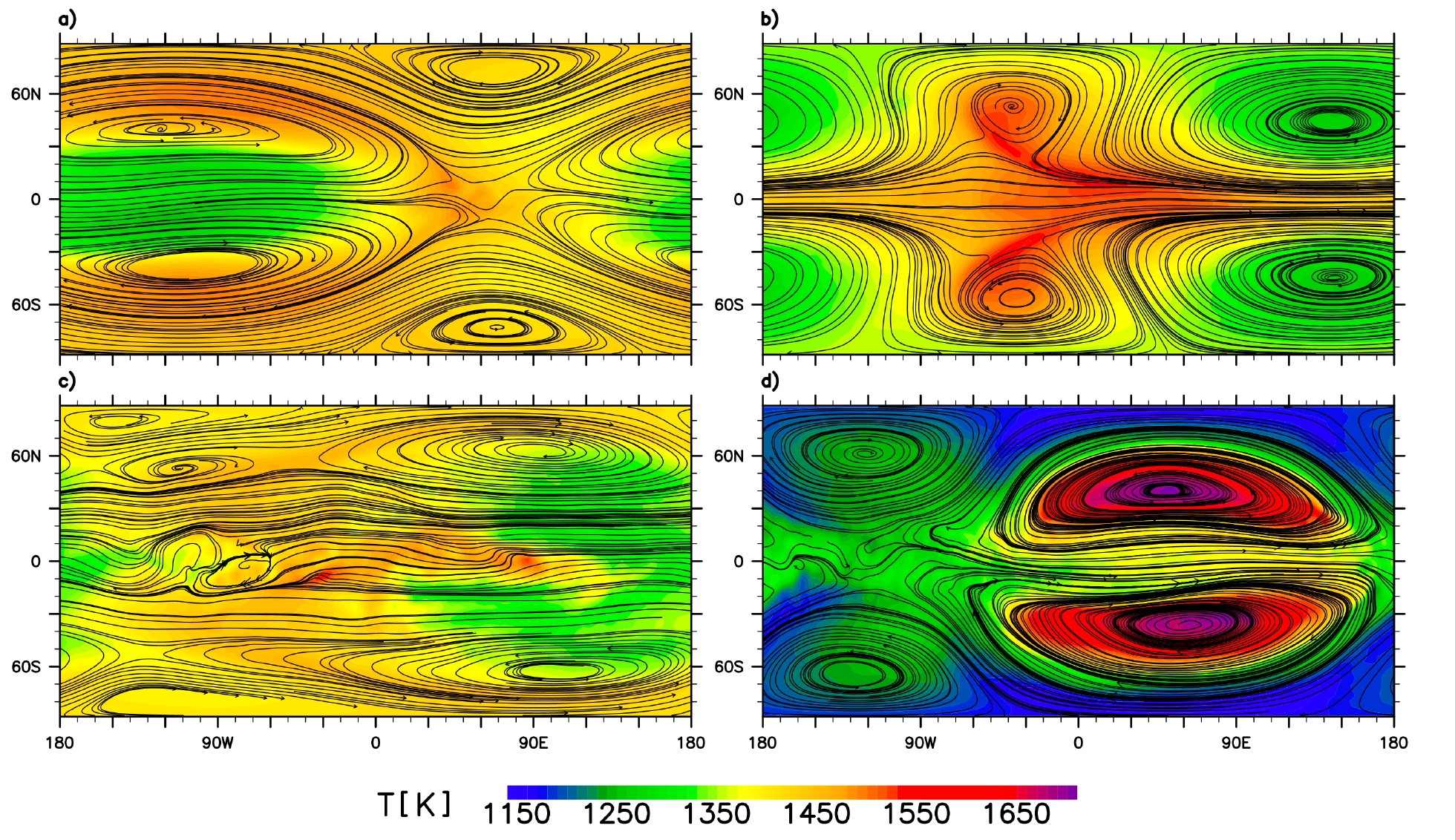
Figure 2: Temperature (color map) and flow (streamlines) fields at $t=40\,\tau_{p}$, near the $p\sim 900$ mbar level, for RUN1 (a), RUN2 (b), RUN3 (c), and RUN4 (d). The fields are shown in cylindrical-equidistant projection centered at the equator. The four simulations are set up identically, except for the initial wind field. The location and size of vortices, and the associated temperature patterns, strongly depend on the initial wind configuration.

Figure 2 shows the temperature and flow fields of the four runs at $t/\tau_{p}=40$ (or $t/\tau_{\rm th}\approx\!14$). The fields near the 900 mbar pressure level are shown. [Recall that the $\eta$ level-surfaces of our model are functions of pressure, as described by equation (2).] The figure illustrates the major point of this paper: given different initial states, there are clear, qualitative (as well as quantitative) differences between the different runs. Qualitatively, there are some common features. For example, most of the runs exhibit a coherent quadrupole flow structure—two large cyclonic and anti-cyclonic vortex-pairs straddling the equator. However, the location of an individual vortex is different in the runs—as is the temperature pattern. In RUN3, a distinct quadrupole pattern is not present but there are more vortices in this run compared to the other runs. The temperature distributions are different because they are strongly linked to the flow. Consequently, the minimum-to-maximum temperature ranges vary from a moderately large 550 K (RUN4) to only about 200 K (RUN3) in the figure.

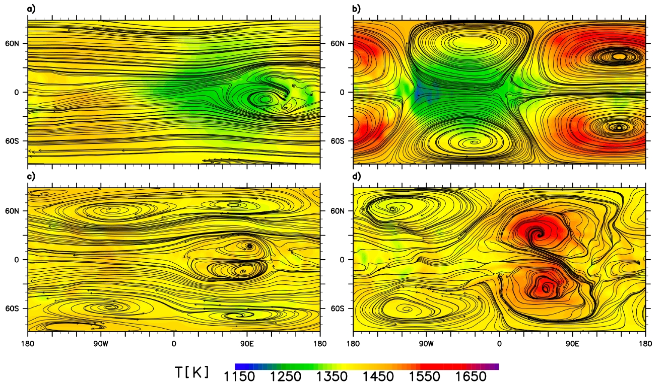
Figure 3: Temperature (color map) and flow (streamlines) fields at $t=40\,\tau_{p}$, near the $p\approx$ 85 mbar level, for the same four simulations as shown in Figure 2: RUN1 (a), RUN2 (b), RUN3 (c) and RUN4 (d). The sensitivity to the initial wind state is present throughout all heights in the atmosphere.

The behavior just described is not restricted to a single altitude. Figure 3 shows the fields corresponding to those presented in Figure 2, but at a higher altitude ($p\approx 85$ mbar pressure level). Comparison of Figures 2 and 3 illustrates the structural differences in 3-D (vertical), as well as in 2-D (horizontal). In RUN2 and RUN4, the large-scale vortices are strongly aligned, forming columns through most of the height extent of the modeled atmosphere; that is, the flow is strongly barotropic. In the other two runs, the flow is not vertically aligned throughout in large parts of the modeled atmosphere—and, therefore, the flow is baroclinic. The two figures also point to the corresponding strong difference in 3-D temperature distributions, associated with the flow structures.

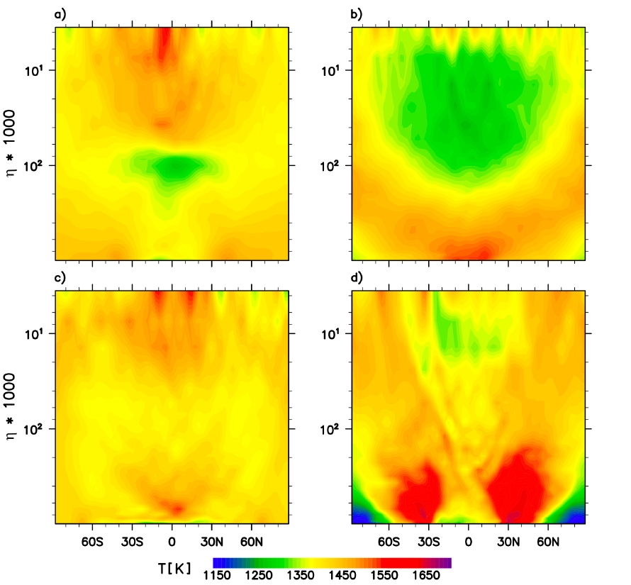
Figure 4: Snapshots of temperature vertical cross-section at the sub-stellar longitude, at $t=40\,\tau_{p}$, for the four simulations presented in Figure 2: RUN1 (a), RUN2 (b), RUN3 (c) and RUN4 (d). The vertical temperature structure is strongly sensitive to the initial flow state, and usually contains an inversion.

This is more clearly seen in Figure 4. The figure shows the vertical (height-latitude) cross-section of the temperature at 0 degrees (sub-stellar) longitude from the runs presented in Figures 2 and 3. In Figure 4, the hottest and coldest regions are at different locations in all the runs. Near the equator, RUN1 exhibits a strong temperature inversion, while RUN2 and RUN4 do not. In addition, RUN2 and RUN4 exhibit generally strong decreases in temperature with height, while the others do not. As can be seen, the degree of temperature mixing varies strongly in the vertical direction among the runs—from $\sim\!200$ K contrast (RUN3) to $\sim\!500$ K contrast (RUN4). In general, the vertical structure is of low order, containing usually a single inversion. In our study, some form of inversion appears to be a generic feature.

Preliminary steady state analysis of the primitive equations suggests that the basic behavior described above is due to the way in which the applied, $(s,n)=(1,1)$, forcing projects onto the normal modes of the planetary atmosphere; here, $s$ is the zonal wavenumber and $n$ is the total (sectoral) wavenumber of the spectral harmonics. In particular, a normal mode decomposition of the atmosphere into the vertical structure and Hough functions (e.g., Chapman & Lindzen, 1970; Longuet-Higgins, 1967) indicates that the forcing projects mostly onto low-order baroclinic modes, when the initial state is at rest. In contrast, when the initial state contains large-scale jets, the forcing projects more strongly on the barotropic mode, compared to the runs started from rest. Similar behavior has been observed in studies of the Earth’s troposphere under tropical forcing (e.g., Geisler & Stevens, 1982; Lim & Chang, 1983). A more detailed study of coupling between forcing and normal modes is currently being performed and will be described elsewhere.

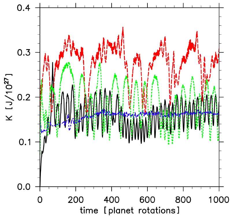
Figure 5: Time series of total kinetic energy, integrated over the domain, for RUN1 (black —), RUN2 (red – – –), RUN3 (blue $-\,\cdot\,-$), and RUN4 (green - - -).

Furthermore, it is important to note that all of the above features, both dynamical and thermal, can vary in time. All of these features are important for observations (e.g., Knutson et al., 2007) and spectral modeling (e.g., Tinetti et al., 2007). A thorough study of the long-time evolution (over 1000 planetary rotations, or more than $330~{}\tau_{\rm{th}}$) of the runs reveals a fundamental difference in their temporal behavior as well. For example, the flow pattern in RUN2 is characterized by two vertically aligned vortex columns in each hemisphere that translate longitudinally around the poles. The temperature in the upper altitude region is more strongly coupled to the flow than it is in the lower altitude regions. The flow pattern in RUN4 is also a set of vertically aligned vortex columns, but the columns oscillate in the east-west direction. The patterns in RUN1 and RUN3 are more complex, exhibiting a mixture of vortex splitting and merger and stationary states at different altitude levels. Figure 5, which shows a time series of the total kinetic energy, gives a quantitative measure of the different temporal behavior of the simulations.

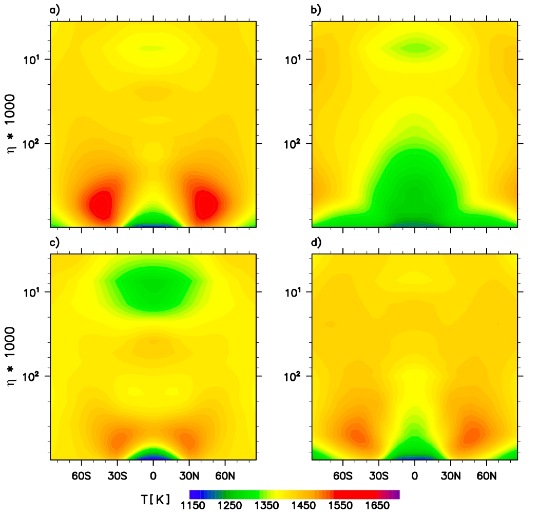
Figure 6: Temperature vertical cross-section at an arbitrary longitude ($\lambda=135^{\circ}$), averaged over 450 planetary rotations (150 thermal drag times), for the four simulations presented in Figure 2: RUN1 (a), RUN2 (b), RUN3 (c) and RUN4 (d). The difference in the temperature structure is independent of long time-averaging and is not due to a phase shift in a quasi-periodic evolution.

When the flow field is time-averaged over a long period, the time-mean state is also significantly sensitive to the initial flow. This can be seen in Figure 6, which shows temperature cross-sections at an arbitrary longitude ($\lambda=135^{\circ}$), averaged over 450 planetary rotations (planet day 300 to 750). The figure clearly shows that the variability observed is not simply a result of a phase shift in a quasi-periodic evolution. The flow and temperature structures in each run are fundamentally different from one another.

Interestingly, the full range of flow and temperature behavior described above has been previously captured qualitatively, using the one-layer equivalent-barotropic model (Cho et al., 2008). The equivalent-barotropic equations are a reduced, vertically-integrated version of the full primitive equations used in this study (Salby, 1989). In many situations, the reduced model can be fruitfully used to study the dynamics of the full model by varying the Rossby deformation radius to represent different heights (or temperatures) of the full multi-layer model (e.g., Cho et al., 2008; Scott & Polvani, 2008), and this also appears to be the case for hot extrasolar planets.

3.2 Extreme Sensitivity: Small Stirring

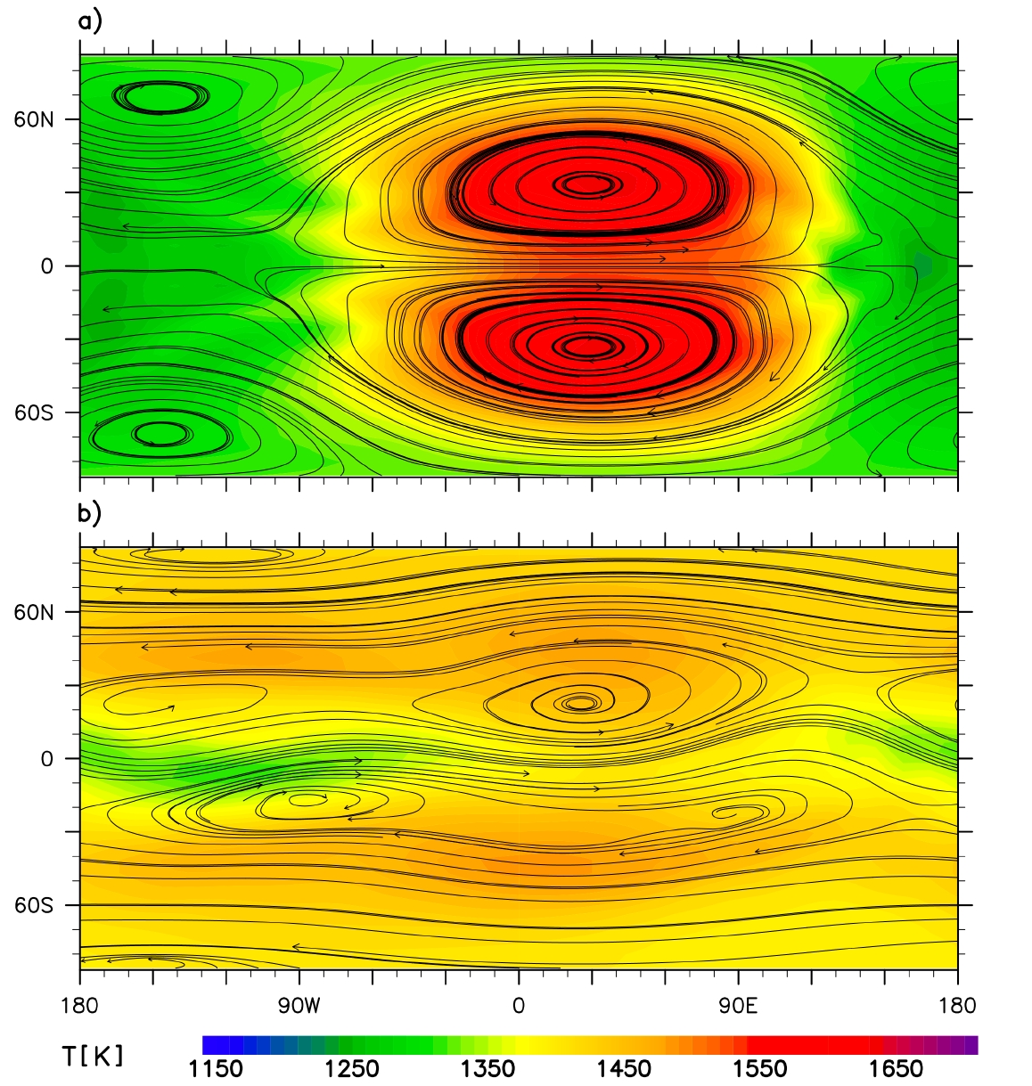
Figure 7: Temperature (color map) and flow (streamlines) fields after 1000 planetary rotations, at the $p\sim 420$ mbar level, for two simulations differing only by small deviations in the initial wind. The top panel shows the result of a simulation started from rest, while the bottom panel is from a simulation started with a small perturbation. Note the clear asymmetry in the north-south direction, which only appears when the small perturbations are present in the initial state.

As might be expected from general nonlinear dynamics theory, in fact the evolution can be strongly sensitive to small differences in the initial flow state. This is illustrated in Figure 7. There, two simulations are presented (panels a and b), which are identical in all respects except for a minute difference in the initial flow. The simulation in the top panel (RUN5) is started from rest. In contrast, the simulation in the bottom panel (RUN1) is started with a small perturbation: the initial values of $u$ and $v$ at each grid point are set to a Gaussian random distribution, centered on zero with a standard deviation of 0.05 m s^-1. Note that the maximum initial wind perturbation magnitude is only about 0.02% of the typical root mean square flow speed in the frames shown ($\sim$ 500 m s^-1).

The two panels in Figure 7 show temperature and flow distributions after $t/\tau_{p}=1000$ (or $t/\tau_{\rm th}\approx 333$) at the $p\sim 420$ mbar level. The distributions in the two panels are clearly different. At times they may look more similar than shown here, but in general that is not the case. The two runs generally show a different temporal behavior. Note that in Figure 7a, there is a high degree of hemispheric symmetry, particularly in the north-south direction. In contrast, Figure 7b shows a clear asymmetry in both the north-south and east-west direction. The small asymmetry in Figure 7a is entirely due to machine precision and is not physical, since there is no way to break the symmetry in the setup of the run. Therefore, not surprisingly, some mechanism for inducing a noticeable symmetry breaking is necessary. The salient point here is, however, that even a tiny perturbation can lead to a marked difference in the flow and temperature distributions, even at relatively early integration times.

3.3 Robustness: Additional Parameter Variations

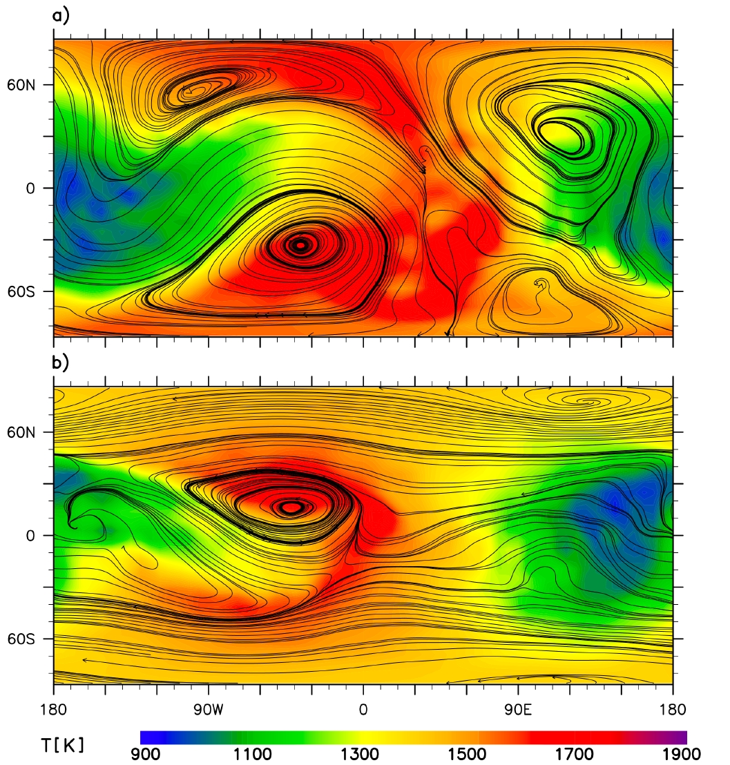
Figure 8: Snapshots of temperature fields (color coded) with streamlines overlaid. Fields at the $p\sim$ 900 mbar level are shown at t = 1000 planetary rotations, for two simulations (RUN6 and RUN7); the thermal drag time is 0.5 planetary rotations (42 hours) in these runs. The only difference between the simulations is the initial wind state. The top panel shows the result of a simulation started with only a small perturbation and the bottom panel is from a simulation started with a westward jet. The sensitivity to the initial flow state is still present for this small value of the thermal drag time (cf., RUNS 1–4).

It is important to understand that the dependence on the initial flow state is robust and the behavior is not limited only to the parameters, and the ranges, discussed thus far. The dependence has been verified for numerous model parameters and ranges. For example, Figure 8 shows that the strong dependence on the initial wind exists for much shorter $\tau_{\rm th}$, despite the strong forcing such drag times entail. In this case, $\tau_{\rm th}/\tau_{p}=0.5$. The upper panel is from RUN6 and the lower panel is from RUN7. The former run is initialized with only small stirring and no organized jet. In contrast, the latter run is initialized with a westward equatorial jet, identical to the setup of RUN3. At the shown time and height, there are clear differences between the flow and temperature patterns of the two simulations. The coldest area is advected east of the anti-stellar point in RUN6, but west of the anti-stellar point in RUN7. Furthermore, all the vortices have different locations. In RUN7, there is a fairly zonally symmetric jet at high latitudes, leading to a much more homogenized temperature distribution above the mid-latitudes than in RUN6.

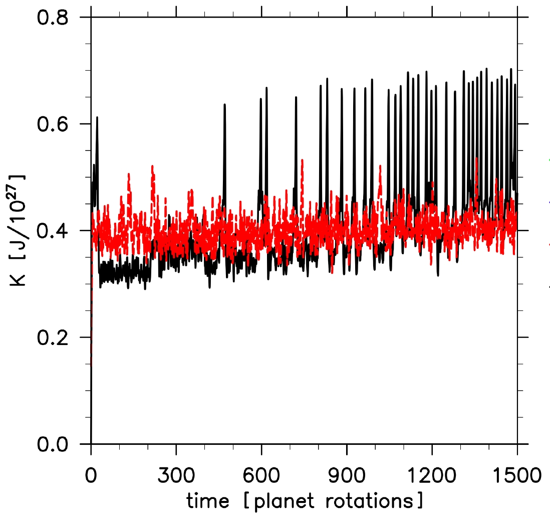
Figure 9: Time series of total kinetic energy, integrated over the domain, for RUN6 (black —) and RUN7 (red – – –).

While a weaker difference might be expected in this case, based on other studies (e.g., Cooper & Showman 2005), the sensitivity is unabated in our simulations. And, this holds for the long time average behavior as well. For a time mean over 300 rotations (e.g., planet days 1200 to 1500), at the level shown in Figure 8, the location of the coldest region differs by 40 degrees in longitude between the two simulations shown in the figure. Figure 9 shows a time series of the total kinetic energy in the two simulations, revealing their different evolution. Even after integrating for a very long time (15,000 rotations), we have checked that the differences between RUN6 and RUN7 are still present. Note that this is a much longer integration time than that reported in any published studies of close-in planet circulation thus far. However, the flow at such long times is inexorably affected by cumulative numerical dissipation and phase errors and the result obtained should not be taken too literally (e.g., Canuto et al., 1988).

In addition, we have studied the dependence when the initial jet contains a vertical shear–i.e., the jet distribution is baroclinic. Simulations have been initialized with an eastward jet, which has zero magnitude at the bottom and increases linearly with height so that the lateral flow distribution in the top layer of the model is identical to that in RUN2. In the baroclinic case, vortex columns evolve that extend throughout most of the atmosphere, as in RUN2. However, unlike in RUN2, the temperature structure here is also strongly barotropic. This appears to be related to the way the forcing projects onto the free modes of the system, as described in section 3.1.

As alluded to in section 2.1, the timescale of the fastest motions admitted by equations (1) with the given boundary condition is $\sim\!40$ minutes, for the planetary physical parameters used in this work. Hence, a forcing with timescales of the same order or smaller is not entirely physically self-consistent with the use of equations (1). Notably, such forcing introduces numerical difficulties. For the physically unrealistic drag time of $\tau_{\rm th}$ = 1 hour, for which excessive numerical dissipation is required to prevent the code from blowing up or being inundated with numerical noise, the temperature evolution is only mildly sensitive to the initial condition, at long-time integrations. However, when such short drag times are only applied over a limited range in pressure—i.e., $\tau_{\rm th}$ is allowed to vary with $\eta$— the sensitivity to the initial condition is present even after long time integrations (7000 planet days).

4 Conclusion

In this paper, we have shown that in a generic general circulation simulation of a tidally synchronized planet, the flow and temperature distributions depend strongly on the initial state. In all simulations initialized with a different jet configuration, large scale coherent vortices are formed; but, their location, size, and number varies, depending on the initial wind. The temperature distribution is relatively homogenized by the flow, compared to the large temperature contrast in the forcing equilibrium temperature profile. But the degree of mixing, as well as locations of temperature extremes vary between differently initialized simulations. The time variability of the atmosphere—i.e. how vortices and associated temperature patterns move around the planet or whether they stay at fixed positions—varies depending on the initial wind.

The Newtonian drag scheme used in this study is idealized and the “correct” parameters to use in the set-up are unknown, with many choices possible. Explorations of different parts of the parameter space will be presented elsewhere. Here, we have chosen the set-up to capture, as cleanly as possible, the effects of the initial flow in a regime of parameter space plausibly relevant for hot Jupiters with strong zonally-asymmetric forcing. We have found that the strong dependence on the initial wind is valid for a wide range of thermal drag times ($\tau_{\rm th}$ = 0.5–10 planet days) and with T21, T42, and T85 resolutions. Some reduction in the sensitivity is sometimes observed for the very small $\tau_{\rm th}$ and long time integration simulations, which require large numerical dissipation to prevent the fields from being dominated by small scale noise. This situation is, however, not physically realistic and numerically suspect.

The strong dependence on initial wind has implications for the use of general circulation models for interpretation of observations of extrasolar planet atmospheres. These results underline that, while numerical circulation models of the kind employed here are useful for studying plausible mechanisms and flow regimes, they are currently unsuitable for making “hard” predictions—such as exact locations of temperature extremes on a given planet.

Appendix A Appendix

Table 3 presents the $A$ and $B$ coefficients of equation (2) in §2.2. Note that, as defined, each $\eta$-surface can span across a range of $p$-surfaces.

Table 1: Physical Parameters

Planetary rotation rate	$\Omega$	2.1$\times$10-5	s-1
Planetary radius	$R_{p}$	108	m
Gravity	$g$	10	m s-2
Specific heat at constant pressure	$c_{p}$	1.23$\times$104	J kg-1 K-1
Specific gas constant	$R$	3.5$\times$103	J kg-1 K-1
Mean equilibrium temperature	$T_{m}$	1400	K
Equilibrium substellar temperature	$T_{D}$	1900	K
Equilibrium antistellar temperature	$T_{N}$	900	K
Initial temperature	$T_{0}$	1400	K

Table 2: Summary of Runs Discussed

RUN	Initial Flow	$\tau_{\rm th}$ [$2\pi/\Omega$]	$N$	$\nu$ [1021 m4 s-1]
1	small noise	3	42	1
2	eastward jet	3	42	1
3	westward jet	3	42	1
4	three jets	3	42	1
5	zero winds	3	42	1
6	small noise	0.5	21	10
7	westward jet	0.5	21	10

Note. — $\tau_{\rm th}$ is the thermal drag timescale, $N$ is the spectral truncation wavenumber, and $\nu$ is the superviscosity coefficient. All the runs have Robert-Asselin filter coefficient $\epsilon$ = 0.06. In the T42 runs the timestep is $\Delta t$ = 120 s, but for T21 resolution $\Delta t$ = 240 s.

Table 3: Vertical Coordinate Coefficients

Level Surface Index	A$\times 10^{3}$	B$\times 10^{3}$
0	2.2	0
1	4.9	0
2	9.9	0
3	18.1	0
4	29.8	0
5	44.6	0
6	61.6	0
7	78.5	0
8	77.3	15.0
9	75.9	32.8
10	74.2	53.6
11	72.3	78.1
12	70.0	106.9
13	67.3	140.9
14	64.1	180.8
15	60.4	227.7
16	56.0	283.0
17	50.8	347.9
18	44.7	424.4
19	37.5	514.3
20	29.1	620.1
21	20.8	723.5
22	13.3	817.7
23	7.1	896.2
24	2.5	953.5
25	0	985.1
26	0	1000.0

References

- Asselin (1972) Asselin, R. 1972, Mon. Wea. Rev., 100, 487
- Burrows et al. (2007) Burrows, A., Hubeny, I., Budaj, J., Knutson, H. A., and Charbonneau, D. 2007, ApJ, 668, L171
- Canuto et al. (1988) Canuto, C., Hussaini, M.Y., Qarteroni, A., and Zang, T.A. 1988, Spectral Methods in Fluid Dynamics (New York, NY: Springer)
- Chapman & Lindzen (1970) Chapman, S. and Lindzen, R.S. 1970, Atmospheric Tides (New York, NY: Gordon and Breach)
- Cho et al. (2003) Cho, J. Y-K., Menou, K., Hansen, B. M. S., and Seager, S. 2003, ApJ, 587, L117
- Cho et al. (2008) Cho, J.Y-K., Menou, K., Hansen, B.M.S., and Seager, S. 2008, ApJ, 675, 817
- Cho (2008) Cho, J.Y-K. 2008, Phil. Trans. R. Soc. A, 366, 4477
- Collins et al. (2004) Collins, W.D. et al. 2004, NCAR/TN-464+STR
- Cooper & Showman (2005) Cooper, C.S. and Showman, A.P. 2005, ApJ, 629, 45L
- Dobbs-Dixon & Lin (2008) Dobbs-Dixon, I. and Lin, D.N.C. 2008, ApJ, 673, 513
- Dritschel et al. (2007) Dritschel, D.G., Tran, C.V. and Scott, R.K. 2007, J. Fluid Mech., 591, 379
- Geisler & Stevens (1982) Geisler, J.E. and Stevens, D.E. 1982, Quart. J. Roy. Meteor. Soc., 108, 87
- Eliasen et al. (1970) Eliasen, E., Mechenhauer, B., and Rasmussen, E. 1970, Copenhagen Univ., Inst. Teoretisk Meteorologi, Tech. Rep. 2
- Holton (2004) Holton, J. R. 2004, Introduction to Dynamical Meteorology (Burlington, MA: Academic Press)
- Knutson et al. (2007) Knutson, H., et al., 2007, Nature, 447, 183
- Knutson et al. (2008) Knutson, H. A., Charbonneau, D., Allen, L. E., Burrows, A., and Megeath, S. T. 2008, ApJ, 673, 526
- Langton & Laughlin (2007) Langton, J. and Laughlin, G. 2007, ApJ, 657, 113L
- Lim & Chang (1983) Lim, H. and Chang, C.P. 1983, J. Atmos. Sci., 40, 1897
- Longuet-Higgins (1967) Longuet-Higgins, M.S. 1967, Phil. Trans. R. Soc. A, 269, 511
- Menou & Rauscher (2009) Menou, K. and Rauscher, E. 2009, ApJ, 700, 887
- Orszag (1970) Orszag, A. 1970, J. Atmos. Sci., 27, 890
- Pedlosky (1987) Pedlosky, J. 1987, Geophysical Fluid Dynamics (New York, NY: Springer-Verlag)
- Robert (1966) Robert, A. 1966, J. Meteorol. Soc. Japan, 44, 237
- Salby (1989) Salby, M. L., 1989, Tellus, 41A, 48
- Scott & Polvani (2008) Scott, R. K. and Polvani, L.M. 2008, Geophys. Res. Lett., 35, L24202
- Showman & Guillot (2002) Showman, A. P. and Guillot, T. 2002, A&A, 385, 166
- Showman et al. (2008) Showman, A.P., Cooper, C.S., Fortney, J.J., and Marley, M.S. 2008, ApJ, 682, 559
- Showman et al. (2008) Showman, A.P., Menou, K., and Cho, J. Y-K. 2008, in ASP Conf. Ser. 398, Extreme Solar Systems, ed. D. Fischer et al. (San Francisco, CA: ASP)
- Tinetti et al. (2007) Tinetti, G. et al., 2007, Nature, 448, 169