Deterministic flows of order-parameters in stochastic processes of quantum Monte Carlo method

Abstract

In terms of the stochastic process of quantum-mechanical version of Markov chain Monte Carlo method (the MCMC), we analytically derive macroscopically deterministic flow equations of order parameters such as spontaneous magnetization in infinite-range ($d(=\infty)$-dimensional) quantum spin systems. By means of the Trotter decomposition, we consider the transition probability of Glauber-type dynamics of microscopic states for the corresponding $(d+1)$-dimensional classical system. Under the static approximation, differential equations with respect to macroscopic order parameters are explicitly obtained from the master equation that describes the microscopic-law. In the steady state, we show that the equations are identical to the saddle point equations for the equilibrium state of the same system. The equation for the dynamical Ising model is recovered in the classical limit. We also check the validity of the static approximation by making use of computer simulations for finite size systems and discuss several possible extensions of our approach to disordered spin systems for statistical-mechanical informatics. Especially, we shall use our procedure to evaluate the decoding process of Bayesian image restoration. With the assistance of the concept of dynamical replica theory (the DRT), we derive the zero-temperature flow equation of image restoration measure showing some ‘non-monotonic’ behaviour in its time evolution.

1 Introduction

In Bayesian statistics and statistical inference within the framework, to evaluate the expectation of microscopic labels (such as ‘pixels’ or ‘bits’) over the posterior distribution of these microscopic states or to calculate the marginal probability is very important procedure to solve various problems in the research field of ‘massive’ probabilistic information processing [1]. For most of the cases, it is very hard for us to carry out the task except for several limited cases of solvable probabilistic models. Recently, to overcome the difficulty, deterministic approaches based on mean-field approximation including the belief-propagation succeeded in dealing with the problems efficiently [2, 3].

On the other hand, in a lot of research fields, the Markov chain Monte Carlo method (the MCMC) has been widely used to calculate these expectations or to make marginal distributions by sampling the important states that contribute effectively to the macroscopic quantities [4]. Generally speaking, the MCMC takes a long time to wait until the Markovian stochastic process starts to generate the microscopic states from well-approximated posterior distribution. Especially, for some classes of probabilistic models which are categorized in the so-called spin glasses [5, 6, 7], the time consuming is sometimes very serious to make attempt to proceed the desired information processing within a realistic time. However, even for such cases, various improvements based on several important concepts have been proposed and succeeded in carrying out the numerical calculations [8, 9]. From the view point of statistical physics, transitions between microscopic states are controlled by a specific hyper-parameter, namely, ‘temperature’ of the system and by cooling the temperature slowly enough during the Markovian stochastic process, one can get the lowest energy states efficiently. This type of optimization tool based on ‘thermal fluctuation’ is referred to as simulated annealing [10, 11].

Recently, the simulated annealing has been extended to the quantum-mechanical version. This new type of simulated annealing called as quantum annealing [12, 13, 14, 15, 16] is based on the adiabatic theorem of the quantum system that evolves according to Schr$\ddot{\rm o}$dinger equations. To use the quantum annealing, or more generally, to utilize the quantum fluctuation for combinatorial optimization problems or massive information processing dealing with a huge number of particles such as image restoration or error-correcting codes, the approach by solving the Schr$\ddot{\rm o}$dinger equations is apparently limited and we should look for different ways to simulate the quantum systems.

As the most effective and efficient way, the quantum Monte Carlo method [17] was established. The method is based on the following Suzuki-Trotter decomposition for non-commutative two operators ${\cal A}$ and ${\cal B}$ :

$${\rm tr}\,{\exp}\left({\cal A}+{\cal B}\right) = \lim_{M\to\infty}{\rm tr}\left({\exp}\left(\frac{{\cal A}}{M}\right){\exp}\left(\frac{{\cal B}}{M}\right)\right)^{M}$$ (1)

Namely, the $d$-dimensional quantum system is mapped to the corresponding $(d+1)$-dimensional classical spin systems. This approach is very powerful and a lot of researches have succeeded in exploring the quantum phases in strongly correlated quantum systems. However, when we simulate the quantum system at zero temperature in which quantum effect is essential, we encounter some technical difficulties although several sophisticated algorithms were proposed [18]. From the view point of information science, it is very informative for us to evaluate the process of information processing and if one seeks to utilize the quantum fluctuation to solve the problems, we should use the ‘zero-temperature dynamics’. For this purpose, it seems that we need some tractable ‘bench mark tests’ to investigate the ‘dynamical process’ of information processing such as quantum annealing by using quantum fluctuation at zero temperature.

In classical system, Coolen and Ruijgrok [19] proposed a way to derive the differential equations with respect to order-parameters of the system from the microscopic master equations for the so-called Hopfield model [20] as an associative memory in which a finite number of patterns are embedded. The procedure was extended by Coolen and Sherrington [21], Coolen, Laughton and Sherrington [22] to more complicated spin systems categorized in the infinite-range (or mean-field) models including the Sherrington-Kirkpatrick spin glasses [23]. The so-called dynamical replica theory (DRT) was now established as a strong approach to investigate the dynamics in the classical disordered spin systems . On the considering the matter, it seems to be very important for us to extend their approach to quantum systems evolving stochastically according to the quantum Monte Carlo dynamics.

In this paper, in terms of the stochastic process of quantum-mechanical version of Markov chain Monte Carlo method, we analytically derive macroscopically deterministic flow equations of order parameters such as spontaneous magnetization in infinite-range ($d(=\infty)$-dimensional) quantum spin systems. By means of the Trotter decomposition, we consider the transition probability of Glauber-type dynamics of microscopic states for the corresponding $(d+1)$-dimensional classical system. Under the static approximation, differential equations with respect to macroscopic order parameters are explicitly obtained from the master equation that describes the microscopic-law. In the steady state, we show that the equations are identical to the saddle point equations (equations of states) for the equilibrium state of the same system. We easily find that the equation for the dynamical Ising model is recovered in the classical limit. We also check the validity of the static approximation by computer simulations for finite size systems and discuss several possible extensions of our approach to disordered spin systems for statistical-mechanical informatics [24]. Especially, we shall use our procedure to evaluate the decoding process of Bayesian image restoration [25, 26, 27, 28, 29]. With the assistance of the concept of dynamical replica theory (the DRT) [21, 22], we derive the zero-temperature flow equation of image restoration measure, namely, overlap function between a given original image and the degraded one, showing some ‘non-monotonic’ behaviour in its time evolution.

This paper is organized as follows. In Section 2, we explain our formulation to describe the deterministic flow equation from master equation for a simplest quantum spin system. In Section 3, we apply our approach to evaluate the decoding process of Bayesian image restoration. Some ‘non-monotonic’ behaviour in time evolution of image restoration measure is observed by the analysis of flow equations. The last section contains some remarks.

2 The model system and formulation

In this section, we derive the differential equations with respect to several order parameters for a simplest quantum spin system, namely, a class of the infinite range transverse Ising model [30, 31] described by the following Hamiltonian:

$$H = -\frac{1}{N}\sum_{i,j=1}^{N}J_{ij}\sigma_{i}^{z}\sigma_{j}^{z}-h\sum_{i=1}^{N}\tau_{i}\sigma_{i}^{z}-\Gamma\sum_{i=1}^{N}\sigma_{i}^{x}.$$ (2)

where $\sigma_{i}^{z}$ and $\sigma_{i}^{x}$ denote the Pauli matrices given by

$$\sigma_{i}^{z} = \left(\begin{array}[]{cc}1&0\\ 0&-1\end{array}\right),\,\,\,\,\sigma_{i}^{x}=\left(\begin{array}[]{cc}0&1\\ 1&0\end{array}\right).$$

It should be noticed that from the view point of Bayesian statistics, the above Hamiltonian corresponds to the logarithm of the posterior distribution. For various choices of parameters $\{J_{ij}\},h$ and $\{\tau\}$, one can model the problem of information processing appropriately. For instance, for the choice of $J_{ij}=J,h\neq 0$, the above Hamiltonian describes image restoration [26, 28, 29] from a given set of degraded images $\mbox{\boldmath$\tau$}=(\tau_{1},\cdots,\tau_{N})$ by means of Markov random fields. For $J_{ij}\neq 0,h=0$, it corresponds to the logarithm of the posterior of the Sourlas codes [32, 33] sending the parity check of two-body interactions $\xi_{i}\xi_{j}\,\,\,\forall(i,j)$ through the binary symmetric channel (BSC). For the Sherrington-Kirkpatrick model [23], we may choose $J_{ij}$ obeying the Gaussian with $J_{0}$ mean and $\tilde{J}^{2}$ variance. Especially, for the choice of the so-called Hebb rule $J_{ij}=\sum_{\mu=1}^{\alpha N}\xi_{i}^{\mu}\xi_{j}^{\mu},h=0$, it becomes energy function of the Hopfield model [20] in which extensive number of patterns (loading rate $\alpha$) are embedded.

In this section, we focus on the simplest case of $J_{ij}=J>0,h=0$ ferromagnetic transverse Ising model [34, 35]. Let us start our argument from the effective Hamiltonian which is decomposed by the Suzuki-Trotter formula (1).

$$\beta H = -\sum_{k=1}^{M}\sum_{i=1}^{N}\beta\phi_{i}(\mbox{\boldmath$\sigma$}_{k}:\sigma_{i}(k+1))\sigma_{i}(k)=-\frac{\beta J}{MN}\sum_{k,ij}\sigma_{i}(k)\sigma_{j}(k)-B\sum_{k,i}\sigma_{i}(k)\sigma_{i}(k+1)$$ (4)

where $k$ means the Trotter index and $M$ denotes the number of the Trotter slices. We also defined the parameter $B$ as $B\equiv(1/2)\log\coth(\beta\Gamma/M)$ and a microscopic spin state on the $k$-th Trotter slice by $\mbox{\boldmath$\sigma$}_{k}\equiv(\sigma_{1}(k),\sigma_{2}(k),\cdots,\sigma_{N}(k)),\,\sigma_{i}(k)\in\{+1,-1\}$.

2.1 The Glauber dynamics and its transition probability

In the expression of the effective Hamiltonian (4), $\beta\phi_{i}(\mbox{\boldmath$\sigma$}_{k},\sigma_{i}(k+1))$ is a local field on the cite $i$ in the $k$-th Trotter slice, which is explicitly given by

$$\beta\phi_{i}(\mbox{\boldmath$\sigma$}_{k}:\sigma_{i}(k+1)) = \frac{\beta J}{MN}\sum_{j}\sigma_{j}(k)+B\sigma_{i}(k+1).$$

It should be noticed that the effective Hamiltonian (4) is a classical system under the Trotter decomposition. Therefore, the quantum Monte Carlo dynamics should be described by the Glauber-type stochastic update rule whose transition probability is explicitly written by

$$w_{i}(\mbox{\boldmath$\sigma$}_{k}) = \frac{1}{2}\left[1-\sigma_{i}(k)\tanh(\beta\phi_{i}(\mbox{\boldmath$\sigma$}_{k}:\sigma(k+1)))\right].$$

Namely, this means that

$$\sigma_{i}(k) = \left\{\begin{array}[]{ccc}+1&\mbox{with prob.}&\frac{{\exp}[\beta\phi_{i}(\mbox{\boldmath$\sigma$}_{k}:\sigma_{i}(k+1))]}{{\exp}[\beta\phi_{i}(\mbox{\boldmath$\sigma$}_{k}:\sigma_{i}(k+1))]+{\exp}[-\beta\phi_{i}(\mbox{\boldmath$\sigma$}_{k}:\sigma_{i}(k+1))]}\\ -1&\mbox{with prob.}&\frac{{\exp}[-\beta\phi_{i}(\mbox{\boldmath$\sigma$}_{k}:\sigma_{i}(k+1))]}{{\exp}[\beta\phi_{i}(\mbox{\boldmath$\sigma$}_{k}:\sigma_{i}(k+1))]+{\exp}[-\beta\phi_{i}(\mbox{\boldmath$\sigma$}_{k}:\sigma_{i}(k+1))]}\end{array}\right.$$ (7)

Obviously, in the classical limit, namely, when $B$ goes to infinity as $\Gamma\to 0$ and $\phi_{i}(\mbox{\boldmath$\sigma$}_{k}:\sigma_{i}(k+1))\sim B\sigma_{i}(k+1)$, $\sigma_{i}(k)$ is identical to $\sigma_{i}(k+1)$ with probability $1$. Thus, for small $\Gamma$, we have $\mbox{\boldmath$\sigma$}_{k}=\mbox{\boldmath$\sigma$}_{k+1}$ with a relatively high probability. In this sense, we can regard the term $B\sigma_{i}(k+1)$ as an ‘external field’ from the nearest Trotter slice $k+1$. Here we use the periodic boundary condition for the Trotter direction, that is, $\mbox{\boldmath$\sigma$}_{1}=\mbox{\boldmath$\sigma$}_{M+1}$.

2.2 The master equation

Then, the master equation for the probability of the microscopic states on the $k$-th Trotter slice $p_{t}(\mbox{\boldmath$\sigma$}_{k})$ is written by

$$\frac{dp_{t}(\mbox{\boldmath$\sigma$}_{k})}{dt} = \sum_{i=1}^{N}\left[p_{t}(F_{i}^{(k)}(\mbox{\boldmath$\sigma$}_{k}))w_{i}(F_{i}^{(k)}(\mbox{\boldmath$\sigma$}))-p_{t}(\mbox{\boldmath$\sigma$}_{k})w_{i}(\mbox{\boldmath$\sigma$}_{k})\right]$$ (8)

where $p_{t}(\mbox{\boldmath$\sigma$}_{k})$ denotes a probability that the system in the $k$-th Trotter slice is in a microscopic state $\mbox{\boldmath$\sigma$}_{k}$ at time $t$. We also defined an operator $F_{i}^{(k)}$ to flip a single spin on the cite $i$ in the $k$-th Trotter slice as $\sigma_{i}(k)\to-\sigma_{i}(k)$.

2.3 From master equation to deterministic flow of order parameter

We next introduce the spontaneous magnetization in the $k$-th Trotter slice $m_{k}=N^{-1}\sum_{i}\sigma_{i}(k)$ as a relevant order parameter. The probability that the system is described by the magnetization $m_{k}$ at time $t$ is given in terms of the probability $p_{t}(\mbox{\boldmath$\sigma$}_{k})$ for a given realization of the microscopic state as $P_{t}(m_{k})=\sum_{\mbox{\boldmath$\sigma$}_{k}}p_{t}(\mbox{\boldmath$\sigma$}_{k})\delta(m_{k}-m_{k}(\mbox{\boldmath$\sigma$}_{k}))$. Taking the derivative of this equation with respect to $t$ and substituting (8) into the result, we obtain

$$\frac{dP_{t}(m_{k})}{dt} = \frac{\partial}{\partial m_{k}}\sum_{\mbox{\boldmath$\sigma$}_{k}}p_{t}(\mbox{\boldmath$\sigma$}_{k})\sum_{i}\frac{\sigma_{i}(k)}{N}\left[1-\sigma_{i}(k)\tanh(\beta\phi_{i}(\mbox{\boldmath$\sigma$}_{k}:\sigma_{i}(k+1)))\right]\delta(m_{k}-m_{k}(\mbox{\boldmath$\sigma$}_{k}))$$ (9)

$$= \frac{\partial}{\partial m_{k}}\sum_{\mbox{\boldmath$\sigma$}_{k}}p_{t}(\mbox{\boldmath$\sigma$}_{k})\left\{\frac{1}{N}\sum_{i}\sigma_{i}(k)\right\}\delta(m_{k}-m_{k}(\mbox{\boldmath$\sigma$}_{k}))$$

$$- \frac{\partial}{\partial m_{k}}\sum_{\mbox{\boldmath$\sigma$}_{k}}p_{t}(\mbox{\boldmath$\sigma$}_{k})\frac{1}{N}\sum_{i}\tanh[\beta\phi_{i}(\mbox{\boldmath$\sigma$}_{k}:\sigma_{i}(k+1))]\delta(m_{k}-m_{k}(\mbox{\boldmath$\sigma$}_{k}))$$

$$= \frac{\partial}{\partial m_{k}}\{m_{k}P_{t}(m_{k})\}-\frac{\partial}{\partial m_{k}}\left\{P_{t}(m_{k})\frac{1}{N}\sum_{i}\tanh[\beta\phi_{i}(\mbox{\boldmath$\sigma$}_{k}:\sigma_{i}(k+1))]\right\}$$

by neglecting ${\cal O}(N^{-1})$ term. To continue the derivation of deterministic flow equations of order parameters, we use the following assumption:

$$\lim_{N\to\infty}\frac{1}{N}\sum_{i}\tanh[\beta\phi_{i}(\mbox{\boldmath$\sigma$}_{k}:\sigma_{i}(k+1))] = \langle\tanh[\beta\phi(k)]\rangle_{\backslash\sigma(k)}$$ (10)

where we defined effective single site local field $\beta\phi(k)\equiv(\beta J/M)m_{k}+B\sigma(k+1)$ and the average

$$\langle\cdots\rangle_{\backslash\sigma(k)} \equiv \lim_{M\to\infty}\sum_{\sigma(1)}\cdots\sum_{\sigma(k-1)}\sum_{\sigma(k+1)}\cdots\sum_{\sigma(M)}(\cdots)p(\sigma(1),\cdots,\sigma(k-1),\sigma(k+1),\cdots,\sigma(M))$$

$$= \lim_{M\to\infty}\frac{\sum_{\sigma(1)}\cdots\sum_{\sigma(k-1)}\sum_{\sigma(k+1)}\cdots\sum_{\sigma(M)}(\cdots)\,{\exp}[\beta\sum_{l\neq k}^{M}\phi(l)\sigma(l)]}{\sum_{\sigma(1)}\cdots\sum_{\sigma(k-1)}\sum_{\sigma(k+1)}\cdots\sum_{\sigma(M)}{\exp}[\beta\sum_{l\neq k}^{M}\phi(l)\sigma(l)]}.$$

Namely, here we shall assume that in the thermodynamical limit $N\to\infty$, the physical quantity in a particular choice (realization) of the Trotter slice, say, the $k$-th Trotter slice $N^{-1}\sum_{i}\tanh[\beta\phi_{i}(\mbox{\boldmath$\sigma$}_{k}:\sigma_{i}(k+1))]$ is identical to its own average over all possible paths in the imaginary-time axis for both ‘past’ $\{\sigma(1),\sigma(2),\cdots,\sigma(k-1)\}$ and ‘future’ $\{\sigma(k+1),\cdots,\sigma(\infty)\}$. The weight of each path is proportional to

$${\exp}\left[\beta\sum_{l\neq k}^{M}\phi(l)\sigma(l)\right] = {\exp}\left[\frac{\beta J}{M}\sum_{l\neq k}m_{l}\sigma(l)+B\sum_{l\neq k}\sigma(l)\sigma(l+1)\right].$$

In order to grasp the physical meaning of the quantity (10), it might be helpful for us to notice that $\tanh[\beta\phi(k)]$ can be rewritten as

$$\tanh[\beta\phi(k)] = \frac{\sum_{\sigma(k)=\pm 1}\sigma(k){\exp}[\beta\phi(k)\sigma(k)]}{\sum_{\sigma(k)=\pm 1}{\exp}[\beta\phi(k)\sigma(k)]}=\sum_{\sigma(k)=\pm 1}\sigma(k)p(\sigma(k)|\sigma(1),\cdots,\sigma(k-1)).$$

Thus, the quantity $\tanh[\beta\phi(k)]$ means a conditional expectation over the effective single spin $\sigma(k)$ (in the thermodynamic limit $N\to\infty$) for a given ‘past’ $\{\sigma(1),\cdots,\sigma(k-1)\}$ and it becomes a function of $\sigma(k+1)$. After averaging over the ‘past’ with the weight $P(\sigma(1),\cdots,\sigma(k))$ and ‘future’ with the weight $P(\sigma(k+1),\cdots,\sigma(\infty))$, we obtain

$$\langle\tanh[\beta\phi(k)]\rangle_{\backslash\sigma(k)} = \lim_{M\to\infty}\frac{{\rm tr}_{\{\sigma\}}\sigma(k)\exp[\beta\sum_{l=1}^{M}\phi(l)\sigma(l)]}{{\rm tr}_{\{\sigma\}}\exp[\beta\sum_{l=1}^{M}\phi(l)\sigma(l)]}$$

$$= \lim_{M\to\infty}\frac{{\rm tr}_{\{\sigma\}}\sigma(k)\exp[\frac{\beta J}{M}\sum_{l=1}^{M}m_{l}\sigma(l)+B\sum_{l=1}^{M}\sigma(l)\sigma(l+1)]}{{\rm tr}_{\{\sigma\}}\exp[\frac{\beta J}{M}\sum_{l=1}^{M}m_{l}\sigma(l)+B\sum_{l=1}^{M}\sigma(l)\sigma(l+1)]}\equiv\langle\sigma(k)\rangle_{path}$$

where we defined the summation of all possible paths by ${\rm tr}_{\{\sigma\}}(\cdots)\equiv\sum_{\sigma(1)=\pm 1}\cdots\sum_{\sigma(M)=\pm 1}(\cdots)$. We should notice that in the classical limit $B\to\infty$ ($\Gamma\to 0$), the weight of the path in the imaginary-time axis is dominated by $\sigma(1)=\cdots=\sigma(M),m_{1}=\cdots m_{k}=m$ as we always see it in the path integral approach of quantum mechanics in the limit of the zero Planck constant as $\hbar\to 0$ [36, 37] , namely, $P(\sigma(1),\cdots,\sigma(M))=\prod_{l=1}^{M}\delta(\sigma(l)-\sigma)$ and we have

$$\lim_{B\to 0\,(\Gamma\to 0)}\langle\sigma(k)\rangle_{path} = \langle\sigma(k)\rangle_{classical\,path}=\frac{\sum_{\sigma}\sigma\,{\exp}(\beta Jm\sigma)}{\sum_{\sigma}{\exp}(\beta Jm\sigma)}=\tanh(\beta Jm).$$ (11)

Substituting the result into (9) and carrying out the integral with respect to $m_{k}$ after multiplying the $m_{k}$, we immediately obtain the spontaneous magnetization flow for the dynamical Ising model; $dm/dt=-m+\tanh(\beta Jm)$. Near the critical point, it behaves as $dm/dt=-(1-\beta J)m-(\beta Jm)^{3}/3+{\cal O}(m^{5})$. From this equation, we easily find that spontaneous magnetization shows well-known time-dependent behaviour $m(t)\simeq m(0)\,{\rm e}^{-t/(1-\beta J)^{-1}}$ around the critical point $\beta\simeq\beta_{c}=J^{-1}$, and at the critical point, the relaxation time diverges as $(1-\beta_{c}J)^{-1}$ resulting in $m(t)\simeq t^{-1/2}$ (critical slowing down with dynamical exponent $\nu^{{}^{\prime}}=1/2$).

Therefore quantum fluctuation comes from the finite $B$ ($\Gamma>0$). For the quantum case, the equation (9) leads to

$$\frac{dP_{t}(m_{k})}{dt} = \frac{\partial}{\partial m_{k}}\{m_{k}P_{t}(m_{k})\}-\frac{\partial}{\partial m_{k}}\{P_{t}(m_{k})\langle\sigma(k)\rangle_{path}\}$$ (12)

In order to obtain the deterministic equation of order parameter, we should use the static approximation $m_{k}=m\,\,\,\,\forall(k)$. Under this assumption and using the inverse procedure of the Suzuki-Trotter decomposition (1) :

$$\lim_{M\to\infty}Z_{M} \equiv \lim_{M\to\infty}{\rm tr}_{\{\sigma\}}{\exp}\left[\frac{\beta Jm}{M}\sum_{k}\sigma(k)+B\sum_{k}\sigma(k)\sigma(k+1)\right]={\rm tr}\,{\exp}[\beta Jm\sigma_{z}+\beta\Gamma\sigma_{x}]$$

we immediately have $\langle\sigma(k)\rangle_{path}=\lim_{M\to\infty}\langle M^{-1}\sum_{k}\sigma(k)\rangle_{path}$ as

$$\langle\sigma(k)\rangle_{path} = \lim_{M\to\infty}\frac{{\rm tr}_{\{\sigma\}}\frac{1}{M}\sum_{k}\sigma(k)\exp[\frac{\beta Jm}{M}\sum_{l=1}^{M}\sigma(l)+B\sum_{l=1}^{M}\sigma(l)\sigma(l+1)]}{{\rm tr}_{\{\sigma\}}\exp[\frac{\beta Jm}{M}\sum_{l=1}^{M}\sigma(l)+B\sum_{l=1}^{M}\sigma(l)\sigma(l+1)]}$$

$$= \lim_{M\to\infty}\frac{\partial\log Z_{M}}{\partial(\beta Jm)}=\frac{Jm}{\sqrt{(Jm)^{2}+\Gamma^{2}}}\tanh\beta\sqrt{(Jm)^{2}+\Gamma^{2}}$$

and equation (12) leads to

$$\frac{P_{t}(m)}{dt} = \frac{\partial}{\partial m}\{mP_{t}(m)\}-\frac{\partial}{\partial m}\left\{P_{t}(m)\frac{Jm}{\sqrt{(Jm)^{2}+\Gamma^{2}}}\tanh\sqrt{(Jm)^{2}+\Gamma^{2}}\right\}.$$

Finally, substituting the form $P_{t}(m)=\delta(m-m(t))$ and making the integral by part with respect to $m$ after multiplying itself $m$, we obtain the following deterministic equation.

$$\frac{dm}{dt} = -m+\frac{Jm}{\sqrt{(Jm)^{2}+\Gamma^{2}}}\tanh\beta\sqrt{(Jm)^{2}+\Gamma^{2}}$$ (13)

It is easy to see that the steady state $dm/dt=0$ is nothing but the equilibrium state described by the equation of state $m=Jm\{\sqrt{(Jm)^{2}+\Gamma^{2}}\}^{-1}\tanh\beta\sqrt{(Jm)^{2}+\Gamma^{2}}$.

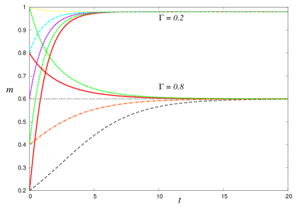
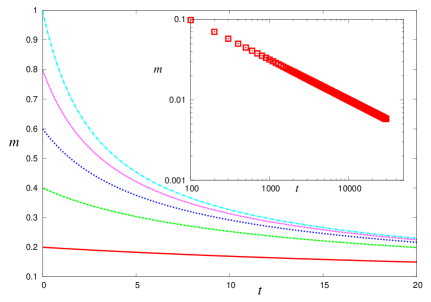
Figure 1: Typical behaviour of zero-temperature dynamics described by (13) with $\beta=\infty$ far from the critical point $\Gamma_{c}=J=1$ of quantum phase transition (left). The right panel denotes the zero-temperature dynamics at the critical point. The inset shows the log-log plot of $m(t)$ indicating that the dynamical exponent in the critical slowing down is $\nu^{{}^{\prime}}=1/2$.

In Figure 1(left), we plot the typical behaviour of zero-temperature dynamics (equation (13) with $\beta=\infty$) far from the critical point $\Gamma_{c}=J=1$ of quantum phase transition. We easily find that the dynamics exponentially converges to the steady state. The right panel denotes the zero-temperature dynamics at the critical point. The inset shows the log-log plot of $m(t)$ indicating that the dynamical exponent in the critical slowing down is $\nu^{{}^{\prime}}=1/2$. This fact is directly confirmed from equation (13) with $\beta=\infty$ near the critical point $dm/dt\simeq-(1-J\Gamma^{-1})m-(Jm)^{3}/2\Gamma^{3}+{\cal O}(m^{5})$, namely, $m(t)$ behaves around the critical point $\Gamma\simeq\Gamma_{c}=J$ as $m(t)=m(0)\,{\rm e}^{-t/(1-J\Gamma^{-1})^{-1}}$. At the critical point, the relaxation time diverges as $\tau_{\Gamma}\equiv(1-J\Gamma_{c}^{-1})^{-1}$ resulting in the critical slowing down as $m(t)\simeq{\rm e}^{-t/\tau_{\Gamma}}\to m(t)\simeq t^{-\nu^{{}^{\prime}}}$, $\nu^{{}^{\prime}}=1/2$. Of course, the exponent is the same as that of the ‘mean-field model’ universality class.

2.4 On the validity of static approximation

Without the static approximation, the following deterministic flow equations for each Trotter slice is obtained by substituting the form $P_{t}(m_{k})=\delta(m_{k}-m_{k}(t))$ and using the same way as deriving (13) as follows.

$$\frac{dm_{k}}{dt} = -m_{k}+\lim_{M\to\infty}\frac{{\rm tr}_{\{\sigma\}}\sigma(k)\exp[\frac{\beta J}{M}\sum_{l=1}^{M}m_{l}\sigma(l)+B\sum_{l=1}^{M}\sigma(l)\sigma(l+1)]}{{\rm tr}_{\{\sigma\}}\exp[\frac{\beta J}{M}\sum_{l=1}^{M}m_{l}\sigma(l)+B\sum_{l=1}^{M}\sigma(l)\sigma(l+1)]}$$ (14)

Obviously, the equation (14) is symmetric for the choice of $k$ as long as we use the periodic boundary condition $\mbox{\boldmath$\sigma$}_{1}=\mbox{\boldmath$\sigma$}_{M+1}$. This might be a justification to assume that the static approximation is correct at least for the present pure Ising system.

To confirm this argument, we carry out computer simulation for finite size system having $N=400$ spins. We observe the time evolving process of the histogram $P(m_{k})$ which is calculated from the $M=N=400$ copies of the Trotter slices. We show the result in Figure 2. In this simulation, we chose the initial configuration in each Trotter slice randomly (we set each spin variable $\sigma_{i}(k)$ to $+1$ with a fixed probability $p$) and choose the inverse temperature $\beta=2$ for $\Gamma=0.5$ and $\Gamma=0.6$. The time unit (the duration) of the update of $P(m_{k})$ is chosen as $1$ Monte Carlo step (MCS). From both panels in Figure 2, we find that at the beginning, the $P(m_{k})$ is distributed due to the random set-up of the initial configuration, however, the fluctuation rapidly (eventually) shrinks leading up to the delta function around ${\rm MCS}\sim 100$. After that, the $P(m_{k})$ evolves as a delta function with the peak located at the value of spontaneous magnetization which is explicitly indicated in the inset of each panel. It should be noted that we evaluated the value of order parameter at the time point in the Runge-Kutta method. Thus, the duration between the points to be evaluated is not the MCS but the Runge-Kutta step. Of course, some statistical errors for the finite system should be taken into account, however, the limited result here seems to support the validity of the static approximation even in the dynamical process.

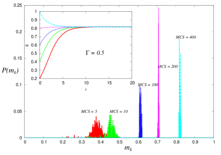
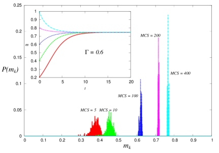
Figure 2: Time evolution of the distribution $P(m_{k})$ calculated for finite size system with $N=M=400$. We choose the inverse temperature $\beta=2$ for $\Gamma=0.5$ (left) and $\Gamma=0.6$ (right). The inset in each panel denotes the deterministic flows of spontaneous magnetization calculated by (13) for corresponding parameter sets.

3 Disordered systems: An application for Statistical-Mechanical Informatics

It is easy for us to extend the above formulation to some class of disordered spin systems, that is to say, the infinite-range random field Ising model which is often used to check the performance of image restoration analytically [26, 28, 29] as a bench mark test.

Here we consider a given original image $\mbox{\boldmath$\xi$}\equiv(\xi_{1},\cdots,\xi_{N})$ which is generated from the infinite-range ferromagnetic Ising model whose Gibbs measure (distribution for effective single spin) is described by $P(\xi_{i})={\rm e}^{\beta_{s}m_{0}\xi_{i}}/\{2\cosh(\beta_{s}m_{0})\}$, where $m_{0}$ denotes spontaneous magnetization at temperature $\beta_{s}^{-1}$. A snapshot $\xi$ from the distribution is degraded by additive white Gaussian noise (AWGN) with mean $a_{0}\xi_{i}$ and variance $a^{2}$, namely, each pixel in the degraded image $\mbox{\boldmath$\tau$}=(\tau_{1},\cdots,\tau_{N})$ is obtained by $\tau_{i}=a_{0}\xi_{i}+ax_{i}$ with $x_{i}\sim{\cal N}(0,1)$. From the Bayesian inference view point, we assume that the posterior $P(\mbox{\boldmath$\sigma$}|\mbox{\boldmath$\tau$})$ (here we define $\sigma$ as an estimate of the original image $\xi$) might be proportional to the logarithm of the effective Hamiltonian (2) with $J_{ij}=J\,\,\forall(i,j)$ and $h\neq 0$. The first and the second terms appearing in the right hand side of (2) correspond to the prior distribution and the likelihood function, respectively. Whereas, the third term is introduced to utilize quantum fluctuation to construct the Bayes estimate for each pixel (‘majority-vote decision’ on each pixel), namely, ${\rm sgn}(\langle\sigma_{i}^{z}\rangle)$.

In this section, we attempt to describe the recovering process of original image through the deterministic flows of several relevant order-parameters and image restoration measure, namely, the overlap function ${\cal M}\equiv N^{-1}\sum_{i}\xi_{i}\,{\rm sgn}(\langle\sigma_{i}^{z}\rangle)$.

For the above set-up of the problem, the local field on the site $i$ in the $k$-th Trotter slice now leads to

$$\phi_{i}(\mbox{\boldmath$\sigma$}_{k}:\sigma_{i}(k+1),\mbox{\boldmath$\tau$}) = \frac{J}{NM}\sum_{j}\sigma_{j}(k)+\frac{h}{M}\tau_{i}\sigma_{i}(k)+B\sigma_{i}(k+1).$$

As relevant order parameters, we choose $\mu_{k}=N^{-1}\sum_{i}\tau_{i}\sigma_{i}(k)$ and magnetization $m_{k}$. Then, we derive the differential equation with respect to $P_{t}(m_{k},\mu_{k})=\sum_{\mbox{\boldmath$\sigma$}_{k}}p_{t}(\mbox{\boldmath$\sigma$}_{k})\delta(m_{k}-m_{k}(\mbox{\boldmath$\sigma$}_{k}))\delta(\mu_{k}-\mu_{k}(\mbox{\boldmath$\sigma$}_{k}))$ as follows.

$$\frac{dP_{t}(m_{k},\mu_{k})}{dt} = \frac{\partial}{\partial m_{k}}\{m_{k}P_{t}(m_{k},\mu_{k})\}+\frac{\partial}{\partial\mu_{k}}\{\mu_{k}P_{t}(m_{k},\mu_{k})\}$$ (15)

$$- \frac{\partial}{\partial m_{k}}\left\{P_{t}(m_{k},\mu_{k})\frac{1}{N}\sum_{i}\tanh[\beta\phi_{i}(\mbox{\boldmath$\sigma$}_{k}:\sigma_{i}(k+1),\mbox{\boldmath$\tau$})]\right\}$$

$$- \frac{\partial}{\partial\mu_{k}}\left\{P_{t}(m_{k},\mu_{k})\frac{1}{N}\sum_{i}\tau_{i}\tanh[\beta\phi_{i}(\mbox{\boldmath$\sigma$}_{k}:\sigma_{i}(k+1),\mbox{\boldmath$\tau$})]\right\}$$

By assuming the self-averaging properties on the following physical quantities over both all possible paths in the imaginary-time axis and input data; original images and degrading processes (a particular realization of the quantity is identical to the average value and its deviation from the average eventually vanishes in the limit $N\to\infty$), we have

$$N^{-1}\sum_{i}\tanh[\beta\phi_{i}(\mbox{\boldmath$\sigma$}_{k}:\sigma_{i}(k+1),\mbox{\boldmath$\tau$})] = [\langle\sigma(k)\rangle_{*path}]_{data}$$

$$N^{-1}\sum_{i}\tau_{i}\tanh[\beta\phi_{i}(\mbox{\boldmath$\sigma$}_{k}:\sigma_{i}(k+1),\mbox{\boldmath$\tau$})] = [\tau\langle\sigma(k)\rangle_{*path}]_{data}$$

where we defined the two different kinds of the averages by

$$\langle\cdots\rangle_{*path} \equiv \lim_{M\to\infty}\frac{{\rm tr}_{\{\sigma\}}(\cdots)\exp[\frac{\beta}{M}\sum_{l=1}^{M}(Jm_{l}+h\tau)\sigma(l)+B\sum_{l=1}^{M}\sigma(l)\sigma(l+1)]}{{\rm tr}_{\{\sigma\}}\exp[\frac{\beta}{M}\sum_{l=1}^{M}(Jm_{l}+h\tau)\sigma(l)+B\sum_{l=1}^{M}\sigma(l)\sigma(l+1)]}$$

$$\mbox{}[\cdots]_{data} \equiv \frac{\sum_{\xi}{\rm e}^{\beta_{s}m_{0}\xi}}{2\cosh(\beta_{s}m_{0})}\int_{-\infty}^{\infty}(\cdots)\,{\exp}\left[-\frac{(\tau-a_{0}\xi)^{2}}{2a^{2}}\right]d\tau.$$ (16)

Under the static approximation, we obtain

$$\frac{dP_{t}(m,\mu)}{dt}=\frac{\partial}{\partial m}\{mP_{t}(m,\mu)\}+\frac{\partial}{\partial\mu}\{\mu P_{t}(m,\mu)\}$$

$$- \frac{\partial}{\partial m}\left\{P_{t}(m,\mu)\frac{\sum_{\xi}{\rm e}^{\beta_{s}m_{0}\xi}}{2\cosh(\beta_{s}m_{0})}\int_{-\infty}^{\infty}Dx\frac{\varXi_{m}^{(a,a_{0})}(\xi,x)\tanh\beta\sqrt{\{\varXi_{m}^{(a,a_{0})}(\xi,x)\}^{2}+\Gamma^{2}}}{\sqrt{\{\varXi_{m}^{(a,a_{0})}(\xi,x)\}^{2}+\Gamma^{2}}}\right\}$$

$$- \frac{\partial}{\partial\mu}\left\{P_{t}(m,\mu)\frac{\sum_{\xi}{\rm e}^{\beta_{s}m_{0}\xi}}{2\cosh(\beta_{s}m_{0})}\int_{-\infty}^{\infty}Dx\frac{(a_{0}\xi+ax)\varXi_{m}^{(a,a_{0})}(\xi,x)\tanh\beta\sqrt{\{\varXi_{m}^{(a,a_{0})}(\xi,x)\}^{2}+\Gamma^{2}}}{\sqrt{\{\varXi_{m}^{(a,a_{0})}(\xi,x)\}^{2}+\Gamma^{2}}}\right\}$$

with $\varXi_{m}^{(a,a_{0})}(\xi,x)\equiv Jm+ha_{0}\xi+hax$ and $Dx\equiv dx\,{\rm e}^{-x^{2}/2}/\sqrt{2\pi}$. Using the same way as the pure Ising system discussed in the previous section, we finally obtain the deterministic flow equations of the order-parameters $m$ and $\mu$ as follows.

$$\frac{dm}{dt} = -m+\frac{\sum_{\xi}{\rm e}^{\beta_{s}m_{0}\xi}}{2\cosh(\beta_{s}m_{0})}\int_{-\infty}^{\infty}Dx\frac{\varXi_{m}^{(a,a_{0})}(\xi,x)\tanh\beta\sqrt{\{\varXi_{m}^{(a,a_{0})}(\xi,x)\}^{2}+\Gamma^{2}}}{\sqrt{\{\varXi_{m}^{(a,a_{0})}(\xi,x)\}^{2}+\Gamma^{2}}}$$ (17)

$$\frac{d\mu}{dt} = -\mu+\frac{\sum_{\xi}{\rm e}^{\beta_{s}m_{0}\xi}}{2\cosh(\beta_{s}m_{0})}\int_{-\infty}^{\infty}Dx\frac{(a_{0}\xi+ax)\varXi_{m}^{(a,a_{0})}(\xi,x)\tanh\beta\sqrt{\{\varXi_{m}^{(a,a_{0})}(\xi,x)\}^{2}+\Gamma^{2}}}{\sqrt{\{\varXi_{m}^{(a,a_{0})}(\xi,x)\}^{2}+\Gamma^{2}}}.$$ (18)

For the solution of the above deterministic flows $(m,\mu)$ at time $t$, the overlap between the original image and degraded image is measured by

$${\cal M}(m,\mu) = \frac{\sum_{\xi}{\rm e}^{\beta_{s}m_{0}\xi}}{2\cosh(\beta_{s}m_{0})}\int_{-\infty}^{\infty}Dx\,{\rm sgn}[\hat{m}+(a_{0}\xi+ax)\hat{\mu}]$$ (19)

where $(\hat{m},\hat{\mu})$ is a solution of the following coupled equations

$$m = \frac{\sum_{\xi}{\rm e}^{\beta_{s}m_{0}\xi}}{2\cosh(\beta_{s}m_{0})}\int_{-\infty}^{\infty}Dx\,\tanh[\hat{m}+(a_{0}\xi+ax)\hat{\mu}]$$ (20)

$$\mu = \frac{\sum_{\xi}{\rm e}^{\beta_{s}m_{0}\xi}}{2\cosh(\beta_{s}m_{0})}\int_{-\infty}^{\infty}Dx\,[\hat{m}+(a_{0}\xi+ax)\hat{\mu}]\,\tanh[\hat{m}+(a_{0}\xi+ax)\hat{\mu}]$$ (21)

for a given point on the trajectory $(m,\mu)$ at time $t$. To obtain the overlap function (19) and (20)(21), we used the concept of dynamical replica theory (the DRT) [21, 22], namely, ‘equipartitioning’ and ‘self-averaging’ of the ${\cal M}$ during the evolution in time. As the derivation is a bit complicated, we shall show the detail in A.

We solve the equations (17)(18) with (19)-(21) numerically and show the results in Figure 3. We choose the set of the parameters for the original image as $\beta_{s}^{-1}=0.9$ ($m_{0}=0.523$) and $a_{0}=a=1$ which means that the corresponding optimal hyper-parameters are $h=a_{0}/a^{2}=1$ and $J^{-1}=\beta^{-1}$. We consider the zero-temperature restoration dynamics in which the fluctuation to make the Bayesian estimate is only quantum-mechanical one (it is controlled by the amplitude of quantum-mechanical tunneling $\Gamma$). In the left panel, the deterministic trajectories in the space $(m,\mu)$ are plotted for $\Gamma=0.6$. The state of system in which the image restoration is successfully achieved is in ferromagnetic phase. Thus, order-parameters $m$ and $\mu$ converge to the fixed point exponentially (there is no critical slowing down in this model system). In the right panel, we show the time evolution of the image restoration measure ${\cal M}$ for several values of $\Gamma$. From this panel, we find that some ‘non-monotonic’ behaviour is observed at the initial stage of the dynamics when we fail to set the amplitude to its optimal value ($\Gamma\sim 0.6$). Similar behaviour was reported in the Bayesian image restoration via thermal (classical) fluctuation [38].

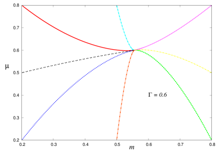
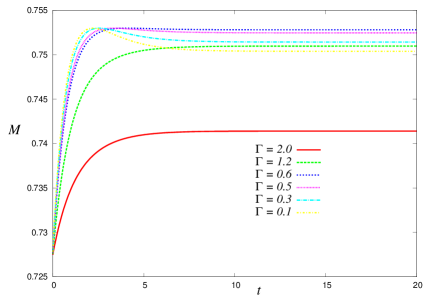
Figure 3: Trajectories in the phase space $(m,\mu)$ are plotted for $\Gamma=0.6$ (left). The parameters are chosen as $\beta_{s}^{-1}=0.9$ ($m_{0}=0.523$), $a_{0}=a=1$ and the corresponding hyper-parameters as $h=a_{0}/a^{2}=1$ and $J^{-1}=\beta^{-1}$. The right panel shows the evolution of image restoration measure, overlap function ${\cal M}$ in time for several values of the amplitude of quantum-mechanical tunneling $\Gamma$.

In the Bayesian framework, it is desired for us to obtain the estimate of each pixel and hyper-parameters simultaneously. In such case, we use the so-called EM algorithm based on the maximization of marginal likelihood criteria [39]. The quantum-mechanical extension and the formulation presented here is applicable to the simultaneous estimation for both micro and macro parameters.

4 Concluding remarks

In this paper, for a simplest quantum spin systems, we showed a formulation to describe the macroscopically deterministic flows of order parameters from the master equation whose transition probability is given by the Glauber-type. Under the static approximation, differential equations with respect to macroscopic order parameters were explicitly obtained from the master equation describing the microscopic-law. In the steady state, we found that the equations are identical to the saddle point equations for the equilibrium state of the same system. We also checked the validity of the static approximation by computer simulations and found that the result supports the validity of the approximation. Several possible extensions of our approach to disordered spin systems for statistical-mechanical informatics was discussed. Especially, we used our procedure to evaluate the decoding process of Bayesian image restoration. With the assistance of the concept of dynamical replica theory (the DRT), we derived the zero-temperature flow equation of image restoration measure showing some ‘non-monotonic’ behaviour in its time evolution. Of course, by using the present approach, one can evaluate the ‘inhomogeneous’ Markovian stochastic process of quantum Monte Carlo method (in which amplitude $\Gamma$ is time-dependent) such as quantum annealing. In the next step of the present study, we are planning to extend this formulation to the probabilistic information processing described by spin glasses such as quantum Hopfield model [40, 41] including a peculiar type of antiferromagnet [42].

Appendix A Derivation of overlap function: A dynamical approach

In this appendix, we show the derivation of overlap function for image restoration problem (19)-(21) by using a useful concept of dynamical replica theory (the DRT) [21, 22].

The problem here comes from the fact that the quantity ${\cal M}=N^{-1}\sum_{i}[\xi_{i}\,{\rm sgn}(\langle\sigma_{i}(k)\rangle_{path})]_{data}$ containing a single site expectation $\langle\sigma_{i}(k)\rangle_{path}$ is not observable in computer simulations of a single system. Therefore, we must introduce infinite number of ‘virtual copies’ (‘real replicas’ or ‘ensembles’ ) to evaluate the overlap function by using the law of large number. Namely, we evaluate the ‘real-time’ dependence of the overlap function as follows.

$${\cal M}(t) \equiv \lim_{L,N\to\infty}\frac{1}{N}\sum_{i}\xi_{i}\,{\rm sgn}\left(\frac{1}{L}\sum_{\rho=1}^{L}\sigma_{it}^{\rho}(k)\right)=\left[\left\langle\xi\,{\rm sgn}\left(\frac{1}{L}\sum_{\rho=1}^{L}\sigma_{1t}^{\rho}(k)\right)\right\rangle_{copy}\right]_{data}$$

$$= {\cal M}(m_{k}(t),\mu_{k}(t))$$

where $\rho=1,\cdots,L$ denote the copies of the original system in which $p_{t}(\mbox{\boldmath$\sigma$}^{\rho}(k))$ is the same. From the law of large number, we can expect $\lim_{L\to\infty}L^{-1}\sum_{\rho=1}^{L}\sigma_{it}^{l}(k)=\langle\sigma_{i}(k)\rangle_{copy}$. To calculate the expectation $\langle\cdots\rangle_{copy}$, we assume the equipartitioning in the $(m_{k},\mu_{k})$-subsells. Namely, explicit time-dependence of the expectation through $p_{t}(\mbox{\boldmath$\sigma$}^{\rho}(k))$ is now removed within the subsells as

$$\langle\cdots\rangle_{copy} = \frac{\sum_{\{\mbox{\boldmath$\sigma$}^{\rho}(k)\}}\prod_{\rho=1}^{L}p_{t}(\mbox{\boldmath$\sigma$}^{\rho}(k))(\cdots)\delta(m_{k}-m_{k}(\mbox{\boldmath$\sigma$}^{\rho}(k)))\delta(\mu_{k}-\mu_{k}(\mbox{\boldmath$\sigma$}^{\rho}(k)))}{\sum_{\{\mbox{\boldmath$\sigma$}^{\rho}(k)\}}\prod_{\rho=1}^{L}p_{t}(\mbox{\boldmath$\sigma$}^{\rho}(k))\delta(m_{k}-m_{k}(\mbox{\boldmath$\sigma$}^{\rho}(k)))\delta(\mu_{k}-\mu_{k}(\mbox{\boldmath$\sigma$}^{\rho}(k)))}$$

$$= \frac{\sum_{\{\mbox{\boldmath$\sigma$}^{\rho}(k)\}}\prod_{\rho=1}^{L}(\cdots)\delta(m_{k}-m_{k}(\mbox{\boldmath$\sigma$}^{\rho}(k)))\delta(\mu_{k}-\mu_{k}(\mbox{\boldmath$\sigma$}^{\rho}(k)))}{\sum_{\{\mbox{\boldmath$\sigma$}^{\rho}(k)\}}\prod_{\rho=1}^{L}\delta(m_{k}-m_{k}(\mbox{\boldmath$\sigma$}^{\rho}(k)))\delta(\mu_{k}-\mu_{k}(\mbox{\boldmath$\sigma$}^{\rho}(k)))}.$$

Then, assuming the self-averaging on the ${\cal M}$, we have ${\cal M}_{L}(m_{k},\mu_{k})$ in the limit of $N\to\infty$ as

$${\cal M}_{L}(m_{k},\mu_{k})$$

$$= \lim_{N\to\infty}\left[\frac{\sum_{\mbox{\boldmath$\sigma$}^{1}(k),\cdots,\mbox{\boldmath$\sigma$}^{L}(k)}\prod_{\rho=1}^{L}\delta(m_{k}-m_{k}(\mbox{\boldmath$\sigma$}^{\rho}(k)))\delta(\mu_{k}-\mu_{k}(\mbox{\boldmath$\sigma$}^{\rho}(k)))\xi_{1}{\rm sgn}\left(\frac{1}{L}\sum_{\rho=1}^{L}\sigma_{1}^{\rho}(k)\right)}{\sum_{\mbox{\boldmath$\sigma$}^{1}(k),\cdots,\mbox{\boldmath$\sigma$}^{L}(k)}\prod_{\rho=1}^{L}\delta(m_{k}-m_{k}(\mbox{\boldmath$\sigma$}^{\rho}(k)))\delta(\mu_{k}-\mu_{k}(\mbox{\boldmath$\sigma$}^{\rho}(k)))}\right]_{data}$$

$$= \lim_{n\to 0}\lim_{N\to\infty}\left[\sum_{\{\mbox{\boldmath$\sigma$}^{\rho\alpha}(k)\}}\xi_{1}\,{\rm sgn}\left(\frac{1}{L}\sum_{\rho=1}^{L}\sigma_{1}^{\rho 1}(k)\right)\prod_{\alpha=1}^{n}\prod_{\rho=1}^{L}\delta(m_{k}-m_{k}(\mbox{\boldmath$\sigma$}^{\rho\alpha}(k)))\delta(\mu_{k}-\mu_{k}(\mbox{\boldmath$\sigma$}^{\rho\alpha}(k)))\right]_{data}$$

where we used the fact

$$\left[\frac{{\rm tr}_{\{s\}}{\cal P}\psi}{{\rm tr}_{\{s\}}{\cal P}}\right]_{data} = \lim_{n\to 0}\left[\frac{({\rm tr}_{\{s\}}{\cal P}\psi)({\rm tr}_{\{s\}}{\cal P})^{n}}{{\rm tr}_{\{s\}}{\cal P}}\right]_{data}=\lim_{n\to 0}\left[{\rm tr}_{\{s^{\alpha}\}}\psi(s^{1})\prod_{\alpha=1}^{n}{\cal P}(\{s^{\alpha}\})\right]_{data}.$$

and introduced the replica index $\alpha=1,\cdots,n$ to carry out the average $[\cdots]_{data}$ by standard replica trick. It should be noted that $\mbox{\boldmath$\sigma$}\equiv(\sigma_{1}(k),\cdots,\sigma_{N}(k))$ and $\{\cdots\}$ denotes the set of spin variables for all possible combinations of copies and replicas $(\rho,\alpha)$. By using the integral representation for the delta-function, we obtain

$${\cal M}_{L}(m_{k},\mu_{k}) = \lim_{n\to 0}\lim_{N\to\infty}\int_{-\infty}^{\infty}\prod_{\rho\alpha}\frac{d\hat{m}_{k}^{\rho\alpha}d\hat{\mu}_{k}^{\rho\alpha}}{2\pi N}\,{\rm e}^{-iN\sum_{\rho\alpha}(m_{k}\hat{m}_{k}^{\rho\alpha}+\mu_{k}\hat{\mu}_{k}^{\rho\alpha})}$$

$$\times \sum_{\{\mbox{\boldmath$\sigma$}^{\rho\alpha}(k)\}}\xi_{1}\,{\rm sgn}\left(\frac{1}{L}\sum_{\rho=1}^{L}\sigma_{1}^{\rho 1}(k)\right){\rm e}^{-i\sum_{\rho\alpha}\hat{m}_{k}^{\rho\alpha}\sum_{i}\sigma_{i}^{\rho\alpha}(k)}\left[{\rm e}^{-i\sum_{\rho\alpha}\hat{\mu}_{k}^{\rho\alpha}\sum_{i}\tau_{i}\sigma_{i}^{\rho\alpha}(k)}\right]_{data}.$$

Now, under the static approximation, the quantum fluctuation appears through the quantities $m_{k}=m$ and $\mu_{k}=\mu$ which obeys (17)(18) at any time $t$. Therefore, from now on, we cancel the $k$-dependence. By simple transformation of the variables as $-i\hat{\mu}^{\rho\alpha}\mapsto\hat{\mu}^{\rho\alpha},-i\hat{m}^{\rho\alpha}\mapsto\hat{m}^{\rho\alpha}$ and carrying out the data average $[\cdots]_{data}$ over the effective single site distribution (16), one obtains

$${\cal M}_{L}(m,\mu) = \lim_{n\to 0}\lim_{N\to 0}\int_{-\infty}^{\infty}\prod_{\rho\alpha}\frac{d\hat{m}^{\rho\alpha}d\hat{\mu}^{\rho\alpha}}{2\pi N}\,{\rm e}^{-N\sum_{\rho\alpha}(m\hat{m}_{k}^{\rho\alpha}+\mu\hat{\mu}_{k}^{\rho\alpha})}$$ (22)

$$\times \left\{\frac{\sum_{\xi}{\rm e}^{\beta_{s}m_{0}\xi}}{2\cosh(\beta_{s}m_{0})}\int_{-\infty}^{\infty}\prod_{\rho\alpha}\left\{2\cosh[\hat{m}^{\rho\alpha}+(a_{0}\xi+ax)\hat{\mu}^{\rho\alpha}]\right\}\right\}^{N}$$

$$\times \frac{\sum_{\sigma^{\rho\alpha}}\xi_{1}{\rm sgn}\left(\frac{1}{L}\sum_{\rho=1}^{L}\sigma_{1}^{\rho 1}\right){\exp}[\sum_{\rho\alpha}\hat{m}^{\rho\alpha}\sigma^{\rho\alpha}+(a\xi+ax)\sum_{\rho\alpha}\hat{\mu}^{\rho\alpha}\sigma^{\rho\alpha}]}{\sum_{\sigma^{\rho\alpha}}{\exp}[\sum_{\rho\alpha}\hat{m}^{\rho\alpha}+(a\xi+ax)\sum_{\rho\alpha}\hat{\mu}^{\rho\alpha}\sigma^{\rho\alpha}]}$$

$$\times \lim_{n\to 0}\lim_{N\to 0}\int_{-\infty}^{\infty}d\mbox{\boldmath$\hat{m}$}d\mbox{\boldmath$\hat{\mu}$}\,{\exp}[N\Psi(\mbox{\boldmath$\hat{m}$},\mbox{\boldmath$\hat{\mu}$})]$$

$$\times \frac{\sum_{\sigma^{\rho\alpha}}\xi_{1}{\rm sgn}\left(\frac{1}{L}\sum_{\rho=1}^{L}\sigma_{1}^{\rho 1}\right){\exp}[\sum_{\rho\alpha}\hat{m}^{\rho\alpha}\sigma^{\rho\alpha}+(a\xi+ax)\sum_{\rho\alpha}\hat{\mu}^{\rho\alpha}\sigma^{\rho\alpha}]}{\sum_{\sigma^{\rho\alpha}}{\exp}[\sum_{\rho\alpha}\hat{m}^{\rho\alpha}+(a\xi+ax)\sum_{\rho\alpha}\hat{\mu}^{\rho\alpha}\sigma^{\rho\alpha}]}$$

with

$$\Psi(\mbox{\boldmath$\hat{m}$},\mbox{\boldmath$\hat{\mu}$}) \equiv -\sum_{\rho\alpha}(m\hat{m}^{\rho\alpha}+\mu\hat{\mu}^{\rho\alpha})+\log\left[\frac{\sum_{\xi}{\rm e}^{\beta_{s}m_{0}\xi}}{2\cosh(\beta_{s}m_{0})}\int_{-\infty}^{\infty}\prod_{\rho\alpha}\left\{2\cosh[\hat{m}^{\rho\alpha}+(a_{0}\xi+ax)\hat{\mu}^{\rho\alpha}]\right\}\right].$$

We should notice that in the above expression of the overlap function ${\cal M}_{L}(m,\mu)$, the condition $\xi_{1}={\rm sgn}(L^{-1}\sum_{\rho=1}^{L}\sigma_{\rho 1}(k))$ leading to ‘perfect image restoration’, namely, $\lim_{L\to\infty}{\cal M}_{L}=1$ immediately gives $\lim_{n\to 0}\lim_{N\to 0}\int_{-\infty}^{\infty}d\mbox{\boldmath$\hat{m}$}d\mbox{\boldmath$\hat{\mu}$}\,{\exp}[N\Psi(\mbox{\boldmath$\hat{m}$},\mbox{\boldmath$\hat{\mu}$})]=1$. Therefore, it is easy to find that the part $\lim_{n\to 0}\lim_{N\to 0}\int_{-\infty}^{\infty}d\mbox{\boldmath$\hat{m}$}d\mbox{\boldmath$\hat{\mu}$}\,{\exp}[N\Psi(\mbox{\boldmath$\hat{m}$},\mbox{\boldmath$\hat{\mu}$})]$ appearing in (22) is a normalization factor. Thus, the overlap function derived by the above dynamical approach now leads to

$${\cal M}_{L}(m,\mu) = \frac{\sum_{\sigma^{\rho\alpha}}\xi_{1}\,{\rm sgn}\left(\frac{1}{L}\sum_{\rho=1}^{L}\sigma_{1}^{\rho 1}\right){\exp}[\sum_{\rho\alpha}\hat{m}^{\rho\alpha}\sigma^{\rho\alpha}+(a\xi+ax)\sum_{\rho\alpha}\hat{\mu}^{\rho\alpha}\sigma^{\rho\alpha}]}{\sum_{\sigma^{\rho\alpha}}{\exp}[\sum_{\rho\alpha}\hat{m}^{\rho\alpha}\sigma^{\rho\alpha}+(a\xi+ax)\sum_{\rho\alpha}\hat{\mu}^{\rho\alpha}\sigma^{\rho\alpha}]}$$

where $\hat{m}$ or $\hat{\mu}$ should be chosen as a saddle point of the function $\Psi(\mbox{\boldmath$\hat{m}$},\mbox{\boldmath$\hat{\mu}$})$. Assuming the replica symmetric and the copy symmetric solution $\hat{m}^{\rho\alpha}=\hat{m},\hat{\mu}^{\rho\alpha}=\hat{\mu}\,\,\forall(\rho,\alpha)$, we obtain the function to be optimized at the saddle point.

$$\Psi_{RS}=\lim_{n\to 0}\lim_{N,L\to\infty}\frac{\Psi(\mbox{\boldmath$\hat{m}$},\mbox{\boldmath$\hat{\mu}$})}{nL}=-m\hat{m}-\mu\hat{\mu}+\frac{\sum_{\xi}{\rm e}^{\beta_{s}m_{0}\xi}}{2\cosh(\beta_{s}m_{0})}\int_{-\infty}^{\infty}Dx\cosh[\hat{m}+(a_{0}\xi+ax)\hat{\mu}]$$

Obviously we find that the saddle point is obtained by the equations (20) and (21). Then, the overlap function is evaluated as

$${\cal M}_{L}(m,\mu) = \frac{\sum_{\xi}\xi\,{\rm e}^{\beta_{s}m_{0}\xi}}{2\cosh(\beta_{s}m_{0})}\int_{-\infty}^{\infty}Dx\sum_{\sigma^{1},\cdots,\sigma^{L}}{\rm sgn}\left(\frac{1}{L}\sum_{\rho=1}^{L}\sigma_{1}^{\rho 1}\right)\prod_{\rho=1}^{L}\frac{{\rm e}^{\{\hat{m}+(a_{0}\xi+ax)\hat{\mu}\}\sigma_{1}^{\rho 1}}}{2\cosh[\hat{m}+(a_{0}\xi+ax)\hat{\mu}]}$$

$$= \int_{-\infty}^{\infty}dz\,\frac{\sum_{\xi}\xi\,{\rm e}^{\beta_{s}m_{0}\xi}}{2\cosh(\beta_{s}m_{0})}\int_{-\infty}^{\infty}Dx\sum_{\sigma^{1},\cdots,\sigma^{L}}{\rm sgn}(z)\delta\left(z-\frac{1}{L}\sum_{\rho=1}^{L}\sigma_{1}^{\rho 1}\right)$$

$$\times \prod_{\rho=1}^{L}\frac{{\rm e}^{\hat{m}+(a_{0}\xi+ax)\hat{\mu}}}{2\cosh[\hat{m}+(a_{0}\xi+ax)\hat{\mu}]}\equiv\int_{-\infty}^{\infty}dz\,{\rm sgn}(z){\cal P}_{L}(z)$$

with

$${\cal P}_{L}(z) \equiv \frac{\sum_{\xi}\xi\,{\rm e}^{\beta_{s}m_{0}\xi}}{2\cosh(\beta_{s}m_{0})}\int_{-\infty}^{\infty}Dx\sum_{\sigma^{1},\cdots,\sigma^{L}}\int_{-\infty}^{\infty}\frac{dy}{2\pi}\,{\rm e}^{iy(z-L^{-1}\sum_{\rho=1}^{L}\sigma_{1}^{\rho})}\prod_{\rho=1}^{L}\frac{{\rm e}^{\{\hat{m}+(a_{0}\xi+ax)\hat{\mu}\}\sigma_{1}^{\rho 1}}}{2\cosh[\hat{m}+(a_{0}\xi+ax)\hat{\mu}]}$$

$$= \int_{-\infty}^{\infty}\frac{dy}{2\pi}{\rm e}^{iyz}\frac{\sum_{\xi}\xi\,{\rm e}^{\beta_{s}m_{0}\xi}}{2\cosh(\beta_{s}m_{0})}\int_{-\infty}^{\infty}Dx\left\{\frac{\cosh[\hat{m}+(a_{0}\xi+ax)\hat{\mu}-iL^{-1}y]}{\cosh[\hat{m}+(a_{0}\xi+ax)\hat{\mu}]}\right\}^{L}$$

$$= \int_{-\infty}^{\infty}\frac{dy}{2\pi}{\rm e}^{iyz}\frac{\sum_{\xi}\xi\,{\rm e}^{\beta_{s}m_{0}\xi}}{2\cosh(\beta_{s}m_{0})}\int_{-\infty}^{\infty}Dx\left\{\cos(yL^{-1})-i\sin(yL^{-1})\tanh[\hat{m}+(a_{0}\xi+ax)\hat{\mu}]\right\}^{L}.$$

Thus, we have

$${\cal P}(z) \equiv \lim_{L\to\infty}{\cal P}_{L}(z)=\frac{\sum_{\xi}\xi\,{\rm e}^{\beta_{s}m_{0}\xi}}{2\cosh(\beta_{s}m_{0})}\int_{-\infty}^{\infty}Dx\int_{-\infty}^{\infty}\frac{dy}{2\pi}\,{\rm e}^{iy(z-\tanh[\hat{m}+(a_{0}\xi+ax)\hat{\mu}])}$$

$$= \frac{\sum_{\xi}\xi\,{\rm e}^{\beta_{s}m_{0}\xi}}{2\cosh(\beta_{s}m_{0})}\int_{-\infty}^{\infty}Dx\,\delta(z-\tanh[\hat{m}+(a_{0}\xi+ax)\hat{\mu}]).$$

Substituting the result into ${\cal M}_{L}$ and taking the limit of $L\to\infty$, we finally obtain

$${\cal M}(m,\mu) = \lim_{L\to\infty}{\cal M}_{L}(m,\mu)=\int_{-\infty}^{\infty}dz\,{\rm sgn}(z)\lim_{L\to\infty}{\cal P}_{L}(z)=\int_{-\infty}^{\infty}dz\,{\rm sgn}(z){\cal P}(z)$$

$$= \frac{\sum_{\xi}\xi\,{\rm e}^{\beta_{s}m_{0}\xi}}{2\cosh(\beta_{s}m_{0})}\int_{-\infty}^{\infty}Dx\,{\rm sgn}[\hat{m}+(a_{0}\xi+ax)\hat{\mu}]$$

where we used the fact ${\rm sgn}(\tanh(x))={\rm sgn}(x)$. This result is nothing but equation (19). As parameters $\hat{m}$ and $\hat{\mu}$ are related to the order-parameters $m$ and $\mu$ in equations (20)(21), overlap function ${\cal M}$ is influenced by quantum fluctuation through (20)(21) and the solution of equations (17)(18). The present study was financially supported by Grant-in-Aid Scientific Research on Priority Areas “Deepening and Expansion of Statistical Mechanical Informatics (DEX-SMI)” of The Ministry of Education, Culture, Sports, Science and Technology (MEXT) No. 18079001 and INSA (Indian National Science Academy) - JSPS (Japan Society of Promotion of Science) Bilateral Exchange Programme. The author thanks Saha Institute of Nuclear Physics for their warm hospitality during his stay in India.

References

References

- [1] Bishop C M 2006, Pattern Recognition and Machine Learning, (Singapore: Springer)
- [2] Opper M and Saad D 2001 Advanced Mean Field Methods: Theory and Practice (Massachusetts: The MIT Press)
- [3] Jordan M I 1998 Learning in Graphical Models (Massachusetts: The MIT Press)
- [4] Landau D P and Binder K 2000 A Guide to Monte Carlo Simulations in Statistical Physics (Cambridge: Cambridge University Press)
- [5] Mézard M, Parisi G and Virasoro M A 1987 Spin Glass Theory and Beyond (Singapore: World Scientific)
- [6] Binder K and Young A P 1986 Rev. Mod. Phys. 58 801
- [7] Young A P 1998 Spin Glass and Random Fields (Singapore: World Scientific)
- [8] Swendsen R H and Wang J S 1986 Phys. Rev. Lett. 57 2607, Swendsen R H and Wang J S 1987 Phys. Rev. Lett. 58 86
- [9] Hukushima K and Nemoto K 1996 J. Phys. Soc. Jpn. 65 1604
- [10] Kirkpatrick S, Gelatt Jr C D and Vecchi MP (1983) Science 220 671
- [11] Geman S and Geman D 1984 IEEE Trans. Pattern. Anal. and Mach. Intel. 11 721
- [12] Kadowaki T and Nishimori H 1998 Physical Review E 58 5355
- [13] Farhi E, Goldstone J, Gutmann S, Lapan J, Lundgren A and Preda P 2001 Science 292 472
- [14] Morita S and Nishimori H 2006 J. Phys. A 39 13903
- [15] Suzuki S and Okada M 2005 J. Phys. Soc. Jpn. 74 1649
- [16] Santoro G E and Tosatti 2006 J. Phys. A 41 209801
- [17] Suzuki M 1976 Prog. Theor. Phys. 56 1454
- [18] de Oriveira M J and Chiappin J R N 1997 Physica A 238 307
- [19] Coolen A C C and Ruijgrok Th W 1988 Phys. Rev. A 38 4253
- [20] Hopfield J J 1982 PNAS 79 2554
- [21] Coolen A C C and Sherrington D 1994 Phys. Rev. Let. 49 1921
- [22] Coolen A C C, Laughton S N and Sherrington D 1996 Phys. Rev. B 53 8184
- [23] Sherrington D and Kirkpatrick S 1975 Phys. Rev. Lett. 35 1792
- [24] Nishimori H 2001 Statistical Physics of Spin Glasses and Information Processing: An Introduction (Oxford: Oxford University Press)
- [25] Tanaka K and Horiguchi T 1997 IEICE J80-A-12 2217 (in Japanese)
- [26] Nishimori H and Wong K Y M 1999 Phys. Rev. E 60 132
- [27] Tanaka K 2002 J. Phys. A: Math. Gen. 35 R81
- [28] Inoue J 2001 Phys. Rev. E 63 046114
- [29] Inoue J 2005 Quantum Spin Glasses, Quantum Annealing, and Probabilistic Information Processing, in Quantum Annealing and Related Optimization Methods Lecture Notes in Physics 679, ed Das A and Chakrabarti B K (Berlin Heidelberg: Springer) p 259
- [30] Chakrabarti K, Dutta A and Sen P 1996 Quantum Ising Phases and Transitions in Transverse Ising Models (Heidelberg: Springer)
- [31] Sachdev S 1999 Quantum Phase Transitions (Cambridge: Cambridge University Press)
- [32] Sourlas N 1989 Nature 339 693
- [33] Inoue J, Saika Y and Okada M 2009 J. Phys: Conference Series 143 012019
- [34] Suzuki M 1966 J. Phys. Soc. Japan 21 2140
- [35] Elliot R J, Pfeuty P and Wood C 1970 Phys. Rev. lett. 25 443
- [36] Feynman R P and Hibbs A R 1965 Quantum Mechanics and Path Integrals (New York: McGraw-Hill)
- [37] Kleinert H 2009 Path Integrals in Quantum Mechanics, Statistics, Polymer Physics, and Financial Markets (Singapore: World Scientific)
- [38] Ozeki T and Okada M 2003 J. Phys. A 36 11011
- [39] Inoue J and Tanaka K 2002 Phys. Rev. E 65 016125
- [40] Ma Y Q and Gong C D 1992 Phys. Rev. B 45 793
- [41] Nishimori H and Nonomura Y 1996 J. Phys. Soc. Japan 65 3780
- [42] Chandra A K, Inoue J and Chakrabarti B K 2010 Phys. Rev. E (to appear)