The M-Wright function

in time-fractional diffusion processes:

a tutorial survey

Francesco MAINARDI^a, Antonio MURA^b, and Gianni PAGNINI^c

^a Department of Physics, University of Bologna, and INFN,

Via Irnerio 46, I-40126 Bologna, Italy;

E-mail: francesco.mainardi@unibo.it  ^b CRESME Ricerche S.p.A,

Viale Gorizia 25C, I-00199 Roma, Italy;

E-mail: anto.mura@gmail.com ^c CRS4, Centro Ricerche Studi Superiori e Sviluppo in Sardegna,

Polaris Bldg. 1, I-09010 Pula (Cagliari), Italy;

E-mail: pagnini@crs4.it

Abstract

In the present review we survey the properties of a transcendental function of the Wright type, nowadays known as $M$-Wright function, entering as a probability density in a relevant class of self-similar stochastic processes that we generally refer to as time-fractional diffusion processes. Indeed, the master equations governing these processes generalize the standard diffusion equation by means of time-integral operators interpreted as derivatives of fractional order. When these generalized diffusion processes are properly characterized with stationary increments, the $M$-Wright function is shown to play the same key role as the Gaussian density in the standard and fractional Brownian motions. Furthermore, these processes provide stochastic models suitable for describing phenomena of anomalous diffusion of both slow and fast type.

1 Introduction

By time-fractional diffusion processes we mean certain diffusion-like phenomena governed by master equations containing fractional derivatives in time whose fundamental solution can be interpreted as a probability density function ($pdf$) in space evolving in time. It is well known that for the most elementary diffusion process, the Brownian motion, the master equation is the standard linear diffusion equation whose fundamental solution is the Gaussian density with a spatial variance growing linearly in time. In such case we speak about normal diffusion, reserving the term anomalous diffusion when the variance grows differently. A number of stochastic models for explaining anomalous diffusion have been introduced in literature, among them we like to quote the fractional Brownian motion, see e.g. [50, 70], the Continuous Time Random Walk, see e.g. [25, 51, 53, 63], the Lévy flights, see e.g. [11], the Schneider grey Brownian motion, see [64, 65], and, more generally, random walk models based on evolution equations of single and distributed fractional order in time and/or space, see e.g. [7, 8, 9], [23, 24], [33, 34], [77, 78].

In this survey paper we focus our attention on modifications of the standard diffusion equation, where the time can be stretched by a power law ($t\to t^{\alpha}$, $0<\alpha<2$) and the first-order time derivative can be replaced by a derivative of non-integer order $\beta$ ($0<\beta\leq 1$). In these cases of generalized diffusion processes the corresponding fundamental solution still keeps the meaning of a spatial $pdf$ evolving in time and is expressed in terms of a special function of the Wright type that reduces to the Gaussian when $\beta=1$. This transcendental function, nowadays known as $M$-Wright function, will be shown to play a fundamental role for a general class of self-similar stochastic processes with stationary increments, which provide stochastic models for anomalous diffusion, as recently shown by Mura et al. [55, 56, 57, 58].

In Section 2 we provide the reader with the essential notions and notations concerning the integral transforms and fractional calculus, which are necessary in the rest of the paper. In Section 3 we introduce in the complex plane ${\rm C\hskip-4.8pt\vrule height=6.0pt,width=0.1831pt\hskip 5.0pt}$ the series and integral representations of the general Wright function denoted by $W_{\lambda,\mu}(z)$ and of the two related auxiliary functions $F_{\nu}(z)$, $M_{\nu}(z)$, which depend on a single parameter. In Section 4 we consider our auxiliary functions in real domain pointing out their main properties involving their integrals and their asymptotic representations. Mostly, we restrict our attention to the second auxiliary function, that we call $M$-Wright function, when its variable is in $\vbox{\hbox to8.9pt{I\hskip-2.1ptR\hfil}}\;^{+}$ or in all of IR   but extended in symmetric way. We derive a fundamental formula for the absolute moments of this function in $\vbox{\hbox to8.9pt{I\hskip-2.1ptR\hfil}}\;^{+}$, which allows us to obtain its Laplace and Fourier transforms. In Section 5 we consider some types of generalized diffusion equations containing time partial derivatives of fractional order and we express their fundamental solutions in terms of the $M$-Wright functions evolving in time with a given self-similarity law. In Section 6 we stress how the $M$-Wright function emerges as a natural generalization of the Gaussian probability density for a class of self-similar stochastic processes with stationary increments, depending on two parameters ($\alpha,\beta$). These processes are defined in a unique way by requiring the determination of any multi-point probability distribution and include the well-known standard and fractional Brownian motion. We refer to this class as the generalized grey Brownian motion ($ggBm$), because it generalizes the grey Brownian motion ($gBm$) introduced by Schneider [64, 65]. Finally, a short concluding discussion is drawn. In Appendix A we derive the fundamental solution of the time-fractional diffusion equation. In Appendix B we outline the relevance of the $M$-Wright function in time-fractional drift processes entering as subordinators in time-fractional diffusion.

2 Notions and Notations

Integral transforms pairs.

In our analysis we will make extensive use of integral transforms of Laplace, Fourier and Mellin type so we first introduce our notation for the corresponding transform pairs. We do not point out the conditions of validity and the main rules, since they are given in any textbook on advanced mathematics.

Let

$$\widetilde{f}(s)={\cal L}\left\{f(r);r\to s\right\}=\int_{0}^{\infty}{\rm e}^{\displaystyle\,-sr}\,f(r)\,dr\,,$$

be the Laplace transform of a sufficiently well-behaved function $f(r)$ with $r\in\vbox{\hbox to8.9pt{I\hskip-2.1ptR\hfil}}\;^{+}$, $s\in{\rm C\hskip-4.8pt\vrule height=6.0pt,width=0.1831pt\hskip 5.0pt}$, and let

$$f(r)={\cal L}^{-1}\left\{\widetilde{f}(s);s\to r\right\}=\frac{1}{2\pi i}\,\int_{Br}{\rm e}^{\displaystyle\,+sr}\,\widetilde{f}(s)\,ds\,,$$

be the inverse Laplace transform, where $Br$ denotes the so-called Bromwich path, a straight line parallel to the imaginary axis in the complex $s$-plane. Denoting by $\,\stackrel{{\scriptstyle{\cal L}}}{{\leftrightarrow}}\,$ the justaposition of the original function $f(r)$ with its Laplace transform $\widetilde{f}(s)$, the Laplace transform pair reads

$$f(r)\,\,\stackrel{{\scriptstyle{\cal L}}}{{\leftrightarrow}}\,\,\widetilde{f}(s)\,.$$

Let

$$\widehat{f}(\kappa)={\cal F}\left\{f(x);x\rightarrow\kappa\right\}=\int_{-\infty}^{+\infty}{\rm e}^{\displaystyle\,+i\kappa x}\,f(x)\,dx\,,$$

be the Fourier transform of a sufficiently well-behaved function $f(x)$ with $x\in\vbox{\hbox to8.9pt{I\hskip-2.1ptR\hfil}}\;$, $\kappa\in\vbox{\hbox to8.9pt{I\hskip-2.1ptR\hfil}}\;$, and let

$$f(x)={\cal F}^{-1}\left\{\widehat{f}(\kappa);\kappa\to x\right\}=\frac{1}{2\pi}\,\int_{-\infty}^{+\infty}{\rm e}^{\displaystyle\,-i\kappa x}\,\widehat{f}(\kappa)\,d\kappa\,,$$

be the inverse Fourier transform. Denoting by $\,\stackrel{{\scriptstyle{\cal F}}}{{\leftrightarrow}}\,$ the justaposition of the original function $f(x)$ with its Fourier transform $\widehat{f}(\kappa)$, the Fourier transform pair reads

$$f(x)\,\,\stackrel{{\scriptstyle{\cal F}}}{{\leftrightarrow}}\,\,\widehat{f}(\kappa)\,.$$

Let

$$f^{*}(s)={\cal M}\left\{f(r);r\to s\right\}=\int_{0}^{\infty}r^{\displaystyle\,s-1}\,f(r)\,dr\,,$$

be the Mellin transform of a sufficiently well-behaved function $f(r)$ with $r\in\vbox{\hbox to8.9pt{I\hskip-2.1ptR\hfil}}\;^{+}$, $s\in{\rm C\hskip-4.8pt\vrule height=6.0pt,width=0.1831pt\hskip 5.0pt}$, and let

$$f(r)={\cal M}^{-1}\left\{f^{*}(s);s\to r\right\}=\frac{1}{2\pi i}\,\int_{Br}r^{\displaystyle\,-s}\,f^{*}(s)\,ds\,,$$

be the inverse Mellin transform. Denoting by $\,\stackrel{{\scriptstyle{\cal M}}}{{\leftrightarrow}}\,$ the justaposition of the original function $f(r)$ with its Mellin transform $f^{*}(s)$, the Mellin transform pair reads

$$f(r)\,\,\stackrel{{\scriptstyle{\cal M}}}{{\leftrightarrow}}\,\,f^{*}(s)\,.$$

Essentials of fractional calculus with support in $\vbox{\hbox to8.9pt{I\hskip-2.1ptR\hfil}}\;^{+}\,$.

Fractional calculus is the branch of mathematical analysis that deals with pseudo-differential operators that extend the standard notions of integrals and derivatives to any positive non-integer order. The term fractional is kept only for historical reasons. Let us restrict our attention to sufficiently well-behaved functions $f(t)$ with support in $\vbox{\hbox to8.9pt{I\hskip-2.1ptR\hfil}}\;^{+}$. Two main approaches exist in the literature of fractional calculus to define the operator of derivative of non integer order for these functions, referred to Riemann-Liouville and to Caputo. Both approaches are related to the so-called Riemann-Liouville fractional integral defined for any order $\mu>0$ as

$$J_{t}^{\mu}f(t):=\frac{1}{\Gamma(\mu)}\int_{0}^{t}(t-\tau)^{\mu-1}f(\tau)\,d\tau\,.$$

We note the convention $J_{t}^{0}=I$ (Identity) and the semigroup property

$$J_{t}^{\mu}\,J_{t}^{\nu}=J_{t}^{\nu}\,J_{t}^{\mu}=J_{t}^{\mu+\nu}\,,\quad\mu\geq 0\,,\;\nu\geq 0\,.$$

The fractional derivative of order $\mu>0$ in the Riemann-Liouville sense is defined as the operator $\,D_{t}^{\mu}$ which is the left inverse of the Riemann-Liouville integral of order $\mu$ (in analogy with the ordinary derivative), that is

$$D_{t}^{\mu}\,J_{t}^{\mu}=I\,,\quad\mu>0\,.$$

If $m$ denotes the positive integer such that $m-1<\mu\leq m\,,$ we recognize from Eqs. (2.11) and (2.12): $\,D_{t}^{\mu}\,f(t):=\,D_{t}^{m}\,J_{t}^{m-\mu}\,f(t)\,,$ hence

$$D_{t}^{\mu}\,f(t)=\,\left\{\begin{array}[]{ll}{\displaystyle\frac{d^{m}}{dt^{m}}}\left[{\displaystyle\frac{1}{\Gamma(m-\mu)}\int_{0}^{t}\frac{f(\tau)\,d\tau}{(t-\tau)^{\mu+1-m}}}\right],&m-1<\mu<m,\\ {\displaystyle\frac{d^{m}}{dt^{m}}f(t)}\,,&\mu=m.\end{array}\right.$$

For completeness we define $D_{t}^{0}=I$.

On the other hand, the fractional derivative of order $\mu>0$ in the Caputo sense is defined as the operator $\,{}_{*}D_{t}^{\mu}$ such that ${}_{*}D_{t}^{\mu}\,f(t):=\,J_{t}^{m-\mu}\,D_{t}^{m}\,f(t)\,,$ hence

$${}_{*}D_{t}^{\mu}\,f(t)=\,\left\{\begin{array}[]{ll}{\displaystyle\frac{1}{\Gamma(m-\mu)}}\,{\displaystyle\int_{0}^{t}{\displaystyle\frac{f^{(m)}(\tau)\,d\tau}{(t-\tau)^{\mu+1-m}}}}\,,&m-1<\mu<m,\\ {\displaystyle\frac{d^{m}}{dt^{m}}f(t)}\,,&\mu=m.\end{array}\right.$$

We note the different behavior of the two derivatives in the limit $\mu\to(m-1)^{+}$. In fact,

$$\mu\to(m-1)^{+}\;\left\{\begin{array}[]{ll}&D_{t}^{\mu}f(t)\to D_{t}^{m}\,J_{t}^{1}\,f(t)=D_{t}^{(m-1)}\,f(t)\\ &{}_{*}D_{t}^{\mu}f(t)\to J_{t}^{1}\,D_{t}^{m}\,f(t)=D_{t}^{(m-1)}\,f(t)-D_{t}^{(m-1)}f(0^{+})\,,\end{array}\right.$$

where the limit for $t\to 0^{+}$ is taken after the operation of derivation.

Furthermore, recalling the Riemann-Liouville fractional integral and derivative of the power law for $t>0$,

$$\left\{\begin{array}[]{ll}&J_{t}^{\mu}\,t^{\gamma}={\displaystyle\frac{\Gamma(\gamma+1)}{\Gamma(\gamma+1+\mu)}\,t^{\gamma+\mu}\,,}\\ &D_{t}^{\mu}\,t^{\gamma}={\displaystyle\frac{\Gamma(\gamma+1)}{\Gamma(\gamma+1-\mu)}\,t^{\gamma-\mu}\,,}\end{array}\right.\quad\mu>0\,,\;\gamma>-1\,,$$

we find the relationship between the two types of fractional derivative,

$$D^{\mu}\left[f(t)-\sum_{k=0}^{m-1}\frac{t^{k}}{k!}\,f^{(k)}(0^{+})\right]=\,_{*}D_{t}^{\mu}\,f(t)\,.$$

We note that the Caputo definition for the fractional derivative incorporates the initial values of the function and of its integer derivatives of lower order. The subtraction of the Taylor polynomial of degree $m-1$ at $t=0^{+}$ from $f(t)$ is a sort of regularization of the fractional derivative. In particular, according to this definition, the relevant property that the derivative of a constant is zero is preserved for the fractional derivative.

Let us finally point out the rules for the Laplace transform with respect to the fractional integral and the two fractional derivatives. These rules are expected to properly generalize the well-known rules for standard integrals and derivatives.

For the Riemann-Liouville fractional integral we have

$${\cal L}\left\{J_{t}^{\mu}\,f(t);t\to s\right\}=\frac{\widetilde{f}(s)}{s^{\mu}}\,,\quad\mu\geq 0\,.$$

For the Caputo fractional derivative we consequently get

$${\cal L}\left\{{}_{*}D_{t}^{\mu}\,f(t);t\to s\right\}=s^{\mu}\,\widetilde{f}(s)-\sum_{k=0}^{m-1}s^{\mu-1-k}\,f^{(k)}(0^{+})\,,\;m-1<\mu\leq m\,,$$

where $f^{(k)}(0^{+}):={\displaystyle\lim_{t\to 0^{+}}}\,f^{(k)}(t)$. The corresponding rule for the Riemann-Liouville fractional derivative is more cumbersome and it reads

$${\cal L}\left\{D_{t}^{\mu}\,f(t);t\to s\right\}=s^{\mu}\,\widetilde{f}(s)-\sum_{k=0}^{m-1}\,\left[D_{t}^{k}\,J_{t}^{(m-\mu)}\right]\,f(0^{+})\,s^{m-1-k},\;m-1<\mu\leq m,$$

where the limit for $t\to 0^{+}$ is understood to be taken after the operations of fractional integration and derivation. As soon as all the limiting values $f^{(k)}(0^{+})$ are finite and $m-1<\mu<m$, formula (2.20) for the Riemann-Liouville derivative simplifies into

$${\cal L}\left\{D_{t}^{\mu}\,f(t);t\to s\right\}=s^{\mu}\,\widetilde{f}(s)\,,\quad m-1<\mu<m\,.$$

In the special case $f^{(k)}(0^{+})=0$ for $k=0,1,m-1$, we recover the identity between the two fractional derivatives. The Laplace transform rule (2.19) was practically the key result of Caputo [5, 6] in defining his generalized derivative in the late sixties. The two fractional derivatives have been well discussed in the 1997 survey paper by Gorenflo and Mainardi [21], see also [42], and in the 1999 book by Podlubny [59]. In these references the Authors have pointed out their preference for the Caputo derivative in physical applications where initial conditions are usually expressed in terms of finite derivatives of integer order.

For further reading on the theory and applications of fractional calculus we recommend the recent treatise by Kilbas et al. [29].

3 The functions of the Wright type

The general Wright function.

The Wright function, that we denote by $W_{\lambda,\mu,}(z)$, is so named in honour of E. Maitland Wright, the eminent British mathematician, who introduced and investigated this function in a series of notes starting from 1933 in the framework of the asymptotic theory of partitions, see [73, 74, 75]. The function is defined by the series representation, convergent in the whole $z$-complex plane,

$$W_{\lambda,\mu}(z):=\sum_{n=0}^{\infty}\frac{z^{n}}{n!\,\Gamma(\lambda n+\mu)}\,,\quad\lambda>-1\,,\;\mu\in{\rm C\hskip-4.8pt\vrule height=6.0pt,width=0.1831pt\hskip 5.0pt}\,.$$

Originally, Wright assumed $\lambda\geq 0$, and, only in 1940 [76], he considered $-1<\lambda<0$. We note that in Chapter 18 of Vol. 3 of the handbook of the Bateman Project [12], devoted to Miscellaneous Functions, presumably for a misprint, the parameter $\lambda$ of the Wright function is restricted to be non negative. When necessary, we propose to distinguish the Wright functions in two kinds according to $\lambda\geq 0$ (first kind) and $-1<\lambda<0$ (second kind).

For more details on Wright functions the reader can consult e.g. [19, 20, 28, 30, 39, 69, 71, 72] and references therein.

The integral representation of the Wright function reads

$$W_{\lambda,\mu}(z)=\frac{1}{2\pi i}\,\int_{Ha}\!\!{\rm e}^{\,\displaystyle\sigma+z\sigma^{-\lambda}}\,\frac{d\sigma}{\sigma^{\mu}}\,,\quad\lambda>-1\,,\;\mu\in{\rm C\hskip-4.8pt\vrule height=6.0pt,width=0.1831pt\hskip 5.0pt}\,,$$

where $Ha$ denotes the Hankel path. We remind that the Hankel path is a loop that starts from $-\infty$ along the lower side of the negative real axis, encircles the circular area around the origin with radius $\epsilon\to 0$ in the positive sense, and ends at $-\infty$ along the upper side of the negative real axis. The equivalence of the series and integral representations is easily proved using Hankel formula for the Gamma function

$$\frac{1}{\Gamma(\zeta)}=\int_{Ha}{\rm e}^{\,\displaystyle u}\,u^{-\zeta}\,du\,,\quad\zeta\in{\rm C\hskip-4.8pt\vrule height=6.0pt,width=0.1831pt\hskip 5.0pt}\,,$$

and performing a term-by-term integration. In fact,

$$W_{\lambda,\mu}(z)=\frac{1}{2\pi i}\,\int_{Ha}\!\!{\rm e}^{\,\displaystyle\sigma+z\sigma^{-\lambda}}\,\frac{d\sigma}{\sigma^{\mu}}=\frac{1}{2\pi i}\,\int_{Ha}\!\!{\rm e}^{\,\displaystyle\sigma}\,\left[\sum_{n=0}^{\infty}\frac{z^{n}}{n!}\,\sigma^{-\lambda n}\right]\,\frac{d\sigma}{\sigma^{\mu}}$$

$$=\sum_{n=0}^{\infty}\frac{z^{n}}{n!}\left[\frac{1}{2\pi i}\int_{Ha}\!\!{\rm e}^{\,\displaystyle\sigma}\,\sigma^{-\lambda n-\mu}\,d\sigma\right]=\sum_{n=0}^{\infty}\frac{z^{n}}{n!\,\Gamma[\lambda n+\mu]}\,.$$

It is possible to prove that the Wright function is entire of order $1/(1+\lambda)\,,$ hence it is of exponential type only if $\lambda\geq 0$ (which corresponds to Wright functions of the first kind). The case $\lambda=0$ is trivial since $W_{0,\mu}(z)={{\rm e}^{\,z}/\Gamma(\mu)}\,,$ provided that $\mu\neq 0,-1,-2,\dots$.

The auxiliary functions of the Wright type.

Mainardi, in his first analysis of the time-fractional diffusion equation [36, 48], aware of the Bateman handbook [12], but not yet of the 1940 paper by Wright [76], introduced the two (Wright-type) entire auxiliary functions,

$$F_{\nu}(z):=W_{-\nu,0}(-z)\,,\quad 0<\nu<1\,,$$

and

$$M_{\nu}(z):=W_{-\nu,1-\nu}(-z)\,,\quad 0<\nu<1\,,$$

inter-related through

$$F_{\nu}(z)=\nu\,z\,M_{\nu}(z)\,.$$

As a matter of fact, functions $F_{\nu}(z)$ and $M_{\nu}(z)$ are particular cases of the Wright function of the second kind $W_{\lambda,\mu}(z)$ by setting $\lambda=-\nu$ and $\mu=0$ or $\mu=1$, respectively.

Hereafter, we provide the series and integral representations of the two auxiliary functions derived from the general formulas (3.1) and (3.2), respectively.

The series representations for the auxiliary functions read

$$F_{\nu}(z):={\displaystyle\sum_{n=1}^{\infty}\frac{(-z)^{n}}{n!\,\Gamma(-\nu n)}}={\displaystyle\frac{1}{\pi}\,\sum_{n=1}^{\infty}\frac{(-z)^{n-1}}{n!}\,\Gamma(\nu n+1)\,\sin(\pi\nu n)\,,}$$

and

$$M_{\nu}(z):={\displaystyle\sum_{n=0}^{\infty}\frac{(-z)^{n}}{n!\,\Gamma[-\nu n+(1-\nu)]}}={\displaystyle\frac{1}{\pi}\,\sum_{n=1}^{\infty}\,\frac{(-z)^{n-1}}{(n-1)!}\,\Gamma(\nu n)\,\sin(\pi\nu n)}\,.$$

The second series representations in Eqs. (3.6)-(3.7) have been obtained by using the reflection formula for the Gamma function $\,\Gamma(\zeta)\,\Gamma(1-\zeta)=\pi/\sin\,\pi\zeta$.

As an exercise, the reader can directly prove that the radius of convergence of the power series in (3.6)-(3.7) is infinite for $0<\nu<1$ without being aware of Wright’s results, as it was shown independently by Mainardi [36], see also [59].

Furthermore, we have $F_{\nu}(0)=0$ and $M_{\nu}(0)=1/\Gamma(1-\nu)$. We note that relation (3.5) between the two auxiliary functions can be easily deduced from (3.6)-(3.7), by using the basic property of the Gamma function $\Gamma(\zeta+1)=\zeta\,\Gamma(\zeta)$.

The integral representations for the auxiliary functions read

$$F_{\nu}(z):=\frac{1}{2\pi i}\int_{Ha}\!\!{\rm e}^{\displaystyle\,\sigma-z\sigma^{\nu}}d\sigma\,,$$

$$M_{\nu}(z):=\frac{1}{2\pi i}\int_{Ha}\!\!{\rm e}^{\displaystyle\,\sigma-z\sigma^{\nu}}\frac{d\sigma}{\sigma^{1-\nu}}\,.$$

We note that relation (3.5) can be obtained also from (3.8)-(3.9) with an integration by parts. In fact,

$$\begin{array}[]{ll}M_{\nu}(z)&={\displaystyle\int_{Ha}\!\!{\rm e}^{\displaystyle\,\sigma-z\sigma^{\nu}}\,\frac{d\sigma}{\sigma^{1-\nu}}}={\displaystyle\int_{Ha}\!\!{\rm e}^{\displaystyle\,\sigma}\,\left(-\frac{1}{\nu z}\,\frac{d}{d\sigma}{\rm e}^{\displaystyle\,-z\sigma^{\nu}}\right)\,d\sigma}\\ \\ &={\displaystyle\frac{1}{\nu z}\,\int_{Ha}\!\!{\rm e}^{\displaystyle\,\sigma-z\sigma^{\nu}}\,d\sigma}={\displaystyle\frac{F_{\nu}(z)}{\nu z}}\,.\end{array}$$

The equivalence of the series and integral representations is easily proved by using the Hankel formula for the Gamma function and performing a term-by-term integration.

Special cases.

Explicit expressions of $F_{\nu}(z)$ and $M_{\nu}(z)$ in terms of known functions are expected for some particular values of $\nu$. Mainardi and Tomirotti [48] have shown that for $\nu=1/q\,,$ where $q\geq 2\,$ is a positive integer, the auxiliary functions can be expressed as a sum of simpler $(q-1)$ entire functions. In the particular cases $q=2$ and $q=3$ we find

$$\!\!M_{1/2}(z)\!=\!\frac{1}{\sqrt{\pi}}\,\sum_{m=0}^{\infty}(-1)^{m}\,{\left(\frac{1}{2}\right)}_{m}\,\frac{z^{2m}}{(2m)!}\!=\!\frac{1}{\sqrt{\pi}}\,{\rm exp}\,\left(-{\,z^{2}/4}\right),$$

and

$$\begin{array}[]{ll}M_{1/3}(z)&={\displaystyle\frac{1}{\Gamma(2/3)}\,\sum_{m=0}^{\infty}{\left(\frac{1}{3}\right)}_{m}\,\frac{z^{3m}}{(3m)!}-\,\frac{1}{\Gamma(1/3)}\,\sum_{m=0}^{\infty}{\left(\frac{2}{3}\right)}_{m}\,\frac{z^{3m+1}}{(3m+1)!}}\\ &={\displaystyle 3^{2/3}\,{\rm Ai}\left({z/3^{1/3}}\right)}\,,\end{array}$$

where $Ai$ denotes the Airy function.

Furthermore, it can be proved that $M_{1/q}(z)$ satisfies the differential equation of order $q-1$

$$\frac{d^{q-1}}{dz^{q-1}}\,M_{1/q}(z)+\frac{(-1)^{q}}{q}\,z\,M_{1/q}(z)=0\,,$$

subjected to the $q-1$ initial conditions at $z=0$, derived from (3.7),

$$M_{1/q}^{(h)}(0)=\frac{(-1)^{h}}{\Gamma[(1-(h+1)/q]}=\frac{(-1)^{h}}{{\pi}}\,\Gamma[(h+1)/q]\,\sin[\pi\,(h+1)/q]\,,$$

with $h=0,\,1,\,\ldots\,q-2$. We note that, for $q\geq 4\,,$ Eq. (3.12) is akin to the hyper-Airy differential equation of order $q-1\,,$ see e.g. [3]. Consequently, the auxiliary function $M_{\nu}(z)$ could be considered as a sort of generalized hyper-Airy function. However, in view of further applications in stochastic processes, we prefer to consider it as a natural (fractional) generalization of the Gaussian function, similarly as the Mittag-Leffler function is known to be the natural (fractional) generalization of the exponential function. To stress the relevance of the auxiliary function $M_{\nu}(z)$, it was also suggested the special name M-Wright function, a terminology that has been followed in literature to some extent.

Moreover, the analysis of the limiting cases $\nu=0$ and $\nu=1$ requires special attention. For $\nu=0$ we easily recognize from the series representations (3.6)-(3.7):

$$F_{0}(z)\equiv 0\,,\quad M_{0}(z)={\rm e}^{\,\displaystyle-z}\,.$$

The limiting case $\nu=1$ is singular for both the auxiliary functions as expected from the definition of the general Wright function when $\lambda=-\nu=-1$. Later we will deal with this singular case for the $M$-Wright function when the variable is real and positive.

4 Properties and plots of the auxiliary Wright functions in real domain

Let us state some relevant properties of the auxiliary Wright functions, with special attention to the $M_{\nu}$ function in view of its role in time-fractional diffusion processes.

Exponential Laplace transforms.

We start with the Laplace transform pairs involving exponentials in the Laplace domain. These were derived by Mainardi in his earlier analysis of the time fractional diffusion equation, see e.g. [36], [37],

$$\frac{1}{r}\,F_{\nu}\left(1/{r^{\nu}}\right)=\frac{\nu}{r^{\nu+1}}\,M_{\nu}\left(1/{r^{\nu}}\right)\,\,\stackrel{{\scriptstyle{\cal L}}}{{\leftrightarrow}}\,\,{\rm e}^{\displaystyle\,-s^{\nu}}\,,\quad 0<\nu<1\,,$$

$$\frac{1}{\nu}\,F_{\nu}\left(1/{r^{\nu}}\right)=\frac{1}{r^{\nu}}\,M_{\nu}\left(1/{r^{\nu}}\right)\,\,\stackrel{{\scriptstyle{\cal L}}}{{\leftrightarrow}}\,\,\frac{{\rm e}^{\displaystyle\,-s^{\nu}}}{s^{1-\nu}}\,,\quad 0<\nu<1\,.$$

We note that the inversion of the Laplace transform of the exponential ${\rm exp}\,(-s^{\nu})$ is relevant since it yields for any $\nu\in(0,1)$ the unilateral extremal stable densities in probability theory, denoted by $L_{\nu}^{-\nu}(r)$ in [44]. As a consequence, the non-negativity of both the auxiliary Wright functions when their argument is positive is proved by the Bernstein theorem. The Laplace transform pair in (4.1) has a long history starting from a formal result by Humbert [27] in 1945, of which Pollard [61] provided a rigorous proof one year later. Then, in 1959 Mikusiński [54] derived a similar result on the basis of his theory of operational calculus. In 1975, albeit unaware of the previous results, Buchen and Mainardi [4] derived the result in a formal way. We note that all the above authors were not informed about the Wright functions. To our actual knowledge the former author who derived the Laplace transforms pairs (4.1)-(4.2) in terms of Wright functions of the second kind was Stankovic̀ in 1970, see [69].

Hereafter we would like to provide two independent proofs of (4.1) carrying out the inversion of ${\rm exp}\,(-s^{\nu})\,,$ either by the complex Bromwich integral formula following [36], or by the formal series method following [4]. Similarly we can act for the Laplace transform pair (4.2). For the complex integral approach we deform the Bromwich path $Br$ into the Hankel path $Ha$, that is equivalent to the original path, and we set $\sigma=sr$. Recalling the integral representation (3.8) for the $F_{\nu}$ function and Eq. (3.5), we get

$${\cal{L}}^{-1}\,\left[{\rm exp}\,\left(\displaystyle-s^{\nu}\right);s\to r\right]=\frac{1}{2\pi i}\,\int_{Br}\!\!{\rm e}^{\displaystyle\,sr-s^{\nu}}\,ds=\frac{1}{2\pi i\,r}\,\int_{Ha}\!\!{\rm e}^{\displaystyle\,\sigma-(\sigma/r)^{\nu}}\,d\sigma$$

$$=\frac{1}{r}\,F_{\nu}\left(1/{r^{\nu}}\right)=\frac{\nu}{r^{\nu+1}}\,M_{\nu}\left(1/{r^{\nu}}\right)\,.$$

Expanding in power series the Laplace transform and inverting term by term, we formally get

$${\cal{L}}^{-1}\,\left[{\rm exp}\,\left(\displaystyle-s^{\nu}\right)\right]=\sum_{n=0}^{\infty}\frac{(-1)^{n}}{n!}\,{\cal{L}}^{-1}\,\left[s^{\nu n}\right]=\sum_{n=1}^{\infty}\frac{(-1)^{n}}{n!}\,\frac{r^{-\nu n-1}}{\Gamma(-\nu n)}$$

$$=\frac{1}{r}\,F_{\nu}\left(1/{r^{\nu}}\right)=\frac{\nu}{r^{\nu+1}}\,M_{\nu}\left(1/{r^{\nu}}\right)\,,$$

where now we have used the series representation (3.6) for the function $F_{\nu}$ along with the relationship formula (3.5).

Asymptotic representation for large argument.

Let us point out the asymptotic behaviour of the function $M_{\nu}(r)$ when $r\to\infty$. Choosing as a variable $r/\nu$ rather than $r$, the computation of the desired asymptotic representation by the saddle-point approximation is straightforward. Mainardi and Tomirotti [48] have obtained

$$\begin{array}[]{ll}M_{\nu}(r/\nu)&\sim a(\nu)\,r^{\displaystyle{(\nu-1/2)/(1-\nu)}}\,{\rm exp}\,{\left[-{\displaystyle b(\nu)\,r}^{\displaystyle{1/(1-\nu)}}\right]},\\ \\ &a(\nu)={\displaystyle\frac{1}{\sqrt{2\pi\,(1-\nu)}}>0}\,,\quad b(\nu)={\displaystyle\frac{1-\nu}{\nu}>0}\,.\end{array}$$

The above evaluation is consistent with the first term in the asymptotic series expansion provided by Wright with a cumbersome and formal procedure for his general function $W_{\lambda,\mu}$ when $-1<\lambda<0$, see [76]. In 1999 Wong and Zhao have derived asymptotic expansions of the Wright functions of the first and second kind in the whole complex plane following a new method for smoothing Stokes’ discontinuities, see [71, 72], respectively.

We note that, for $\nu=1/2$ Eq. (4.3) provides the exact result consistent with (3.10),

$$M_{1/2}(2r)=\frac{1}{\sqrt{\pi}}{\rm e}^{\displaystyle-r^{2}}\Leftrightarrow M_{1/2}(r)=\frac{1}{\sqrt{\pi}}{\rm e}^{\displaystyle-r^{2}/4}\,.$$

We also note that in the limit $\nu\to 1^{-}$ the function $M_{\nu}(r)$ tends to the Dirac generalized function $\delta(r-1)$, as can be recognized also from the Laplace transform pair (4.1).

Absolute moments.

From the above considerations we recognize that, for the $M$-Wright functions, the following rule for absolute moments in $\vbox{\hbox to8.9pt{I\hskip-2.1ptR\hfil}}\;^{+}$ holds

$$\int_{0}^{\infty}\!\!r^{\delta}M_{\nu}(r)\,dr=\frac{\Gamma(\delta+1)}{\Gamma(\nu\delta+1)}\,,\quad\delta>-1\,,\quad 0\leq\nu<1\,.$$

In order to derive this fundamental result, we proceed as follows on the basis of the integral representation (3.9):

$$\begin{array}[]{lll}{\displaystyle\int_{0}^{\infty}\!\!r^{\delta}\,M_{\nu}(r)\,dr}&={\displaystyle\int_{0}^{\infty}\!\!r^{\delta}\left[\frac{1}{2\pi i}\int_{Ha}\!\!\!{\rm e}^{\,\sigma-r\sigma^{\nu}}\frac{d\sigma}{\sigma^{1-\nu}}\right]dr}\\ \\ &={\displaystyle\frac{1}{2\pi i}\int_{Ha}\!\!\!{\rm e}^{\,\sigma}\,\left[\int_{0}^{\infty}\!\!{\rm e}^{\,-r\sigma^{\nu}}\,r^{\delta}\,dr\right]\,\frac{d\sigma}{\sigma^{1-\nu}}}\\ \\ &={\displaystyle\frac{\Gamma(\delta+1)}{2\pi i}\int_{Ha}\!\frac{{\rm e}^{\sigma}}{\sigma^{\nu\delta+1}}\,d\sigma=\frac{\Gamma(\delta+1)}{\Gamma(\nu\delta+1)}}\,.\end{array}$$

Above we have legitimized the exchange between integrals and used the identity

$$\int_{0}^{\infty}\!\!{\rm e}^{\,-r\sigma^{\nu}}\,r^{\delta}\,dr=\frac{\Gamma(\delta+1)}{(\sigma^{\nu})^{\delta+1}}\,,$$

along with the Hankel formula of the Gamma function. Analogously, we can compute all the moments of $F_{\nu}(r)$ in $\vbox{\hbox to8.9pt{I\hskip-2.1ptR\hfil}}\;^{+}$.

The Laplace transform of the $M$-Wright function.

Let the Mittag-Leffler function be defined in the complex plane for any $\nu\geq 0$ by the following series and integral representation, see e.g. [12, 41],

$$E_{\nu}(z)=\sum_{n=0}^{\infty}\frac{z^{n}}{\Gamma(\nu n+1)}=\frac{1}{2\pi i}\,\int_{Ha}\frac{\zeta^{\nu-1}\,{\rm e}^{\,\zeta}}{\zeta^{\nu}-z}\,d\zeta\,,\quad\nu>0\,,\;z\in{\rm C\hskip-4.8pt\vrule height=6.0pt,width=0.1831pt\hskip 5.0pt}\,.$$

Such function is entire of order $1/\alpha$ for $\alpha>0$ and reduces to the function ${\rm exp}\,(z)$ for $\nu>0$ and to $1/(1-z)$ for $\nu=0$. We recall that the Mittag-Leffler function for $\nu>0$ plays fundamental roles in applications of fractional calculus like fractional relaxation and fractional oscillation, see e.g. [1], [21], [42], [40], so that it could be referred as the Queen function of fractional calculus.

We now point out that the $M$-Wright function is related to the Mittag-Leffler function through the following Laplace transform pair,

$$M_{\nu}(r)\,\,\stackrel{{\scriptstyle{\cal L}}}{{\leftrightarrow}}\,\,E_{\nu}(-s)\,,\quad 0<\nu<1\,.$$

For the reader’s convenience we provide a simple proof of (4.7) by using two different approaches. We assume that the exchanges between integrals and series are legitimate in view of the analyticity properties of the involved functions. In the first approach we use the integral representations of the two functions obtaining

$$\begin{array}[]{lll}{\displaystyle\int_{0}^{\infty}{\rm e}^{\displaystyle\,-sr}\,M_{\nu}(r)\,dr}&={\displaystyle\frac{1}{2\pi i}\,\int_{0}^{\infty}{\rm e}^{\displaystyle\,-s\,r}\,\left[\int_{Ha}\!\!{\rm e}^{\displaystyle\sigma-r\sigma^{\nu}}\,\frac{d\sigma}{\sigma^{\,\displaystyle 1-\nu}}\right]\,dr}\\ \\ &={\displaystyle\frac{1}{2\pi i}\,\int_{Ha}\!\!{\rm e}^{\,\displaystyle\sigma}\,\sigma^{\,\displaystyle\nu-1}\,\left[\int_{0}^{\infty}{\rm e}^{\displaystyle\,-r(s+\sigma^{\nu})}\,dr\right]\,d\sigma}\\ \\ &={\displaystyle\frac{1}{2\pi i}\,\int_{Ha}\!\!\frac{{\rm e}^{\displaystyle\,\sigma}\,\sigma^{\,\displaystyle\nu-1}}{\sigma^{\,\displaystyle\nu}+s}\,d\sigma=E_{\nu}(-s)}\,.\end{array}$$

In the second approach we develop in series the exponential kernel of the Laplace transform and we use the expression (4.5) for the absolute moments of the $M$-Wright function arriving to the following series representation of the Mittag-Leffler function,

$$\begin{array}[]{ll}{\displaystyle\int_{0}^{\infty}{\rm e}^{\displaystyle\,-sr}\,M_{\nu}(r)\,dr}&={\displaystyle\sum_{n=0}^{\infty}\frac{(-s)^{n}}{n!}\,\int_{0}^{\infty}r^{n}\,M_{\nu}(r)\,dr}\\ &={\displaystyle\sum_{n=0}^{\infty}\frac{(-s)^{n}}{n!}\,\frac{\Gamma(n+1)}{\Gamma(\nu n+1)}=\sum_{n=0}^{\infty}\frac{(-s)^{n}}{\Gamma(\nu n+1)}=E_{\nu}(-s)}\,.\end{array}$$

We note that the transformation term by term of the series expansion of the $M$-Wright function is not legitimate because the function is not of exponential order, see [10]. However, this procedure yields the formal asymptotic expansion of the Mittag-Leffler function $E_{\nu}(-s)$ as $s\to\infty$ in a sector around the positive real axis, see e.g. [12, 41], that is

$$\begin{array}[]{ll}{\displaystyle\sum_{n=0}^{\infty}\frac{\int_{0}^{\infty}{\rm e}^{\displaystyle\,-sr}(-r)^{n}\,dr}{n!\Gamma(-\nu n+(1-\nu))}}&={\displaystyle\sum_{n=0}^{\infty}\frac{(-1)^{n}}{\Gamma(-\nu n+1-\nu)}\frac{1}{s^{n+1}}}\\ &={\displaystyle\sum_{m=1}^{\infty}\frac{(-1)^{m-1}}{\Gamma(-\nu m+1)}\frac{1}{s^{m}}}\sim E_{\nu}(-s)\,,\;s\to\infty\,.\end{array}$$

The Fourier transform of the symmetric $M$-Wright function.

The $M$-Wright function, extended on the negative real axis as an even function, is related to the Mittag-Leffler function through the following Fourier transform pair

$$M_{\nu}(|x|)\,\,\stackrel{{\scriptstyle{\cal F}}}{{\leftrightarrow}}\,\,2E_{2\nu}(-\kappa^{2})\,,\quad 0<\nu<1\,.$$

Below, we prove the equivalent formula

$$\int_{0}^{\infty}\cos(\kappa r)\,M_{\nu}(r)\,dr=E_{2\nu}(-\kappa^{2})\,.$$

For the prove it is sufficient to develop in series the cosine function and use formula (4.5) for the absolute moments of the $M$-Wright function,

$$\begin{array}[]{ll}{\displaystyle\int_{0}^{\infty}\cos(\kappa r)\,M_{\nu}(r)\,dr}&={\displaystyle\sum_{n=0}^{\infty}(-1)^{n}\frac{\kappa^{2n}}{(2n)!}\,\int_{0}^{\infty}\!\!r^{2n}\,M_{\nu}(r)\,dr}\\ &={\displaystyle\sum_{n=0}^{\infty}(-1)^{n}\frac{\kappa^{2n}}{\Gamma(2\nu n+1)}=E_{2\nu}(-\kappa^{2})}\,.\end{array}$$

The Mellin transform of the $M$-Wright function.

It is straightforward to derive the Mellin transform of the $M$-Wright function using result (4.5) for the absolute moments of the $M$-Wright function. In fact, setting $\delta=s-1$ in (4.5), by analytic continuation it follows

$$M_{\nu}(r)\,\,\stackrel{{\scriptstyle{\cal M}}}{{\leftrightarrow}}\,\,\frac{\Gamma(s)}{\Gamma(\nu(s-1)+1)}\,,\quad 0<\nu<1\,.$$

Plots of the symmetric $M$-Wright function.

It is instructive to show the plots of the (symmetric) $M$-Wright function on the real axis for some rational values of the parameter $\nu$. In order to have more insight of the effect of the parameter itself on the behaviour close to and far from the origin, we adopt both linear and logarithmic scale for the ordinates.

In Figs. 1 and 2 we compare the plots of the $M_{\nu}(x)$-Wright functions in $-5\leq x\leq 5$ for some rational values of $\nu$ in the ranges $\nu\in[0,1/2]$ and $\nu\in[1/2,1]$, respectively. In Fig. 1 we see the transition from ${\rm exp}\,(-|x|)$ for $\nu=0$ to $1/\sqrt{\pi}\,{\rm exp}\,(-x^{2})$ for $\nu=1/2$, whereas in Fig. 2 we see the transition from $1/\sqrt{\pi}\,{\rm exp}\,(-x^{2})$ to the delta functions $\delta(x\pm 1)$ for $\nu=1$. Because of the two symmetrical humps for $1/2<\nu\leq 1$, the $M_{\nu}$ function appears bi-modal with the characteristic shape of the capital letter $M$.

In plotting $M_{\nu}(x)$ at fixed $\nu$ for sufficiently large $x$ the asymptotic representation (4.3)-(4.4) is useful since, as $x$ increases, the numerical convergence of the series in (3.7) decreases up to being completely inefficient: henceforth, the matching between the series and the asymptotic representation is relevant and followed by Mainardi and associates, see e.g. [38, 39, 44, 45].However, as $\nu\to 1^{-}$, the plotting remains a very difficult task because of the high peak arising around $x=\pm 1$. For this we refer the reader to the 1997 paper by Mainardi and Tomirotti [49], where a variant of the saddle point method has been successfully used to properly depict the transition to the delta functions $\delta(x\pm 1)$ as $\nu$ approaches 1. For the numerical point of view we like to highlight the recent paper by Luchko [35], where algorithms are provided for computation of the Wright function on the real axis with prescribed accuracy.

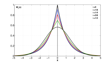
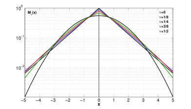
Figure 1: Plots of the symmetric $M_{\nu}$-Wright function with $\nu=0,1/8,1/4,3/8,1/2$ for $-5\leq x\leq 5$; left: linear scale, right: logarithmic scale.

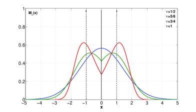
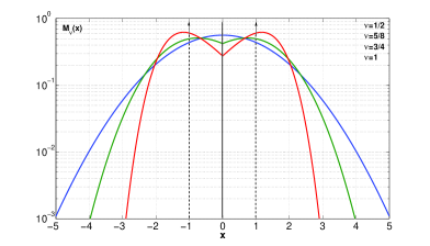
Figure 2: Plots of the symmetric $M$-Wright function with $\nu=1/2\,,\,5/8\,,\,3/4\,,\,1$ for $-5\leq x\leq 5$; left: linear scale; right: logarithmic scale.

The ${\rm I\hskip-2.0ptM}$-Wright function in two variables.

In view of the time-fractional diffusion processes that will be considered in the next Sections, it is worthwhile to introduce the function in two variables

$${\rm I\hskip-2.0ptM}_{\nu}(x,t):=t^{-\nu}\,M_{\nu}(xt^{-\nu})\,,\quad 0<\nu<1\,,\quad x,t\in\vbox{\hbox to8.9pt{I\hskip-2.1ptR\hfil}}\;^{+}\,,$$

which defines a spatial probability density in $x$ evolving in time $t$ with self-similarity exponent $H=\nu$. Of course for $x\in\vbox{\hbox to8.9pt{I\hskip-2.1ptR\hfil}}\;$ we have to consider the symmetric version obtained from (4.14) multiplying by $1/2$ and replacing $x$ by $|x|$.

Hereafter we provide a list of the main properties of this function, which can be derived from Laplace and Fourier transforms of the corresponding $M$-Wright function in one variable.

From Eq. (4.2) we derive the Laplace transform of ${\rm I\hskip-2.0ptM}_{\nu}(x,t)$ with respect to $t\in\vbox{\hbox to8.9pt{I\hskip-2.1ptR\hfil}}\;^{+}$,

$${\cal L}\left\{{\rm I\hskip-2.0ptM}_{\nu}(x,t);t\to s\right\}=s^{\nu-1}\,{\rm e}^{\displaystyle\,-xs^{\nu}}\,.$$

From Eq. (4.6) we derive the Laplace transform of ${\rm I\hskip-2.0ptM}_{\nu}(x,t)$ with respect to $x\in\vbox{\hbox to8.9pt{I\hskip-2.1ptR\hfil}}\;^{+}$,

$${\cal L}\left\{{\rm I\hskip-2.0ptM}_{\nu}(x,t);x\to s\right\}=E_{\nu}\left(-st^{\nu}\right)\,.$$

From Eq. (4.10) we derive the Fourier transform of ${\rm I\hskip-2.0ptM}_{\nu}(|x|,t)$ with respect to $x\in\vbox{\hbox to8.9pt{I\hskip-2.1ptR\hfil}}\;$,

$${\cal F}\left\{{\rm I\hskip-2.0ptM}_{\nu}(|x|,t);x\to\kappa\right\}=2E_{2\nu}\left(-\kappa^{2}t^{\nu}\right)\,.$$

Moreover, using the Mellin transform, Mainardi et al. [46] derived the following integral formula,

$${\rm I\hskip-2.0ptM}_{\nu}(x,t)=\int_{0}^{\infty}{\rm I\hskip-2.0ptM}_{\lambda}(x,\tau)\,{\rm I\hskip-2.0ptM}_{\mu}(\tau,t)\,d\tau\,,\quad\nu=\lambda\mu\,.$$

Special cases of the ${\rm I\hskip-2.0ptM}$-Wright function are simply derived for $\nu=1/2$ and $\nu=1/3$ from the corresponding ones in the complex domain, see Eqs. (3.10)-(3.11). We devote particular attention to the case $\nu=1/2$ for which we get from (4.4) the Gaussian density in IR  ,

$$\frac{1}{2}\,{\rm I\hskip-2.0ptM}_{1/2}(|x|,t)=\frac{1}{2\sqrt{\pi}t^{1/2}}\,{\rm e}^{\displaystyle\,-x^{2}/(4t)}\,.$$

For the limiting case $\nu=1$ we obtain

$$\frac{1}{2}\,{\rm I\hskip-2.0ptM}_{1}(|x|,t)=\frac{1}{2}\left[\delta(x-t)+\delta(x+t)\right]\,.$$

5 Fractional diffusion equations

Let us now consider a variety of diffusion-like equations starting from the standard diffusion equation whose fundamental solutions are expressed in terms of the $M$-Wright function depending on space and time variables. The two variables, however, turn out to be related through a self-similarity condition.

The standard diffusion equation.

The standard diffusion equation for the field $u(x,t)$ with initial condition $u(x,0)=u_{0}(x)$ is

$$\frac{\partial u}{\partial t}=K_{1}\,\frac{\partial^{2}u}{\partial x^{2}}\quad-\infty<x<\infty\,,\;t\geq 0\,,$$

where $K_{1}$ is a suitable diffusion coefficient of dimensions $[K_{1}]=[L]^{2}[T]^{-1}=cm^{2}/sec$. This initial-boundary value problem can be easily shown to be equivalent to the Volterra integral equation

$$u(x,t)=u_{0}(x)+K_{1}\int_{0}^{t}\frac{\partial^{2}u(x,\tau)}{\partial x^{2}}\,d\tau\,.$$

It is well known that the fundamental solution (usually refereed as the Green function), which is the solution corresponding to $u_{0}(x)=\delta(x)$, is the Gaussian probability density evolving in time with variance (mean square displacement) proportional to time. In our notation we hve:

$${\cal{G}}_{1}(x,t)=\frac{1}{2\sqrt{\pi K_{1}}\,t^{1/2}}\,{\rm e}^{\,\displaystyle-x^{2}/(4K_{1}t)}\,,$$

$$\sigma_{1}^{2}(t):=\int_{-\infty}^{+\infty}\!\!x^{2}\,{\cal{G}}_{1}(x,t)\,dx=2K_{1}t\,.$$

This variance law characterizes the process of normal diffusion as it emerges from Einstein’s approach to Brownian motion ($Bm$), see e.g. [68].

In view of future developments, we rewrite the Green function in terms of the $M$-Wright function by recalling Eq. (3.10), that is,

$${\cal{G}}_{1}(x,t)=\frac{1}{2}\frac{1}{\sqrt{K_{1}}\,t^{1/2}}\,M_{1/2}\left(\frac{|x|}{\sqrt{K_{1}}\,t^{1/2}}\right)\,.$$

From the self-similarity of the Green function in (5.3) or (5.5) we are led to write

$${\cal{G}}_{1}(x,t)=\frac{1}{\sqrt{K_{1}}\,t^{H}}\,{\cal{G}}_{1}\left(\frac{|x|}{\sqrt{K_{1}}\,t^{H}},1\right)\,,$$

where $H=1/2$ is the similarity (or Hurst) exponent and $\xi=|x|/(\sqrt{K_{1}}\,t^{1/2})$ acts as the similarity variable. We refer to the one-variable function ${\cal{G}}_{1}(\xi)$ as the reduced Green function.

The stretched-time standard diffusion equation.

Let us now stretch the time variable in Eq. (5.1) by replacing $t$ with $t^{\alpha}$ where $0<\alpha<2$. We have

$$\frac{\partial u}{\partial(t^{\alpha})}\ =K_{\alpha}\,\frac{\partial^{2}u}{\partial x^{2}}\,,\quad-\infty<x<+\infty\,,\;t\geq 0\,,$$

where $K_{\alpha}$ is a sort of stretched diffusion coefficient of dimensions $[K_{\alpha}]=[L]^{2}[T]^{-\alpha}=cm^{2}/sec^{\alpha}$. It is easy to recognize that such equation is akin to the standard diffusion equation but with a diffusion coefficient depending on time, $K_{1}(t)=\alpha t^{\alpha-1}\,K_{\alpha}$. In fact, using the rule

$$\frac{\partial}{\partial t^{\alpha}}=\frac{1}{\alpha t^{\alpha-1}}\frac{\partial}{\partial t}\,,$$

we have

$$\frac{\partial u}{\partial t}=\alpha t^{\alpha-1}\,K_{\alpha}\,\frac{\partial^{2}u}{\partial x^{2}}\,,\quad-\infty<x<+\infty\,,\;t\geq 0\,.$$

The integral form corresponding to Eqs. (5.7)-(5.8) reads

$$u(x,t)=u_{0}(x)+\alpha K_{\alpha}\,\int_{0}^{t}\frac{\partial^{2}u(x,\tau)}{\partial x^{2}}\tau^{\alpha-1}\,d\tau\,.$$

The corresponding fundamental solution is the stretched-time Gaussian

$${\cal{G}}_{\alpha}(x,t)=\frac{1}{2\sqrt{\pi K_{\alpha}}\,t^{\alpha/2}}\,{\rm e}^{\,\displaystyle-x^{2}/(4K_{\alpha}t^{\alpha})}=\frac{1}{2}\frac{1}{\sqrt{K_{\alpha}}\,t^{\alpha/2}}\,M_{1/2}\left(\frac{|x|}{\sqrt{K_{\alpha}}\,t^{\alpha/2}}\right)\,.$$

The corresponding variance

$$\sigma_{\alpha}^{2}(t):=\int_{-\infty}^{+\infty}\!\!x^{2}\,{\cal{G}}_{\alpha}(x,t)\,dx=2K_{\alpha}t^{\alpha}\,,$$

is characteristic of a general process of anomalous diffusion, precisely of slow diffusion for $0<\alpha<1$, and fast diffusion for $1<\alpha<2$.

The time-fractional diffusion equation.

In literature there exist two forms of the time-fractional diffusion equation of a single order, one with Riemann-Liouvile derivative and one with Caputo derivative These forms are equivalent if we refer to the standard initial condition $u(x,0)=u_{0}(x)$, as shown in [47].

Taking a real number $\beta\in(0,1)$, the time-fractional diffusion equation of order $\beta$ in the Riemann-Liouville sense reads

$$\frac{\partial u}{\partial t}={K_{\beta}}\,{D^{1-\beta}_{t}}\,\frac{\partial^{2}u}{\partial x^{2}}\,,$$

whereas in the Caputo sense reads

$${}_{*}D^{\beta}_{t}u={K_{\beta}}\,\frac{\partial^{2}u}{\partial x^{2}}\,,$$

where $K_{\beta}$ is a sort of fractional diffusion coefficient of dimensions $[K_{\beta}]=[L]^{2}[T]^{-\beta}=cm^{2}/sec^{\beta}$. Like for diffusion equations of integer order (5.1) and (5.7)-(5.8), we consider the equivalent integral equation corresponding to our fractional diffusion equations (5.12)-(5.13),

$$u(x,t)=u_{0}(x)+K_{\beta}\,\frac{1}{\Gamma(\beta)}\int_{0}^{t}(t-\tau)^{\beta-1}\,\frac{\partial^{2}u(x,\tau)}{\partial x^{2}}\,d\tau\,.$$

The Green function $\mathcal{G}_{\beta}(x,t)$ for the equivalent Eqs. (5.12)-(5.14) can be expressed, also in this case, in terms of the $M$-Wright function, as shown in Appendix by adopting two different approaches, as follows:

$$\mathcal{G}_{\beta}(x,t)=\frac{1}{2}\frac{1}{\sqrt{K_{\beta}}\,t^{\beta/2}}\,M_{\beta/2}\left(\frac{|x|}{\sqrt{K_{\beta}}\,t^{\beta/2}}\right)\,.$$

The corresponding variance can be promptly obtained from the general formula (5.5) for the absolute moment of the $M$-Wright function. In fact, using (5.5) and (5.15) and after an obvious change of variable, we obtain

$$\sigma_{\beta}^{2}(t):=\int_{-\infty}^{+\infty}\!\!x^{2}\,{\cal{G}}_{\beta}(x,t)\,dx=\frac{2}{\Gamma(\beta+1)}\,K_{\beta}\,t^{\beta}\,.$$

As a consequence, for $0<\beta<1$ the variance is consistent with a process of slow diffusion with similarity exponent $H=\beta/2$. For further reading on time-fractional diffusion equations and their solutions the reader is referred, among others, to [39, 44, 45] and [62], [66].

The stretched time-fractional diffusion equation.

In the fractional diffusion equation (5.12), let us stretch the time variable by replacing $t$ with $t^{\alpha/\beta}$ where $0<\alpha<2$ and $0<\beta\leq 1$. We have

$$\frac{\partial u}{\partial t^{\alpha/\beta}}=K_{\alpha\,\beta}\,D^{1-\beta}_{t^{\alpha/\beta}}\,\frac{\partial^{2}u}{\partial x^{2}}\,,$$

namely

$$\frac{\partial u}{\partial t}=\frac{\alpha}{\beta}t^{\alpha/\beta-1}\,K_{\alpha\,\beta}\,D^{1-\beta}_{t^{\alpha/\beta}}\,\frac{\partial^{2}u}{\partial x^{2}}\,,$$

where $K_{\alpha\,\beta}$ is a sort of stretched diffusion coefficient of dimensions $[K_{\alpha\,\beta}]=[L]^{2}[T]^{-\alpha}=cm^{2}/sec^{\alpha}$ that reduces to $K_{\alpha}$ if $\beta=1$ and to $K_{\beta}$ if $\alpha=\beta$. Integration of Eq. (5.18) gives the corresponding integral equation [57]

$$u(x,t)=u_{0}(x)+K_{\alpha\,\beta}\,\frac{1}{\Gamma(\beta)}\frac{\alpha}{\beta}\,\int_{0}^{t}\tau^{\alpha/\beta-1}\,(t^{\alpha/\beta}-\tau^{\alpha/\beta})^{\beta-1}\,\frac{\partial^{2}u(x,\tau)}{\partial x^{2}}\,d\tau\,,$$

whose Green function $\mathcal{G}_{\alpha\,\beta}(x,t)$ is

$$\mathcal{G}_{\alpha\,\beta}(x,t)=\frac{1}{2}\,\frac{1}{\sqrt{K_{\alpha\,\beta}}\,t^{\alpha/2}}\,M_{\beta/2}\left(\frac{|x|}{\sqrt{K_{\alpha\beta}}\,t^{\alpha/2}}\right)\,,$$

with variance

$$\sigma_{\alpha,\beta}^{2}(t):=\int_{-\infty}^{+\infty}\!\!x^{2}\,{\cal{G}}_{\alpha,\beta}(x,t)\,dx=\frac{2}{\Gamma(\beta+1)}\,K_{\alpha\,\beta}\,t^{\alpha}\,.$$

As a consequence, the resulting process turns out to be self-similar with Hurst exponent $H=\alpha/2$ and a variance law consistent both with slow diffusion if $0<\alpha<1$ and fast diffusion if $1<\alpha<2$. We note that the parameter $\beta$ does explicitly enter in the variance law (5.21) only in the determination of the multiplicative constant.

It is straightforward to note that the evolution equations of this process reduce to those for time-fractional diffusion if $\alpha=\beta<1$, for stretched diffusion if $\alpha\neq 1$ and $\beta=1$, and finally to standard diffusion if $\alpha=\beta=1$.

6 Fractional diffusion processes with stationary increments

We have seen that any Green function associated to the diffusion-like equations considered in the previous Section can be interpreted as the time-evolving one-point $pdf$ of certain self-similar stochastic processes. However, in general, it is not possible to define a unique (self-similar) stochastic process because the determination of any multi-point probability distribution is required, see e.g. [58].

In other words, starting from a master equation which describes the dynamic evolution of a probability density function $f(x,t)$, it is always possible to define an equivalence class of stochastic processes with the same marginal density function $f(x,t)$. All these processes provide suitable stochastic representations for the starting equation. It is clear that additional requirements may be stated in order to uniquely select the probabilistic model.

For instance, considering Eq. (5.18), the additional requirement of stationary increments, as shown by Mura et al., see [55, 56, 57, 58], can lead to a class $\{B_{\alpha,\beta}(t),\;t\geq 0\}$, called “generalized” grey Brownian motion ($ggBm$), which, by construction, is made up of self-similar processes with stationary increments and Hurst exponent $H=\alpha/2$. Thus $\{B_{\alpha,\beta}(t),\;t\geq 0\}$ is a special class of $H\!-\!sssi$ processes, which provide non-Markovian stochastic models for anomalous diffusion, both of slow type ($0<\alpha<1$) and fast type ($1<\alpha<2$).

The $ggBm$ includes some well known processes, so that it defines an interesting general theoretical framework. The fractional Brownian motion ($fBm$) appears for $\beta=1$ and is associated with Eq. (5.7); the grey Brownian motion ($gBm$), defined by Schneider [64, 65], corresponds to the choice $\alpha=\beta$, with $0<\beta<1$, and is associated to Eqs. (5.12), (5.13) or (5.14); finally, the standard Brownian motion ($Bm$) is recovered by setting $\alpha=\beta=1$ being associated to Eq. (5.1). We should note that only in the particular case of $Bm$ the corresponding process is Markovian.

In Figure 3 we present a diagram that allows to identify the elements of the $ggBm$ class. The top region $1<\alpha<2$ corresponds to the domain of fast diffusion with long-range dependence. In this domain the increments of the process $B_{\alpha,\beta}(t)$ are positively correlated, so that the trajectories tend to be more regular (persistent). It should be noted that long-range dependence is associated to a non-Markovian process which exhibits long-memory properties. The horizontal line $\alpha=1$ corresponds to processes with uncorrelated increments, which model various phenomena of normal diffusion. For $\alpha=\beta=1$ we recover the Gaussian process of the standard Brownian motion. The Gaussian process of the fractional Brownian motion is identified by the vertical line $\beta=1$. The bottom region $0<\alpha<1$ corresponds to the domain of slow diffusion. The increments of the corresponding process $B_{\alpha,\beta}(t)$ turn out to be negatively correlated and this implies that the trajectories are strongly irregular (anti-persistent motion); the increments form a stationary process which does not exhibit long-range dependence. Finally, the diagonal line ($\alpha=\beta$) represents the Schneider grey Brownian motion ($gBm$).

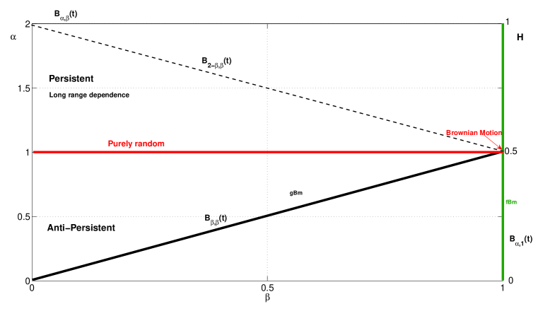
Figure 3: Parametric class of generalized grey Brownian motion

Here we want to define the $ggBm$ by making use of the Kolmogorov extension theorem and the properties of the $M$-Wright function. According to Mura and Pagnini [57], the generalized grey Brownian motion $B_{\alpha,\beta}(t)$ is a stochastic process defined in a certain probability space such that its finite-dimensional distributions are given by

$$f_{\alpha,\beta}(x_{1},x_{2},\dots,x_{n};\gamma_{\alpha,\beta})=\displaystyle\frac{(2\pi)^{-\frac{n-1}{2}}}{\sqrt{2\Gamma(1+\beta)^{n}\det{\gamma_{\alpha,\beta}}}}\int_{0}^{\infty}\frac{1}{\tau^{n/2}}M_{1/2}\left(\frac{\xi}{\tau^{1/2}}\right)M_{\beta}(\tau)d\tau,$$

with

$$\xi=\left(2\Gamma(1+\beta)^{-1}\sum_{i,j=1}^{n}x_{i}{\gamma_{\alpha,\beta}}^{-1}(t_{i},t_{j})x_{j}\right)^{1/2},$$

and covariance matrix

$$\gamma_{\alpha,\beta}(t_{i},t_{j})=\frac{1}{\Gamma(1+\beta)}(t_{i}^{\alpha}+t_{j}^{\alpha}-|t_{i}-t_{j}|^{\alpha}),\;\;i,j=1,\dots,n\,.$$

The covariance matrix (6.3) characterizes the typical dependence structure of a self-similar process with stationary increments and Hurst exponent $H=\alpha/2$, see e.g. [70].

Using Eq. (4.18), for $n=1$, Eq. (6.1) reduces to:

$$f_{\alpha,\beta}(x,t)=\displaystyle\frac{1}{\sqrt{4t^{\alpha}}}\int_{0}^{\infty}{\rm I\hskip-2.0ptM}_{1/2}\left(|x|t^{-\alpha/2},\tau\right){\rm I\hskip-2.0ptM}_{\beta}(\tau,1)\,d\tau=\frac{1}{2}t^{-\alpha/2}M_{\beta/2}(|x|t^{-\alpha/2})\,.$$

This means that the marginal density function of the $ggBm$ is indeed the fundamental solution (5.20) of Eqs. (5.17)-(5.18) with $K_{\alpha\beta}=1$. Moreover, because $M_{1}(\tau)=\delta(\tau-1)$, for $\beta=1$, putting $\gamma_{\alpha,1}\equiv\gamma_{\alpha}$, we have that Eq. (6.1) provides the Gaussian distribution of the fractional Brownian motion,

$$f_{\alpha,1}(x_{1},x_{2},\dots,x_{n};\gamma_{\alpha,1})=\displaystyle\frac{(2\pi)^{-\frac{n-1}{2}}}{\sqrt{2\det{\gamma_{\alpha}}}}M_{1/2}\left(\left(2\sum_{i,j=1}^{n}x_{i}\gamma_{\alpha}^{-1}(t_{i},t_{j})x_{j}\right)^{1/2}\right)\,,$$

which finally reduces to the standard Gaussian distribution of Brownian motion as $\alpha=1$.

By the definition used above, it is clear that, fixed $\beta$, $B_{\alpha,\beta}(t)$ is characterized only by its covariance structure, as shown by Mura et al. [56], [57]. In other words, the $ggBm$, which is not Gaussian in general, is an example of a process defined only through its first and second moments, which indeed is a remarkable property of Gaussian processes. Consequently, the $ggBm$ appears to be a direct generalization of Gaussian processes, in the same way as the $M$-Wright function is a generalization of the Gaussian function.

7 Concluding discussion

In this review paper we have surveyed a quite general approach to derive models for anomalous diffusion based on a family of time-fractional diffusion equations depending on two parameters $\alpha\in(0,2)$, $\beta\in(0,1]$.

The unifying topic of this analysis is the so-called $M$-Wright function by which the fundamental solutions of these equations are expressed. Such function is shown to exhibit fundamental analytical properties that were properly used in recent papers for characterizing and simulating a general class of self-similar stochastic processes with stationary increments including fractional Brownian motion and grey Brownian motion.

In this respect, the $M$-Wright function emerges to be a natural generalization of the Gaussian density to model diffusion processes, covering both slow and fast anomalous diffusion and including non-Markovian property. In particular, it turns out to be the main function for the special $H-sssi$ class of stochastic processes (which are self-similar with stationary increments) governed by a master equation of fractional type.

Appendix A: The fundamental solution of the time-fractional diffusion equation

The fundamental solution ${\cal{G}}_{\beta}(x,t)$ for the time-fractional diffusion equation can be obtained by applying in sequence the Fourier and Laplace transforms to any form chosen among Eqs. (5.12)-(5.14) with the initial condition ${\cal{G}}_{\beta}(x,0^{+})=u_{0}(x)=\delta(x)$. Let us devote our attention to the integral form (5.14) using non-dimensional variables by setting $K_{\beta}=1$ and adopting the notation $J_{t}^{\beta}$ for the fractional integral. Then, our Cauchy problem reads

$${\cal{G}}_{\beta}(x,t)=\delta(x)+J_{t}^{\beta}\,\frac{\partial^{2}{\cal{G}}_{\beta}}{\partial x^{2}}(x,t)\,.$$

In the Fourier-Laplace domain, after applying formula (2.18) for the Laplace transform of the fractional integral and observing $\widehat{\delta}(\kappa)\equiv 1$, see e.g. [15], we get

$$\widehat{\widetilde{G_{\beta}}}(\kappa,s)=\frac{1}{s}-\frac{\kappa^{2}}{s^{\beta}}\,\widehat{\widetilde{G_{\beta}}}(\kappa,s)\,,$$

from which

$$\widehat{\widetilde{{\cal{G}}_{\beta}}}(\kappa,s)=\frac{s^{\beta-1}}{s^{\beta}+\kappa^{2}}\,,\quad 0<\beta\leq 1\,,\quad\Re(s)>0\,,\;\kappa\in\vbox{\hbox to8.9pt{I\hskip-2.1ptR\hfil}}\;\,.$$

To determine the Green function ${\cal{G}}_{\beta}(x,t)$ in the space-time domain we can follow two alternative strategies related to the order in carrying out the inversions in (A.2).
(S1) : invert the Fourier transform getting $\widetilde{{\cal{G}}_{\beta}}(x,s)$ and then invert the remaining Laplace transform;
(S2) : invert the Laplace transform getting $\widehat{G_{\beta}}(\kappa,t)$ and then invert the remaining Fourier transform.

Strategy (S1): Recalling the Fourier transform pair

$$\frac{a}{b+\kappa^{2}}\,\,\stackrel{{\scriptstyle{\cal F}}}{{\leftrightarrow}}\,\,\frac{a}{2b^{1/2}}\,{\rm e}^{\displaystyle\,-|x|b^{1/2}}\,,\quad a,b>0\,,$$

and setting $a=s^{\beta-1}$, $b=s^{\beta}$, we get

$$\widetilde{{\cal{G}}_{\beta}}(x,s)=\frac{1}{2}s^{\beta/2-1}\,{\rm e}^{\displaystyle\,-|x|s^{\beta/2}}\,.$$

Strategy (S2): Recalling the Laplace transform pair

$$\frac{s^{\beta-1}}{s^{\beta}+c}\,\,\stackrel{{\scriptstyle{\cal L}}}{{\leftrightarrow}}\,\,E_{\beta}(-ct^{\beta})\,,\quad c>0\,,$$

and setting $c=\kappa^{2}$, we have

$$\widehat{G_{\beta}}(\kappa,t)=E_{\beta}(-\kappa^{2}t^{\beta})\,.$$

Both strategies lead to the result

$${\cal{G}}_{\beta}(x,t)=\frac{1}{2}{\rm I\hskip-2.0ptM}_{\beta/2}(|x|,t)=\frac{1}{2}\,t^{-\beta/2}\,M_{\beta/2}\left(\frac{|x|}{t^{\beta/2}}\right)\,,$$

consistent with Eq. (5.15). Here we have used the ${\rm I\hskip-2.0ptM}$-Wright function, introduced in Section 4, and its properties related to the Laplace transform pair (4.15) for inverting (A.4) and the Fourier transform pair (4.17) for inverting (A.6).

Appendix B: The fundamental solution of the time-fractional drift equation

Let us finally note that the $M$-Wright function does appear also in the fundamental solution of the time-fractional drift equation. Writing this equation in non-dimensional form and adopting the Caputo derivative we have

$${}_{*}D^{\beta}_{t}u(x,t)=-\frac{\partial}{\partial x}u(x,t)\,,\quad-\infty<x<+\infty\,,\;t\geq 0\,,$$

where $0<\beta<1$ and $u(x,0^{+})=u_{0}(x)$. When $u_{0}(x)=\delta(x)$ we obtain the fundamental solution (Green function) that we denote by ${\cal{G}}_{\beta}^{*}(x,t)$. Following the approach of Appendix A, we show that

$${\cal{G}}_{\beta}^{*}(x,t)=\left\{\begin{array}[]{ll}{\displaystyle t^{-\beta}\,M_{\beta}\left(\frac{x}{t^{\beta}}\right)}\,,&x>0\,,\\ 0\,,&x<0\,,\end{array}\right.$$

that for $\beta=1$ reduces to the right running pulse $\delta(x-t)$ for $x>0$.

In the Fourier-Laplace domain, after applying formula (2.19) for the Laplace transform of the Caputo fractional derivative and observing $\widehat{\delta}(\kappa)\equiv 1$, see e.g. [15], we get

$$s^{\beta}\,\widehat{\widetilde{G_{\beta}^{*}}}(\kappa,s)-s^{\beta-1}=+i\kappa\,\widehat{\widetilde{G_{\beta}^{*}}}(\kappa,s)\,,$$

from which

$$\widehat{\widetilde{{\cal{G}}_{\beta}^{*}}}(\kappa,s)=\frac{s^{\beta-1}}{s^{\beta}-i\kappa}\,,\quad 0<\beta\leq 1\,,\quad\Re(s)>0\,,\;\kappa\in\vbox{\hbox to8.9pt{I\hskip-2.1ptR\hfil}}\;\,.$$

Like in Appendix A, to determine the Green function ${\cal{G}}_{\beta}^{*}(x,t)$ in the space-time domain we can follow two alternative strategies related to the order in carrying out the inversions in (B.3).
(S1) : invert the Fourier transform getting $\widetilde{{\cal{G}}_{\beta}}(x,s)$ and then invert the remaining Laplace transform;
(S2) : invert the Laplace transform getting $\widehat{G_{\beta}^{*}}(\kappa,t)$ and then invert the remaining Fourier transform.

Strategy (S1): Recalling the Fourier transform pair

$$\frac{a}{b-i\kappa}\,\,\stackrel{{\scriptstyle{\cal F}}}{{\leftrightarrow}}\,\,\frac{a}{b}\,{\rm e}^{\displaystyle\,-xb}\,,\quad a,b>0\,,\;x>0\,,$$

and setting $a=s^{\beta-1}$, $b=s^{\beta}$, we get

$$\widetilde{{\cal{G}}_{\beta}^{*}}(x,s)=s^{\beta-1}\,{\rm e}^{\displaystyle\,-xs^{\beta}}\,.$$

Strategy (S2): Recalling the Laplace transform pair

$$\frac{s^{\beta-1}}{s^{\beta}+c}\,\,\stackrel{{\scriptstyle{\cal L}}}{{\leftrightarrow}}\,\,E_{\beta}(-ct^{\beta})\,,\quad c>0\,,$$

and setting $c=-i\kappa$, we have

$$\widehat{G_{\beta}^{*}}(\kappa,t)=E_{\beta}(i\kappa t^{\beta})\,.$$

Both strategies lead to the result (B.2).

In view of Eq. (4.1) we also recall that the $M$-Wright function is related to the unilateral extremal stable density of index $\beta$. Then, using our notation stated in [44] for stable densities, we write our Green function as

$${\cal{G}}_{\beta}^{*}(x,t)=\frac{t}{\beta}\,x^{-1-1/\beta}\,L_{\beta}^{-\beta}\left(tx^{-1/\beta}\right)\,,$$

To conclude this Appendix let us briefly discuss the above results in view of their relevance in fractional diffusion processes following the recent paper by Gorenflo and Mainardi [22]. Equation (B.1) describes the evolving sojourn probability density of the positively oriented time-fractional drift process of a particle, starting in the origin at the instant zero. It has been derived in [22] as a properly scaled limit for the evolution of the counting number of the Mittag-Leffler renewal process (the fractional Poisson process). It can be given in several forms, and often it is cited as the subordinator (producing the operational time from the physical time) for space-time-fractional diffusion as in the form (B.8). For more details see [25], where simulations of space-time-fractional diffusion processes have been considered as composed by time-fractional and space-fractional diffusion processes.

This analysis can be compared to that described with a different language in papers by Meerschaert et al. [51, 52]. Recently, a more exhaustive analysis has been given by Gorenflo [17].

References

- [1] B.N.N. Achar, J.W. Hanneken and T. Clarke, Damping characteristics of a fractional oscillator, Physica A 339 (2004), 311–319.
- [2] R. Balescu, V-Langevin equations, continuous time random walks and fractional diffusion, Chaos, Solitons and Fractals 34 (2007), 62-80.
- [3] C.M. Bender and S.A. Orszag, Advanced Mathematical Methods for Scientists and Engineers, McGraw-Hill, Singapore (1987).
- [4] P.W. Buchen and F. Mainardi, Asymptotic expansions for transient viscoelastic waves, Journal de Mécanique 14 (1975), 597-608.
- [5] M. Caputo, Linear models of dissipation whose is almost frequency independent, Part II. Geophys. J. Roy. Astronom. Soc. 13 (1967), 529–539.
- [6] M. Caputo, Elasticity and Dissipation Zanichelli, Bologna (1969). [in Italian]
- [7] A.V. Chechkin, R. Gorenflo and I.M. Sokolov, Retarding subdiffusion and accelerating superdiffusion governed by distributed-order fractional diffusion equations. Phys. Rev. E 66 (2002) 046129/1-6.
- [8] A.V. Chechkin, R. Gorenflo, I.M. Sokolov and V.Yu. Gonchar, Distributed order time fractional diffusion equation. Fractional Calculus and Applied Analysis 6 (2003), 259-279.
- [9] A.V. Chechkin, V.Yu. Gonchar, R. Gorenflo, N. Korabel and I.M. Sokolov, Generalized fractional diffusion equations for accelerating subdiffusion and truncated Lévy flights, Phys. Rev. E 78 (2008), 021111/1-13.
- [10] G. Doetsch, Introduction to the Theory and Applications of the Laplace Transformation, Springer Verlag, Berlin (1974).
- [11] A.A. Dubkov, B. Spagnolo and V.V. Uchaikin, Lévy flight superdiffusion: an introduction, Int. Journal of Bifurcation and Chaos 18 No 9 (2008), 2649–2671.
- [12] A. Erdélyi, W. Magnus, F. Oberhettinger and F.G. Tricomi, Higher Transcendental Functions, Vol. 3, Ch. 18, McGraw-Hill, New-York (1954).
- [13] W. Feller, An Introduction to Probability Theory and its Applications, Vol. 2, 2-nd edn., Wiley, New York (1971). [1-st edn. 1966]
- [14] A. Freed, K. Diethelm and Yu. Luchko, Fractional-order Viscoelasticity (FOV): Constitutive Development using the Fractional Calculus, First Annual Report, NASA/TM-2002-211914, Gleen Research Center (2002), pp. XIV – 121.
- [15] I.M. Gel`fand and G.E. Shilov, Generalized Functions, Volume I. Academic Press, New York and London (1964).
- [16] G. Germano, M. Politi, E. Scalas and R.E. Schilling, Stochastic calculus for uncoupled continuous-time random walks, Phys. Rev. E 79 (2009), 066102/1–12.
- [17] R. Gorenflo, Mittag-Leffler waiting time, power laws, rarefaction, continuous time random walk, diffusion limit, Unpublished lecture, Workshop on Fractional Calculus and Statistical Distributions, November 25–27, 2009, Centre for Mathematical Sciences, Pala Campus, Pala-Kerala, India.
- [18] R. Gorenflo, J. Loutchko and Yu. Luchko, Computation of the Mittag-Leffler function and its derivatives, Fractional Calculus and Applied Analysis 5 (2002), 491–518.
- [19] R. Gorenflo, Yu. Luchko and F. Mainardi, Analytical properties and applications of the Wright function. Fractional Calculus and Applied Analysis 2 (1999), 383–414. E-print http://arxiv.org/abs/math-ph/0701069
- [20] R. Gorenflo, Yu. Luchko and F. Mainardi, Wright functions as scale–invariant solutions of the diffusion–wave equation. J. Computational and Applied Mathematics 118 (2000), 175–191.
- [21] R. Gorenflo and F. Mainardi, Fractional calculus: integral and differential equations of fractional order. In A. Carpinteri and F. Mainardi (Editors), Fractals and Fractional Calculus in Continuum Mechanics. Springer Verlag, Wien and New York (1997), pp. 223–276. E-print: http://arxiv.org/abs/0805.3823
- [22] R. Gorenflo and F. Mainardi, Continuous time random walk, Mittag-Leffler waiting time and fractional diffusion: mathematical aspects, In R. Klages, G. Radons and I.M. Sokolov (Editors), Anomalous Transport: Foundations and Applications, Wiley-VCH, Weinheim, Germany, 2008, Chap. 4, pp. 93-127. E-print: http://arxiv.org/abs/0705.0797
- [23] R. Gorenflo, F. Mainardi, D. Moretti and P. Paradisi, Time-fractional diffusion: a discrete random walk approach, Nonlinear Dynamics 29 (2002), 129-143.
- [24] R. Gorenflo, F. Mainardi, D. Moretti, G. Pagnini and P. Paradisi, Discrete random walk models for space time fractional diffusion, Chem. Phys. 284 (2002), 521-541.
- [25] R. Gorenflo, F. Mainardi and A. Vivoli, Continuous time random walk and parametric subordination in fractional diffusion, Chaos, Solitons and Fractals 34 (2007), 87–103. E-print http://arxiv.org/abs/cond-mat/0701126
- [26] A. Hanyga, Multi-dimensional solutions of time-fractional diffusion-wave equation, Proc. R. Soc. London 458 (2002), 933-957.
- [27] P. Humbert, Nouvelles correspondances symboliques, Bull. Sci. Mathém. (Paris, II ser.) 69 (1945), 121–129.
- [28] A.A. Kilbas, M. Saigo and J.J. Trujillo, On the generalized Wright function. Fractional Calculus and Applied Analysis 5 (2002), 437–460.
- [29] A.A. Kilbas, H.M. Srivastava and J.J. Trujillo, Theory and Applications of Fractional Differential Equations, Elsevier, Amsterdam (2006).
- [30] V. Kiryakova, Generalized Fractional Calculus and Applications. Longman, Harlow (1994). [Pitman Research Notes in Mathematics, Vol. 301]
- [31] V. Kiryakova, The multi-index Mittag-Leffler functions as important class of special functions of fractional calculus, Computers and Mathematics with Applications (2009a), in press: doi:10.1016/j.camwa.2009.08.025
- [32] V. Kiryakova, The special functions of fractional calculus as generalized fractional calculus operators of some basic functions, Computers and Mathematics with Applications (2009b), in press: doi:10.1016/j.camwa.2009.05.014
- [33] F. Liu, S. Shen, V. Anh and I. Turner, Analysis of a discrete non-Markovian random walk approximation for the time fractional diffusion equation, ANZIAM Journal E 46 (2005), 488–504.
- [34] F. Liu, P. Zhuang, V. Anh, I. Turner and K. Burrage, Stability and convergence of the difference methods for the space-time fractional advection-diffusion equation, Appl. Math. Comp. 191 No 1 (2007), 12–20.
- [35] Yu. Luchko, Algorithms for evaluation of the Wright function for the real arguments’ values, Fractional Calculus and Applied Analysis 11 (2008), 57–75.
- [36] F. Mainardi, On the initial value problem for the fractional diffusion-wave equation, In S. Rionero and T. Ruggeri (Editors), Waves and Stability in Continuous Media, World Scientific, Singapore (1994), pp. 246–251.
- [37] F. Mainardi, The fundamental solutions for the fractional diffusion-wave equation. Applied Mathematics Letters 9 No 6 (1996), 23–28.
- [38] F. Mainardi, Fractional relaxation-oscillation and fractional diffusion-wave phenomena. Chaos, Solitons and Fractals 7 (1996), 1461–1477.
- [39] F. Mainardi, Fractional calculus: some basic problems in continuum and statistical mechanics. In A. Carpinteri and F. Mainardi (Editors), Fractals and Fractional Calculus in Continuum Mechanics. Springer Verlag, Wien and New York (1997), pp. 291-348. [http://www.fracalmo.org]
- [40] F. Mainardi, Fractional Calculus and Waves in Linear Viscoelasticity Imperial College Press, London (2010), forthcoming.
- [41] F. Mainardi and R. Gorenflo, On Mittag-Leffler-type functions in fractional evolution processes. J. Computational and Applied Mathematics 118 (2000), 283–299.
- [42] F. Mainardi and R. Gorenflo, Time-fractional derivatives in relaxation processes: a tutorial survey, Fractional Calculus and Applied Analysis 10 No 3 (2007), 269–308. E-print http://arxiv.org/abs/0801.4914
- [43] F. Mainardi, R. Gorenflo and A. Vivoli, Renewal processes of Mittag-Leffler and Wright type, Fractional Calculus and Applied Analysis 8 (2005), 7–38. E-print: http://arxiv.org/abs//0701455
- [44] F. Mainardi, Yu. Luchko and G. Pagnini, The fundamental solution of the space-time fractional diffusion equation. Fractional Calculus and Applied Analysis 4 (2001), 153–192. E-print: http://arxiv.org/abs/cond-mat/0702419
- [45] F. Mainardi and G. Pagnini, The Wright functions as solutions of the time-fractional diffusion equations, Applied Mathematics and Computation 141 (2003), 51–62.
- [46] F. Mainardi, G. Pagnini and R. Gorenflo, Mellin transform and subordination laws in fractional diffusion processes, Fractional Calculus and Applied Analysis 6 (2003), 441–459. E-print: http://arxiv.org/abs/math/0702133
- [47] F. Mainardi, G. Pagnini and R. Gorenflo, Some aspects of fractional diffusion equations of single and distributed order, Applied Mathematics and Computation 187 (2007), 295–305. E-print: http://arxiv.org/abs/0711.4261
- [48] F. Mainardi and M. Tomirotti, On a special function arising in the time fractional diffusion-wave equation. In P. Rusev, I. Dimovski and V. Kiryakova (Editors), Transform Methods and Special Functions, Sofia 1994, Science Culture Technology Publ., Singapore(1995), pp. 171–183.
- [49] F. Mainardi and M. Tomirotti, Seismic pulse propagation with constant and stable probability distributions, Annali di Geofisica 40 (1997), 1311–1328.
- [50] B.B. Mandelbrot and J.W. Van Ness, Fractional Brownian motions, fractional noises and applications, SIAM Rev. 10 (1968), 422-433.
- [51] M.M. Meerschaert, D.A. Benson, H.P. Scheffler, and B. Baeumer, Stochastic solution of space-time fractional diffusion equations, Physical Review E 65 No 4 (2002), 1103–1106.
- [52] M.M. Meerschaert and H.-P. Scheffler, Limit theorems for continuous-time random walks with infinite mean waiting times. J. Appl. Prob. 41 (2004), 623–638.
- [53] R. Metzler and J. Klafter, The random walk’s guide to anomalous diffusion: a fractional dynamics approach. Physics Reports 339 (2000), 1–77.
- [54] J. Mikusiński, On the function whose Laplace transform is Studia Math. 18 (1959), 191–198.
- [55] A. Mura, Non-Markovian Stochastic Processes and their Applications: from Anomalous Diffusion to Time Series Analysis, PhD Thesis in Physics, University of Bologna, Department of Physics, March (2008). Supervisor Prof. F. Mainardi. The PhD thesis is available at http://www.fracalmo.org/mura/
- [56] A. Mura and F. Mainardi, A class of self-similar stochastic processes with stationary increments to model anomalous diffusion in physics, Integral Transforms and Special Functions 20 No 3/4 (2009), 185–198. E-print: http://arxiv.org/abs/0711.0665
- [57] A. Mura and G. Pagnini, Characterizations and simulations of a class of stochastic processes to model anomalous diffusion, Journal of Physics A: Math. Theor. 41 No 28 (2008), 285002/1–22. E-print http://arxiv.org/abs/0801.4879
- [58] A. Mura, M.S. Taqqu and F. Mainardi: Non-Markovian diffusion equations and processes: analysis and simulation, Physica A 387 (2008), 5033–5064. E-print: http://arxiv.org/abs/0712.0240
- [59] I. Podlubny, Fractional Differential Equations. Academic Press, San Diego (1999).
- [60] I. Podlubny, Mittag-Leffler function. The MATLAB routine is available from the WEB site http://www.mathworks.com/matlabcentral/fileexchange
- [61] H. Pollard, The representation of as a Laplace integral, Bull. Amer. Math. Soc. 52 (1946), 908–910.
- [62] A.I. Saichev and G.M. Zaslavsky, Fractional kinetic equations: solutions and applications. Chaos 7 (1997), 753–764.
- [63] E. Scalas, R. Gorenflo and F. Mainardi, Uncoupled continuous-time random walks: solution and limiting behaviour of the master equation. Physical Review E 69 (2004), 011107/1-8.
- [64] W.R. Schneider, Grey noise, in: S. Albeverio, G. Casati, U. Cattaneo, D. Merlini and R. Moresi (Editors), Stochastic Processes, Physics and Geometry, World Scientific, Singapore (1990), pp. 676-681.
- [65] W.R. Schneider, Grey noise, in: S. Albeverio, J.E. Fenstad, H. Holden, T. Lindstrøm (Editors), Ideas and Methods in Mathematical Analysis, Stochastics and Applications, Vol 1, Cambridge University Press, Cambridge (1990), pp. 261-282.
- [66] W.R. Schneider and W. Wyss, Fractional diffusion and wave equations. J. Math. Phys. 30 (1989), 134–144.
- [67] H.J. Seybold and R. Hilfer, Numerical results for the generalized Mittag-Leffler function, Fractional Calculus and Applied Analysis 8 (2005), 127–139.
- [68] I.M. Sokolov and J. Klafter, From diffusion to anomalous diffusion: A century after Einstein’s Brownian motion, Chaos 15 (2005), 026103/1-7.
- [69] B. Stankovic̀, On the function of E.M. Wright. Publ. de l’Institut Mathèmatique, Beograd, Nouvelle Sèr. 10 (1970), 113–124.
- [70] M.S. Taqqu, Fractional Brownian motion and long-range dependence, in: P. Doukan, G. Oppenheim and M.S. Taqqu (Editors), Long-range Dependence: Theory and Applications, Birkäuser, Basel and Boston (2003), pp. 5–38.
- [71] R. Wong and Y.-Q. Zhao, Smoothing of Stokes’ discontinuity for the generalized Bessel function, Proc. R. Soc. London A 455 (1999), 1381–1400.
- [72] R. Wong and Y.-Q. Zhao, Smoothing of Stokes’ discontinuity for the generalized Bessel function II, Proc. R. Soc. London A 455 (1999), 3065–3084.
- [73] E.M. Wright, On the coefficients of power series having exponential singularities, Journal London Math. Soc. 8 (1933), 71–79.
- [74] E.M. Wright, The asymptotic expansion of the generalized Bessel function, Proc. London Math. Soc. (Ser. II) 38 (1935), 257–270.
- [75] E.M. Wright, The asymptotic expansion of the generalized hypergeometric function, Journal London Math. Soc. 10 (1935), 287–293.
- [76] E.M. Wright, The generalized Bessel function of order greater than one, Quart. J. Math., Oxford ser. 11 (1940), 36–48.
- [77] Y. Zhang, D.A. Benson, M.M. Meerschaert, H.P. Scheffler, On using random walks to solve the space-fractional advection-dispersion equations, Journal of Statistical Physics 123 No 1 (2006), 89–110.
- [78] P. Zhuang and F. Liu, Implicit difference approximations for the time fractional diffusion equation, J. Appl. Math. Comput. 22 No 3 (2006), 87-99.