A two-dimensional arrangement of toothpicks is constructed by the following iterative procedure. At stage $1$, place a single toothpick of length $1$ on a square grid, aligned with the $y$-axis. At each subsequent stage, for every exposed toothpick end, place a perpendicular toothpick centered at that end. The resulting structure has a fractal-like appearance. We will analyze the toothpick sequence, which gives the total number of toothpicks after $n$ steps. We also study several related sequences that arise from enumerating active cells in cellular automata. Some unusual recurrences appear: a typical example is that instead of the Fibonacci recurrence, which we may write as $a(2+i)=a(i)+a(i+1)$, we set $n=2^{k}+i$ ($0\leq i<2^{k}$), and then $a(n)=a(2^{k}+i)=2a(i)+a(i+1)$. The corresponding generating functions look like $\prod_{k\geq 0}(1+x^{2^{k}-1}+2x^{2^{k}})$ and variations thereof.

Keywords: cellular automata (CA), enumeration, Holladay-Ulam CA, Schrandt-Ulam CA, Ulam-Warburton CA, Rule 942, Sierpiński triangle

AMS 2000 Classification: Primary 11B85

1 Introduction

We start with an infinite sheet of graph paper and an infinite supply of line segments of length $1$, called “toothpicks.” At stage $1$, we place a toothpick on the $y$-axis and centered at the origin. Each toothpick we place has two ends, and an end is said to be “exposed” if this point on the plane is neither the end nor the midpoint of any other toothpick.

At each subsequent stage, for every exposed toothpick end, we place a toothpick centered at that end and perpendicular to that toothpick. The toothpicks placed at odd-numbered stages are therefore all parallel to the $y$-axis, while those placed at even-numbered stages are parallel to the $x$-axis.

Fig. 1 shows the first ten stages of the evolution of the toothpick structure and Figs. 2, 3 show the structure after respectively $53$ and $64$ stages.

Figure 1: First ten stages of the evolution of the toothpick structure. The numbers of toothpicks in the successive stages, $T(1),\ldots,T(10)$, are $1,3,7,11,15,23,35,43,47,55$.

Figure 2: The toothpick structure after 53 stages (there are $T(53)=1379$ toothpicks).

Figure 3: The toothpick structure after 64 stages (there are $T(64)=2731$ toothpicks).

Let $t(n)$ ($n\geq 1$) denote the number of toothpicks added at the $n$th stage, with $t(0)=0$, and let $T(n):=\sum_{i=0}^{n}t(i)$ be the total number of toothpicks after $n$ stages. The initial values of $t(n)$ and $T(n)$ are shown in Table 1. These two sequences respectively form entries A139251 and A139250 in [8].

$$\begin{array}[]{|c|rrrrrrrrrr|}\hline\cr n&0&1&2&3&4&5&6&7&8&9\\ t(n)&0&1&2&4&4&4&8&12&8&4\\ T(n)&0&1&3&7&11&15&23&35&43&47\\ \hline\cr n&10&11&12&13&14&15&16&17&18&19\\ t(n)&8&12&12&16&28&32&16&4&8&12\\ T(n)&55&67&79&95&123&155&171&175&183&195\\ \hline\cr n&20&21&22&23&24&25&26&27&28&29\\ t(n)&12&16&28&32&20&16&28&36&40&60\\ T(n)&207&223&251&283&303&319&347&383&423&483\\ \hline\cr n&30&31&32&33&34&35&36&37&38&39\\ t(n)&88&80&32&4&8&12&12&16&28&32\\ T(n)&571&651&683&687&695&707&719&735&763&795\\ \hline\cr n&40&41&42&43&44&45&46&47&48&49\\ t(n)&20&16&28&36&40&60&88&80&36&16\\ T(n)&815&831&859&895&935&995&1083&1163&1199&1215\\ \hline\cr\end{array}$$

Table 1: The toothpick sequences $t(n)$ and $T(n)$ for $0\leq n\leq 49$.

The first question is, what are the numbers $t(n)$ and $T(n)$? We start by finding recurrences that they satisfy. As the number of stages grows, the array of toothpicks has a recursive, fractal-like structure, as suggested by Figs. 1, 2, 3. (For a dramatic illustration of the fractal structure, see the movie linked to entry A139251 in [8].) In order to analyze this structure, we consider a variant, the “corner” sequence, which starts from a half-toothpick protruding from one quadrant of the plane. In §2 we establish a recurrence for the corner sequence (Theorem 1) and in §3 we use this to find recurrences for $t(n)$ and $T(n)$ (Theorem 2, Corollary 3). Section §4 gives a similar recurrence for the number of squares and rectangles that are created in the toothpick structure at the $n$th stage, and §5 gives a more precise description of the fractal-like behavior and discusses the asymptotic growth of $T(n)$.

The recurrences make it easy to compute a large number of values of $t(n)$ and $T(n)$, so in a sense the initial problem has now been solved.

However, the toothpick structure is reminiscent of another, simpler, two-dimensional structure, the arrangement of square cells produced by the Ulam-Warburton cellular automaton (Ulam [17], Singmaster [13], Stanley and Chapman [15], Wolfram [22, p. 928]). For this structure there is an explicit formula for the number of ${\tt ON}$ cells at the $n$th stage, and a simple generating function for these numbers, as we will see in §6, Theorem 6.

This hint led us to look for a similar generating function and an explicit formula for the toothpick sequence. Our first attempt was a failure, but provided an surprising connection with the Sierpiński triangle, described in §7.

The generating functions for the toothpick sequence and for a number of related sequences have an interesting form: they can be written as

$$x(\alpha+\beta x)\prod_{k\geq\varepsilon}(1+\gamma x^{2^{k}-1}+\delta x^{2^{k}})\,,$$ (1)

for appropriate integers $\alpha,\beta,\gamma,\delta,\varepsilon$. In §8 we describe the relationship between such generating functions and recurrences for the underlying sequence (Theorem 7). The generating function for the toothpick sequence is then established in Theorem 8.

Generating functions of the form $\prod_{k\geq 1}(1+g_{k}x^{k})$ have been used in combinatorics and number theory for a long time (for a survey see [5]), but generating functions of the form (1) may be new—at least, until the commencement of this work, there were essentially no examples among the 170,000 entries in [8].

The following section, §9, gives a general method for obtaining explicit formulas from the generating functions (Theorem 9), and the particular formula for the toothpick sequence is given in Theorem 10.

Both the toothpick structure and the Ulam-Warburton structure are examples of cellular automata defined on graphs, and we discuss this general framework in §10. We have not been able to find much earlier work on the enumeration of active cells in cellular automata—the Stanley and Chapman American Mathematical Monthly problem [15] and the Singmaster article [13] being exceptions. We would appreciate hearing of any references we have overlooked.

Of course, two well-known examples show that one cannot hope to enumerate the active states in arbitrary cellular automata: the one-dimensional cellular automaton defined by Wolfram’s “Rule $30$” [19], [20], [22] behaves chaotically, and the two-dimensional cellular automaton corresponding to Conway’s “Game of Life” [2] is a universal Turing machine.

However, we were able to apply our techniques (with varying degrees of success) to a number of other cellular automata defined on graphs, and the last four sections discuss some of these. Section 11 discusses a structure built using T-shaped toothpicks. Sections 12-14 discusses variations on the Ulam-Warburton cellular automaton. Section 12 deals with the “Maltese cross” or Holladay-Ulam structure studied in [17], as well as some other structures mentioned in that paper. Section 13 considers what happens if we change the rule for the Ulam-Warburton cellular automaton of §6 so that a cell is turned ${\tt ON}$ if and only if one or four of its neighbors is ${\tt ON}$. The final section (§14) discusses what happens if we change the definition of the Ulam-Warburton cellular automaton to allow all eight neighbors of a square to affect the next stage. There is another variation that could have been included here, in which the rule is that a cell changes state if exactly one of its four neighbors is ${\tt ON}$. Again we have a formula for the number of $ON$ cells after $n$ generations—see entries A079315, A079317 in [8]. Many further examples of sequences based on generalized toothpick structures and cellular automata are listed in [14].

Notation.

Our cellular automata are synchronous, and we normally use the symbol $n$ to index the successive stages. Cells are either ${\tt ON}$ or ${\tt OFF}$. In all the examples we consider here, once a cell is ${\tt ON}$ it stays ${\tt ON}$. Lower case letters (e.g. $a(n)$) will denote the number of toothpicks added, or cells whose state is changed from ${\tt OFF}$ to ${\tt ON}$, at the $n$th stage, and the corresponding upper case letters (e.g. $A(n)$) will denote the total number of toothpicks or ${\tt ON}$ cells after $n$ stages (the partial sums of the $a(n)$). By the generating function for a sequence $a(n)$ (say), we will always mean the ordinary generating function ${\mathcal{A}}(x):=\sum_{n=0}^{\infty}a(n)x^{n}$. If ${\mathcal{A}}(x)$ is the generating function for $a(n)$, then ${\mathcal{A}}(x)/(1-x)$ is the generating function for $A(n)$.

Remarks.

1. A common dilemma in combinatorics is whether to index the first counting step with $n=0$ or $n=1$. In this paper we have consistently started the enumerations with zero objects (toothpicks or ${\tt ON}$ cells) at stage $0$, adding the initial object at stage $1$. This seems natural, and is the indexing used for most of these sequences in [8]. On the other hand, this is responsible for the leading factor of $x$ in the generating functions (1), (15), (17), etc., and for the fact that in the recurrences (2), (4), etc., the exceptional cases occur at the beginning of each block of $2^{k}$ terms, rather than at the end. If they had occurred at the ends of the blocks, the beginnings of all the blocks would have agreed, which would have made the triangular arrays such as that in Table 3 look rather nicer (compare Table 7). Probably there is no perfect solution to the problem, and so we have followed the indexing used in [8].

2. Reference [8] contains several hundred sequences related to the toothpick problem, many more than could be mentioned here. For a full list see [14] and also the entries in the index to [8] under “cellular automata.”

3. The computer language Mathematica® [21] has a collection of commands that can often be used to display structures produced by cellular automata and to count the ${\tt ON}$ states. For example, the command

Map[Function[Apply[Plus,Flatten[#1]]],CellularAutomaton[{
        686,{2,{{0,2,0},{2,1,2},{0,2,0}}},{1,1}},{{{1}},0},200]]

produces the first 200 terms of the sequence $U(n)$ giving the number of ${\tt ON}$ states in the Ulam-Warburton cellular automaton discussed in §6.

Figure 4: Stages $0$ through $7$ of the evolution of the corner structure. The numbers of toothpicks in the successive stages, $C(0),\ldots,C(7)$, are $0,1,3,6,9,13,20,28$.

2 The corner sequence

In order to understand the toothpick structure, it is helpful to first consider what happens if one quadrant of the plane is excluded. We impose the rule that no toothpick may cross into the third quadrant of the plane, and only ends of toothpicks may touch the negative $x$- or $y$-axes. At stage $0$, we place a half-toothpick extending horizontally from the origin to the point $(\frac{1}{2},0)$. The structure is then allowed to grow using the rule for the original toothpick sequence. The corner sequence is relevant because it describes how the main toothpick structure grows.

Let $c(n)$ ($n\geq 1$) denote the number of toothpicks added at the $n$th stage, with $c(0)=0$, and let $C(n):=\sum_{i=0}^{n}c(i)$ be the total number of toothpicks after $n$ stages. These are respectively entries A152980 and A153006 in [8].

Fig. 4 shows stages $0$ through $7$ of the evolution of the corner structure. Note that the first toothpick added, at stage $1$ (with midpoint at the end of the initial half-toothpick), matches the initial toothpick of the original toothpick sequence, except that it is shifted a half-unit to the left. The initial values of $c(n)$ and $C(n)$ are shown in Table 2.

$$\begin{array}[]{|c|rrrrrrrrrr|}\hline\cr n&0&1&2&3&4&5&6&7&8&9\\ c(n)&0&1&2&3&3&4&7&8&5&4\\ C(n)&0&1&3&6&9&13&20&28&33&37\\ \hline\cr n&10&11&12&13&14&15&16&17&18&19\\ c(n)&7&9&10&15&22&20&9&4&7&9\\ C(n)&44&53&63&78&100&120&129&133&140&149\\ \hline\cr n&20&21&22&23&24&25&26&27&28&29\\ c(n)&10&15&22&21&14&15&23&28&35&52\\ C(n)&159&174&196&217&231&246&269&297&332&384\\ \hline\cr n&30&31&32&33&34&35&36&37&38&39\\ c(n)&64&48&17&4&7&9&10&15&22&21\\ C(n)&448&496&513&517&524&533&543&558&580&601\\ \hline\cr\end{array}$$

Table 2: The corner sequences $c(n)$ and $C(n)$ for $0\leq n\leq 39$.

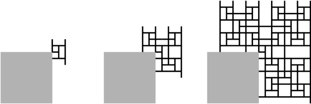
Figure 5: The corner toothpick structure after $2^{k}-1$ stages, for $k=2,3,4$.

An examination of Fig. 4 and pictures of later stages in the evolution reveals that after $2^{k}-1$ stages (for $k\geq 2$) the structure consists of an essentially solid rectangle of toothpicks with one quadrant removed. The first few cases are shown in Figs. 5. More precisely, we have:

Theorem 1

After $2^{k}-1$ stages, for $k\geq 2$, the corner toothpick structure is bounded by a rectangle of dimensions $(\mbox{height}\times\mbox{width})=(2^{k-1}-\frac{1}{2})\times(2^{k-1}-1)$ with the lower left $(2^{k-2}-\frac{1}{2})\times(2^{k-2}-1)$ corner removed and with an additional half-toothpick protruding downwards from the lower right corner, in which all the boundary edges are solid rows of toothpicks except for the top edge which contains no horizontal toothpicks, with a row of $2^{k-1}$ exposed vertical toothpick ends along the top edge, and with no exposed toothpick ends in the interior. Furthermore, for $k\geq 2$, the number of toothpicks added at the successive stages while going from stage $2^{k}$ to stage $2^{k+1}-1$ is given by:

$$c(2^{k}+i)=\begin{cases}2^{k-1}+1,&\text{if $i=0$};\\ 2c(i)+c(i+1),&\text{if $i=1,\ldots,2^{k}-2$};\\ 2c(i)+c(i+1)-1,&\text{if $i=2^{k}-1$}.\\ \end{cases}$$ (2)

Proof. We use induction on $k$. The case $k=2$ is readily checked (cf. Figs. 4, 5). Suppose the theorem is true for $k$, so that after the first $2^{k}-1$ stages we have the structure described in the theorem. We consider the next $2^{k}$ stages in the evolution of the bottom right quadrant and the top two quadrants separately.

First, the bottom right quadrant looks like the starting configuration for the corner structure, with its protruding half-toothpick, except rotated clockwise by $90^{\circ}$. So by the induction hypothesis, after further $2^{k}-1$ stages we reach a $90^{\circ}$-rotated copy of the $(2^{k}-1)$-stage structure. One further step then fills in the right-hand edge, leaving a half-toothpick protruding downwards from the bottom right corner. Second, consider what happens to the top half of the structure. At the first step, the $2^{k}-1$ vertical exposed toothpick ends will be covered, producing overhanging half-toothpicks at the left- and right-hand ends of the top edge. Again these look like the starting configuration for the corner structure, with the first quadrant a mirror image of the second quadrant. So again, by induction, after a further $2^{k}-1$ steps we reach the top half of the desired structure for $k+1$. This completes the proof of the first assertion of the theorem. (The process is depicted schematically in Figs. 6, 7 and 8.)

The recurrence formula (2) now follows by keeping track of the number of toothpicks that are added at successive steps as we progress from stage $2^{k}$ to stage $2^{k+1}-1$.    

Figure 6: Schematic of corner structure after $2^{k}-1$ stages.

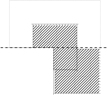
Figure 7: Schematic of corner structure after $2^{k+1}-2$ stages in the third quadrant and $2^{k}$ stages in the upper half.

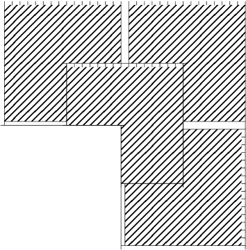
Figure 8: Schematic of corner structure after $2^{k+1}-1$ stages.

It is worth remarking that this growth in three quadrants, one of which is a step ahead of the other two, is responsible for the terms of the form

$$2f(i)+f(i+1)$$ (3)

which appear in the recurrences in Theorems 1, 2 and 4.

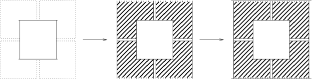
Figure 9: Schematic of evolution of toothpick structure: after $2^{k}$ stages (left-hand figure), after a further $2^{k}-1$ stages (center) and after one more stage (right-hand figure).

3 The toothpick sequences

Similar recurrences hold for the toothpick sequences $t(n)$ and $T(n)$.

Theorem 2

For the toothpick structure discussed in §1, the number of toothpicks added at the $n$th stage is given by $t(0)=0$, $t(1)=1$, and, for $k\geq 1$,

$$t(2^{k}+i)=\begin{cases}2^{k},&\text{if $i=0$};\\ 2t(i)+t(i+1),&\text{if $i=1,\ldots,2^{k}-1$}.\\ \end{cases}$$ (4)

Proof. An inductive argument similar to that used in the proof of Theorem 1 shows that after $2^{k}$ steps, for $k\geq 2$, the toothpick structure is bounded by a $2^{k-1}\times(2^{k-1}-1)$ rectangle, with half-toothpicks protruding horizontally from the four corners, in which all the boundary edges are solid rows of toothpicks, and with no exposed toothpick ends in the interior. (The cases $k=2$ and $3$ can be seen in Fig. 1.) In the induction step, each quadrant grows like a suitably rotated version of the corner structure. (The evolution is depicted schematically in Fig. 9.) The recurrence formula (4) now follows by keeping track of the number of toothpicks that are added as we progress from stage $2^{k}$ to stage $2^{k+1}-1$.    

Corollary 3

For the toothpick sequence $T(n)$, we have $T(0)=0$, and, for $k\geq 0$,

$$T(2^{k}+i)=\begin{cases}\frac{1}{3}(2^{2k+1}+1)&\text{if $i=0$};\\ T(2^{k})+2T(i)+T(i+1)-1,&\text{if $i=1,\ldots,2^{k}-1$}.\\ \end{cases}$$ (5)

Proof. This follows easily from $T(n)=\sum_{i=0}^{n}t(i)$,

$$\sum_{i=2^{k}}^{2^{k+1}-1}t(i)=2^{k}(2^{k+1}-1),$$

and (4). We omit the details.    

$$\begin{array}[]{c|rrrrrrrrrrrrrrrr}k&\lx@intercol\mbox{~{}terms~{}}2^{k},2^{k}+1,\ldots,2^{k+1}-1\hfil\lx@intercol\\ \cline{1-16}\cr 0&0&&&&&&&&&&&&&&&\\ 1&1&&&&&&&&&&&&&&&\\ 2&2&4&&&&&&&&&&&&&&\\ 4&4&4&8&12&&&&&&&&&&&&\\ 8&8&4&8&12&12&16&28&32&&&&&&&&\\ 16&16&4&8&12&12&16&28&32&20&16&28&36&40&60&88&80\\ \ldots&\lx@intercol\ldots\hfil\lx@intercol\end{array}$$

Table 3: Initial terms of toothpick sequence $t(n)$ arranged in triangular form.

A convenient way to visualize the recurrences (2), (4) and (5) is to write the sequences $c(n)$, $t(n)$ and $T(n)$ as triangular arrays, with $1$, $1$, $2$, $4$, $8$, $16$, $32$, $\ldots$ terms in the successive rows. For example, the initial terms of the $t(n)$ sequence are shown in the array in Table 3. The row labeled $8$, for instance, begins with $t(8)=8$, and then, using (4) and referring back to the top of the triangle, continues with the values $t(9)=2t(1)+t(2)=4$, $t(10)=2t(2)+t(3)=8$, $t(11)=2t(3)+t(4)=12$, and so on (a kind of “bootstrap” process).

To see a direct connection between the toothpick sequences and the corner sequences, it is convenient to define $Q(n):=(T(n)-3)/4$ ($n\geq 3$), with $Q(0)=Q(1)=0$. This is the number of toothpicks whose centers are in the interior of the first (or second, third or fourth) quadrants of the toothpick structure. Also let $q(n):=Q(n)-Q(n-1)$ ($n\geq 1$) with $q(0)=0$. The argument used in the proof of Theorem 1 shows that

$$C(n)=2Q(n)+Q(n+1)+2,\quad\mbox{~{}for~{}}n\geq 2\,.$$ (6)

Hence by taking differences we have $q(n)=t(n)/4$,

$$c(n)=2q(n)+q(n+1),\quad\mbox{~{}for~{}}n\geq 3\,,$$ (7)

and

$$c(n)=\frac{1}{2}t(n)+\frac{1}{4}t(n+1),\quad\mbox{~{}for~{}}n\geq 1\,.$$ (8)

4 Rectangles in the toothpick structure

Examination of Figs. 1–3 suggests that, after any finite number of stages, the toothpick structure divides the plane into an unbounded region and a number of squares and rectangles (and no other closed polygonal regions appear). Let $R(n)$ denote the number of squares and rectangles in the toothpick structure after $n$ stages, and let $r(n):=R(n)-R(n-1)$ be the number of squares and rectangles that are added at the $n$th stage. Similarly, let $\rho(n)$ be the number of squares and rectangles that are added to the corner structure at the $n$th stage. The initial values of $\rho(n)$, $r(n)$ and $R(n)$ are shown in Table 4 (these are entries A168131, A160125 and A160124 in [8]).

$$\begin{array}[]{|c|rrrrrrrrrrrrrrrr|}\hline\cr n&0&1&2&3&4&5&6&7&8&9&10&11&12&13&14&15\\ \rho(n)&0&0&1&2&1&1&5&7&3&1&4&5&3&7&18&19\\ r(n)&0&0&0&2&2&0&4&10&6&0&4&8&4&4&20&30\\ R(n)&0&0&0&2&4&4&8&18&24&24&28&36&40&44&64&94\\ \hline\cr\end{array}$$

Table 4: The sequences $\rho(n)$, $r(n)$ and $R(n)$ for $0\leq n\leq 15$.

Then an inductive argument, similar to that used to establish Theorem 1, shows the following.

Theorem 4

All internal regions in the corner and toothpick structures are squares and rectangles. Furthermore, $\rho(0)=\rho(1)=0$, $\rho(2)=1$, $\rho(3)=2$, and, for $k\geq 2$,

$$\rho(2^{k}+i)=\begin{cases}2^{k-1}-1,&\text{if $i=0$};\\ 2\rho(i)+\rho(i+1),&\text{if $i=1,\ldots,2^{k}-3$};\\ 2\rho(i)+\rho(i+1)+1,&\text{if $i=2^{k}-2$}.\\ 2\rho(i)+\rho(i+1)+2,&\text{if $i=2^{k}-1$};\\ \end{cases}$$ (9)

and $r(0)=r(1)=r(2)=0$, $r(3)=2$, and, for $k\geq 2$,

$$r(2^{k}+i)=\begin{cases}2^{k}-2,&\text{if $i=0$};\\ 4\rho(i),&\text{if $i=1,\ldots,2^{k}-2$};\\ 4\rho(i)+2,&\text{if $i=2^{k}-1$}.\\ \end{cases}$$ (10)

We omit the proof.

5 The fractal-like structure

The recursive structure established in the proofs of Theorems 1 and 2 also explains the fractal-like appearance of the toothpick array. After applying one round of the corner recursion to each quadrant and then rescaling, we have the transformation shown schematically in Fig. 10 (an “${\mathbf{F}}$” is used to indicate orientation of the various pieces), and in a specific example in Fig. 11. Note that four of the blocks (the sideways “${\mathbf{F}}$”s) are shifted by a half-toothpick towards the center. Because of this shift the toothpick structure is not strictly self-similar (cf. [3]) and so is not a true fractal. The same is true for all the structures we will meet in this paper: they have a fractal-like growth, but are not strictly self-similar.

Figure 10: Fractal-like transformation recursion, general step.

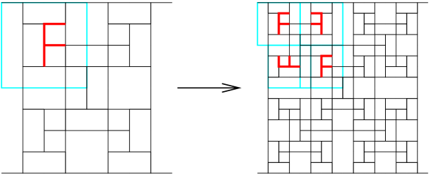
Figure 11: Fractal-like recursion going from stage $8$ to stage $16$.

Figure 12: Plot of toothpick sequence $T(0),\ldots,T(1023)$.

Figure 13: Plot of $(x=\frac{i}{2^{k}},f(x)=\frac{T(n)}{n^{2}})$, $n=2^{k}+i$, $0\leq i<2^{k}$, for $k=14$.

A plot of $T(0),\ldots,T(2^{k}-1)$ for increasing values of $k$ shows that the points lie roughly on a parabola, with irregularities caused by the fractal-like behavior (see for example Fig. 12). Benoît Jubin [6] has investigated $\varlimsup T(n)/n^{2}$ and $\varliminf T(n)/n^{2}$. His numerical results suggest that $\varlimsup T(n)/n^{2}=2/3$, with local maxima at the values $n=2^{k}-1$, and $\varliminf T(n)/n^{2}\approx 0.4513058$ with local minima at the following values of $n$:

$$1,2,5,12,21,44,89,180,362,728,1459,2921,\ldots$$

(see A170927 for further terms). His upper limit can be established from Corollary 3:

Theorem 5

For $n\geq 1$,

$$\frac{T(n)}{n^{2}}\leq\frac{2}{3}+\frac{1}{3n}\,,$$ (11)

with equality if and only if $n=2^{k}-1$ for some $k$. Hence $\varlimsup T(n)/n^{2}=2/3$.

Proof. The result is true for $n\leq 3$, and for $n>3$ for the special values $n=2^{k}-1$, when $T(n)=(2^{k}-1)(2^{k+1}-1)/3$, so

$$\frac{T(n)}{n^{2}}=\frac{2}{3}+\frac{1}{3n}\,,$$

and $n=2^{k}$, when $T(n)=(2^{2k+1}+1)/3$, so

$$\frac{T(n)}{n^{2}}=\frac{2}{3}+\frac{1}{3n^{2}}<\frac{2}{3}+\frac{1}{3n}\,.$$

For the general case we use induction, and assume that (11) holds for all $n\leq 2^{k}$. Let $n=2^{k}+i$, $1\leq i\leq 2^{k}-2$. Then (11) follows from (5) and the induction hypothesis.    

Jubin also observes that there is a continuous function on $[0,1]$ that describes the asymptotic behavior of $T(n)$. This is the function whose graph is the Hausdorff limit of the finite sets $E_{k}$ consisting of the points $(x=\frac{i}{2^{k}},f(x)=\frac{T(n)}{n^{2}})$ for $n=2^{k}+i$, $0\leq i<2^{k}$. This function takes the value $\frac{2}{3}$ at $x=0$ and $x=1$, and has its minimum at around (0.427451, 0.4513058). It is non-differentiable at the dyadic rational points between $0$ and $1$. Figure 13 shows $E_{14}$.

Figure 14: Stages $1$ through $8$ of the evolution of the Ulam-Warburton structure. The numbers of ${\tt ON}$ cells in the successive stages, $U(1),\ldots,U(8)$, are $1,5,9,21,25,37,49,85$.

6 The Ulam-Warburton cellular automaton

As we will see in §10, the toothpick structure can be modeled by a cellular automaton on a planar graph. In this section, we consider a simpler example of the same type, the arrangement of square cells generated by the Ulam-Warburton cellular automaton (Ulam [17], Singmaster [13], Stanley and Chapman [15], Wolfram [22, p. 928]). The cells are the squares in an infinite square grid, and the neighbors of each cell are defined to be the four squares which share an edge with it. (This is the von Neumann neighborhood of the cell, in the notation of [7].) At stage $0$, no cells are ${\tt ON}$. At stage $1$, a single cell is turned ${\tt ON}$. Thereafter, a cell is changed from ${\tt OFF}$ to ${\tt ON}$ at stage $n$ if and only if exactly one of its four neighbors was ${\tt ON}$ at stage $n-1$. Once a cell is ${\tt ON}$ it stays ${\tt ON}$. This is “Rule 686” in the notation of [9], [22].

Let $u(n)$ ($n\geq 0$) denote the number of cells that are changed from ${\tt OFF}$ to ${\tt ON}$ at the $n$th stage, and let $U(n):=\sum_{i=0}^{n}u(i)$ be the total number of ${\tt ON}$ cells after $n$ stages. The initial values of $u(n)$ and $U(n)$ are shown in Table 5. These sequences are respectively entries A147582 and A147562 in [8]. Fig. 14 shows stages $1$ through $8$ of the evolution of the this structure. (As is suggested by Fig. 14 and more particularly by the movie linked to entry A147562, this structure also has a fractal-like growth.)

$$\begin{array}[]{|c|rrrrrrrrrr|}\hline\cr n&0&1&2&3&4&5&6&7&8&9\\ u(n)&0&1&4&4&12&4&12&12&36&4\\ U(n)&0&1&5&9&21&25&37&49&85&89\\ \hline\cr n&10&11&12&13&14&15&16&17&18&19\\ u(n)&12&12&36&12&36&36&108&4&12&12\\ U(n)&101&113&149&161&197&233&341&345&357&369\\ \hline\cr n&20&21&22&23&24&25&26&27&28&29\\ u(n)&36&12&36&36&108&12&36&36&108&36\\ U(n)&405&417&453&489&597&609&645&681&789&825\\ \hline\cr n&30&31&32&33&34&35&36&37&38&39\\ u(n)&108&108&324&4&12&12&36&12&36&36\\ U(n)&933&1041&1365&1369&1381&1393&1429&1441&1477&1513\\ \hline\cr n&40&41&42&43&44&45&46&47&48&49\\ u(n)&108&12&36&36&108&36&108&108&324&12\\ U(n)&1621&1633&1669&1705&1813&1849&1957&2065&2389&2401\\ \hline\cr\end{array}$$

Table 5: The sequences $u(n)$ and $U(n)$ from the Ulam-Warburton cellular automaton, for $0\leq n\leq 49$.

Theorem 6

(i) The number of cells that turn from ${\tt OFF}$ to ${\tt ON}$ at stage $n$ of the Ulam-Warburton cellular automaton satisfies the recurrence $u(0)=1$, $u(1)=1$, and, for $k\geq 0$,

$$u(2^{k}+1+i)=\begin{cases}4,&\text{if $i=0$};\\ 3u(i),&\text{if $i=1,\ldots,2^{k}-1$}.\\ \end{cases}$$ (12)

(ii) There is an explicit formula: $u(0)=0$, $u(1)=1$ and

$$u(n)=4\mathord{\cdot}3^{\operatorname{wt}(n-1)}~{}-~{}1,~{}~{}n\geq 2\,,$$ (13)

where $\operatorname{wt}(n)$, the “binary weight” of $n$, is the number of $1$’s in the binary expansion of $n$ (entry A000120 in [8]).
(iii) The $u(n)$ have generating function

$$x(-\frac{1}{3}+\frac{4}{3}\prod_{k\geq 0}(1+3x^{2^{k}}))\,.$$ (14)

Proof. Part (i) follows by an inductive argument similar to that used in the proofs of Theorems 1 and 2. The appropriate “corner sequence” is A048883, in which the $n$th term is $3^{\operatorname{wt}(n-1)}$ ($n\geq 1$), with partial sums given by A130665. Part (ii) follows from (i) by induction on $n$. Part (iii) follows from the generating function for A048883, which is $\prod_{k\geq 0}(1+3x^{2^{k}})$.    

Remarks.

1. Now the corner sequence has three quadrants that grow in synchronism, so the $2c(i)+c(i+1)$ terms in (2) are replaced by the $3u(i)$ term in (12).

2. Parts (i) and (ii) of the theorem can be found in Singmaster [13] and Stanley and Chapman [15], and part (i) at least was probably known to J. C. Holladay and Ulam. On page 216 of [17], Ulam remarks that for certain structures similar to this one (exactly which ones is left unspecified), J. C. Holladay showed that “at generations whose index number $n$ is of the form $n=2^{k}$, the growth is cut off everywhere except on the ‘stems’, i.e. the straight lines issuing from the original point.” This is certainly consistent with the recurrence (12).

3. Two properties of the Ulam-Warburton structure given in [15] are worth mentioning here. (i) When considered as a subgraph of the infinite square grid, the structure is a tree. This is also true for the toothpick structure—see §10. (ii) Let $n-1=\sum_{i=1}^{w}2^{r_{i}}$ ($r_{1}>r_{2}>\cdots>r_{w}\geq 0$) be the binary expansion of $n-1$. Then a necessary and sufficient condition for the cell at $P=(x,y)\in{\mathbb{Z}}\times{\mathbb{Z}}$ to be turned from ${\tt OFF}$ to ${\tt ON}$ at stage $n>1$ is that $P=\sum_{i=1}^{w}2^{r_{i}}v_{i}$, where $v_{i}\in\{(-1,0),(1,0),(0,-1),(0,1)\}$, subject to $v_{i}\neq-v_{i-1}$ for $i>1$. We have no such characterization of the toothpicks added at the $n$th stage. It is a consequence of this (although it is not mentioned in [15]) that the cells that are turned ${\tt ON}$ at some stage are the cells $(x,y)$ with $x=0$ or $y=0$, and the cells with $xy\neq 0$ for which the highest power of $2$ dividing $x$ is different from the highest power of $2$ dividing $y$. Again we know of no analog for the toothpick structure.

7 Leftist toothpicks

Stimulated by Theorem 6, we set out to look for analogues of (13) and 14 for the toothpick sequence $t(u)$. Our first attempt was a failure, but led to an interesting connection with Sierpiński’s triangle.

We define the “leftist toothpick” structure as follows. We start with a single horizontal toothpick at stage $1$, and extend the structure using the toothpick rule of §1, except that if a toothpick is horizontal, a new toothpick can be added only at its left-hand end. Let $l(n)$ ($n\geq 1$) denote the number of toothpicks added at the $n$th stage, with $l(0)=0$, and let $L(n):=\sum_{i=0}^{n}l(i)$ be the total number of toothpicks after $n$ stages. These are respectively entries A151565 and A151566 in [8]. The initial values of $l(n)$ and $L(n)$ are shown in Table 6. Figure 15 shows the first $15$ stages of the evolution (the starting toothpick is the apex of the triangle, at the right).

$$\begin{array}[]{|c|rrrrrrrrrrrrrrrr|}\hline\cr n&0&1&2&3&4&5&6&7&8&9&10&11&12&13&14&15\\ l(n)&0&1&1&2&2&2&2&4&4&2&2&4&4&4&4&8\\ L(n)&0&1&2&4&6&8&10&14&18&20&22&26&30&34&38&46\\ \hline\cr\end{array}$$

Table 6: The leftist toothpick sequences $l(n)$ and $L(n)$ for $0\leq n\leq 15$.

Figure 15: Stages $1$ through $15$ of the evolution of the leftist toothpick structure.

The reason for investigating this structure is that, at least for the early stages, the part of the toothpick structure of §1 in the $90^{\circ}$ sector $x-2\leq y\leq 2-x$ is essentially equal to the leftist structure. This breaks down, however, at stage $14$. Nevertheless, the leftist structure has some interest. For if we rotate the structure anticlockwise by $90^{\circ}$ and erase all the horizontal toothpicks, we obtain a triangle in which the vertical toothpicks correspond exactly to the positions of the $1$s in Sierpiński’s triangle (i.e., Pascal’s triangle read modulo $2$ [4], [10], [12], [22, Chap. 3]), and the gaps between the vertical toothpicks to the $0$s. Once observed, this is easy to prove.

Gould’s sequence, entry A001316 in [8], gives the number of odd entries in row $n$ of Pascal’s triangle, which is $2^{\operatorname{wt}(n)}$, with generating function $\prod_{k\geq 0}(1+2x^{2^{k}})$. Allowing for the different offset, we conclude that the leftist toothpick sequence $l(n)$ is given by $l(2n-1)=l(2n)=2^{\operatorname{wt}(n-1)}$.

8 Generating functions

The following theorem suggests why generating functions of the form (1) arise in connection with recurrences of the form (2), (4).

Theorem 7

Given integers $\alpha,\beta,\gamma,\delta$, let the Taylor series expansion of

$$x(\alpha+\beta x)\prod_{k\geq 1}(1+\gamma x^{2^{k}-1}+\delta x^{2^{k}})$$ (15)

be $a(0)+a(1)x+a(2)x^{2}+\cdots$. Then we have $a(0)=0,a(1)=\alpha,$ and for $n\geq 2$,

$$a(2^{k}+i)=\begin{cases}\alpha\gamma+\beta{\delta}^{k-1}&\text{if $i=0$};\\ \delta a(i)+\gamma a(i+1),&\text{if $i=1,\ldots,2^{k}-2$};\\ \delta a(i)+\gamma a(i+1)-\alpha{\gamma}^{2},&\text{if $i=2^{k}-1$}.\\ \end{cases}$$ (16)

Proof. The generating function is

$$x(\alpha+\beta x)(1+\gamma x+\delta x^{2})(1+\gamma x^{3}+\delta x^{4})(1+\gamma x^{7}+\delta x^{8})\cdots.$$

Consider the coefficient of $x^{10}$, say. The only way to build up $x^{10}$ is to combine the term $\delta x^{8}$ with $a(2)x^{2}$, or the term $\gamma x^{7}$ with $a(3)x^{3}$. Hence $a(2^{3}+2)=\delta a(2)+\gamma a(3)$. Similar arguments holds for the general case, although adjustments are needed when $i=0$ or $2^{k}-1$. We omit the details.    

An analogous result holds if the product in (15) starts at $k=0$.

Notice the resemblance between Equations (2), (4) and (16). In particular, we have:

Theorem 8

The generating function for the corner sequence $c(n)$ is

$${\mathcal{C}}(x):=x(1+x)\prod_{k\geq 1}(1+x^{2^{k}-1}+2x^{2^{k}})\,.$$ (17)

The generating function for the toothpick sequence $t(n)$ is

$${\mathcal{T}}(x) :=~{}\frac{x}{1+2x}\{1+4x(1+x)\prod_{k\geq 1}(1+x^{2^{k}-1}+2x^{2^{k}})\}$$

$$=~{}\frac{x}{1+2x}\{1+2x\prod_{k\geq 0}(1+x^{2^{k}-1}+2x^{2^{k}})\}\,,$$ (18)

and therefore the generating function for the toothpick sequence $T(n)$ is

$$\frac{x}{(1-x)(1+2x)}\{1+2x\prod_{k\geq 0}(1+x^{2^{k}-1}+2x^{2^{k}})\}\,.$$ (19)

Proof. For the first assertion, we set $\alpha=\beta=\gamma=1$, $\delta=2$ in Theorem 7 and use (2). For the second assertion, we note that (7) implies that the generating functions for $c(n)$ and $q(n)$ are related by

$${\mathcal{C}}(x)=x+x^{2}+(2+\frac{1}{x}){\mathcal{Q}}(x)\,,$$ (20)

and by definition we have

$${\mathcal{T}}(x)=x+2x^{2}+{\mathcal{Q}}(x)\,.$$ (21)

Eliminating ${\mathcal{Q}}(x)$, we obtain (8).    

Remark.

Equation (19) was conjectured by Gary W. Adamson [1]. Consider the sequence $1,1,2,1,3,4,4,1,3,4,5,\ldots$ with generating function

$$\prod_{k\geq 1}(1+x^{2^{k}-1}+2x^{2^{k}})$$

(entry A151550 in [8]). Adamson discovered that if this sequence is convolved with the sequence $1,2,2,2,2,2,\ldots$, the result appeared to coincide with the corner sequence $C(n)$. When expressed in terms of generating functions, his conjecture is essentially equivalent to (19).

9 Explicit formulas

A second comment in [8], this time from Hagen von Eitzen, was instrumental in the discovery of explicit formulas for many of these sequences. Von Eitzen [18] contributed the sequence $2,3,3,3,5,6,4,3,5,6,6,\ldots$ with generating function $\prod_{k\geq 0}(1+x^{2^{k}-1}+x^{2^{k}})$ to [8] (it is entry A160573) and provided an elegant explicit formula for the $n$th term:

$$\sum_{m\geq 0}\binom{\operatorname{wt}(n+m)}{m}\,.$$ (22)

This can be generalized. For this it is convenient to omit the initial linear factors from (1) but to start the product at $k=0$.

Theorem 9

Let the Taylor series expansion of

$$\prod_{k\geq 0}(1+\gamma x^{2^{k}-1}+\delta x^{2^{k}})$$ (23)

be $a(0)+a(1)x+a(2)x^{2}+\cdots$. Then

$$a(n)=\sum_{m\geq 0}{\gamma}^{m}{\delta}^{\operatorname{wt}(n+m)-m}\binom{\operatorname{wt}(n+m)}{m}\,.$$ (24)

Proof. (Based on von Eitzen’s proof of (22).) First, observe that

$$\prod_{k\geq 0}(1+\delta x^{2^{k}})=\sum_{n=0}^{\infty}{\delta}^{\operatorname{wt}(n)}x^{n}\,,$$ (25)

since when getting a term $x^{n}$, we pick up a factor of $\delta$ for every $1$ in the binary expansion of $n$. When we expand

$$\prod_{k\geq 0}(1+\gamma x^{2^{k}-1}+\delta x^{2^{k}})\,,$$ (26)

instead of the product in (25), each time we replace a term $\delta x^{2^{k}}$ by $\gamma x^{2^{k-1}}$, we lose a factor of $x$ in the product, but we gain because there may be several ways to choose the factors in which to do the replacement. Suppose we do this replacement in $m$ of the terms in (26). Then we must increase $n$ to $n+m$, we gain by a factor of $\binom{\operatorname{wt}(n+m)}{m}$, but we have to replace $m$ factors of $\delta$ by $\gamma$s, for a net contribution of ${\gamma}^{m}{\delta}^{\operatorname{wt}(n+m)-m}\binom{\operatorname{wt}(n+m)}{m}$ to the sum.    

Remark.

Note that there are only finitely many nonzero terms in the summations (22) and (24). For large $n$ the number of nonzero terms is roughly $\log_{2}n$. More precisely, the number of nonzero terms for any $n$ is given by entry A100661 in [8].

We can use Theorem 9 to obtain an explicit formula for the toothpick sequence $t(n)$.

Theorem 10

$$t(2^{k}+1+i)=\begin{cases}2\sum_{m\geq 0}{2}^{\operatorname{wt}(i+m)-m}\binom{\operatorname{wt}(i+m)}{m},&\text{if $0\leq i\leq 2^{k}-2$};\\ 2^{k+1},&\text{if $i=2^{k}-1$}.\\ \end{cases}$$ (27)

Proof. This theorem is an instance where our decision to start enumerations at $n=0$ rather than $n=1$ (as discussed in Remark $1$ in §1) causes complications. The result would be more elegant if we had made the other choice. So, just for this proof, let us define $\hat{t}(n)=t(n+1)$ for $n\geq 0$. Then from Theorem 2, $\hat{t}(n)$ satisfies the recurrence

$$\hat{t}(2^{k}+i)=\begin{cases}2\hat{t}(i)+\hat{t}(i+1),&\text{if $i=0,\ldots,2^{k}-2$};\\ 2^{k+1},&\text{if $i=2^{k}-1$}.\\ \end{cases}$$ (28)

$$\begin{array}[]{c|rrrrrrrrrrrrrrrr}k&\lx@intercol\mbox{~{}terms~{}}2^{k},2^{k}+1,\ldots,2^{k+1}-1\hfil\lx@intercol\\ \cline{1-16}\cr 0&1&&&&&&&&&&&&&&&\\ 1&2&&&&&&&&&&&&&&&\\ 2&4&4&&&&&&&&&&&&&&\\ 4&4&8&12&8&&&&&&&&&&&&\\ 8&4&8&12&12&16&28&32&16&&&&&&&&\\ 16&4&8&12&12&16&28&32&20&16&28&36&40&60&88&80&32\\ \ldots&\lx@intercol\ldots\hfil\lx@intercol\end{array}$$

Table 7: Initial terms of sequence $\hat{t}(n)$ arranged in triangular form.

The initial terms of the $\hat{t}(n)$ sequence are shown in triangular array form in Table 7. The initial $2^{k}-1$ terms of the $k$th row are the initial $2^{k}-1$ terms of the next row, so the rows converge to a sequence

$$4,8,12,12,16,28,32,20,16,28,36,\ldots$$

that we will denote by $F(n)$, $n\geq 0$ (this is entry A147646 in [8]). It follows from the definition that $F(n)$ is defined by the recurrence $F(0)=4$, $F(1)=8$, $F(2)=F(3)=12$, and for $n\geq 4$,

$$F(2^{k}+i)=\begin{cases}2F(i)+F(i+1),&\text{if $0\leq i\leq 2^{k}-3$};\\ 2F(i)+F(i+1)-4,&\text{if $i=2^{k}-2$};\\ 2^{k+2}+4,&\text{if $i=2^{k}-1$}.\\ \end{cases}$$ (29)

Also, for $0\leq i\leq 2^{k}-2$,

$$\hat{t}(2^{k}+i)=F(i)\,.$$ (30)

Comparing (29) with Theorem 7, we see (taking $\alpha=\beta=4$, $\gamma=1$, $\delta=2$ in that theorem) that $F(n)$ has generating function

$$4(1+x)\prod_{k\geq 1}(1+x^{2^{k}-1}+2x^{2^{k}})=2\prod_{k\geq 0}(1+x^{2^{k}-1}+2x^{2^{k}})\,.$$ (31)

It follows from Theorem 9 that

$$F(i)=2\sum_{m\geq 0}{2}^{\operatorname{wt}(i+m)-m}\binom{\operatorname{wt}(i+m)}{m}\,.$$ (32)

Then (30) and (32) imply (27).    

10 Cellular automata defined on graphs

Cellular automata defined on graphs were introduced by von Neumann and Ulam in 1949 [16], and the toothpick structure (§1), the corner toothpick structure (§2), the leftist structure (§7), the Ulam-Warburton cellular automaton (§6), etc., can all be described in this language. Let $G$ be an infinite directed (or undirected) graph with finite in-degree and out-degree (or degree) at each node. Nodes are either in the ${\tt OFF}$ state or the ${\tt ON}$ state, and we just need to give a rule for deciding when the nodes change state.

For the toothpick structure, the nodes of $G$ are the vertices $(x,y)\in{\mathbb{Z}}\times{\mathbb{Z}}$ of the square grid. There are two kinds of nodes: “even” nodes, with $x+y$ even, which have edges directed to nodes $(x,y\pm 1)$, and “odd” nodes, with $x+y$ odd, which have edges directed to nodes $(x\pm 1,y)$. Initially all nodes are ${\tt OFF}$, at stage $1$ we turn ${\tt ON}$ node $(0,0)$, and thereafter a node turns ${\tt ON}$ if it has an incoming edge from exactly one ${\tt ON}$ node. This is easily seen to be equivalent to the toothpick structure, with the even (resp. odd) nodes representing the midpoints of vertical (resp. horizontal) toothpicks. The induced subgraph of $G$ joining the ${\tt ON}$ nodes is a directed tree (and remains a tree if the arrows on the edges are removed).

For the Ulam-Warburton cellular automaton, of course, $G$ is the undirected graph with vertices $(x,y)\in{\mathbb{Z}}\times{\mathbb{Z}}$, with each node connected to its four neighbors (or, in the case of the cellular automaton analyzed in §14, its eight neighbors). As already mentioned in §6, the induced subgraph joining the ${\tt ON}$ nodes is also a tree.

For the natural generalization of the Ulam-Warburton cellular automaton to higher dimensions, with $G={{\mathbb{Z}}}^{d}$, $g\geq 1$, and each node adjacent to its $2d$ neighbors, there is an analog of Theorem 6. The number of cells that turn from ${\tt OFF}$ to $ON$ at stage $n$ is given by $u(0)=0$, $u(1)=1$, and, for $n\geq 2$,

$$u(n)=2d\,(2d-1)^{\operatorname{wt}(n-1)-1}$$ (33)

(Stanley and Chapman [15]; see also entries A151779, A151781 in [8]). On the other hand, for the face-centered cubic lattice graph, where each node has $12$ neighbors, there is no obvious formula (see A151776, A151777).

The number of possibilities is endless: see [14] and [22] for further examples.

Figure 16: Stages $1$ through $4$ of the evolution of the T-toothpick structure.

11 T-shaped toothpicks

One may consider “toothpicks” of many other shapes. Here we consider just one example: we define a “T-toothpick” to consist of three line segments of length $1$, forming a “T”. Using an obvious terminology, we will speak of the “crossbar” (which has length $2$) and the “stem” (of length $1$) of the T, and refer to the midpoint of the crossbar as the “midpoint.” A T-toothpick has three endpoints, and an endpoint is said to be “exposed” if it is not the midpoint or endpoint of any other T-toothpick.

We start at stage $1$ with a single T-toothpick in the plane, with its stem vertical and pointing downwards. Thereafter, at stage $n$ we place a T-toothpick at every exposed endpoint, with the midpoint of the new T-toothpick touching the exposed endpoint and with its stem pointing away from the existing T-toothpick. Figure 16 shows the first four stages of the evolution. Let $\tau(n)$ denote the number of T-toothpicks added to the structure at the $n$th stage (this is A160173).

Theorem 11

We have $\tau(0)=0$, $\tau(1)=1$, $\tau(2)=3$, and, for $n\geq 3$,

$$\tau(n)=\frac{2}{3}\{3^{\operatorname{wt}(n-1)}+3^{\operatorname{wt}(n-2)}\}+1\,.$$ (34)

Proof. This is easily established from Theorem 6 by observing that the structures in the four quadrants defined by the the initial T are essentially equivalent to copies of the Ulam-Warburton structure. The copies in the first and second quadrants are one stage behind those in the third and fourth quadrants.    

The analogous structure using Y-shaped toothpicks has resisted our attempts to analyze it—see A160120 in [8].

12 The “Maltese cross” or Holladay-Ulam structure

On page 217 of [17], Ulam discusses another structure that he and J. C. Holladay had studied. To construct this, one first builds the infinite Ulam-Warburton structure described in §6, and then replaces each ${\tt ON}$ cell by a Maltese cross consisting of a central ${\tt ON}$ cell surrounded by four other ${\tt ON}$ cells. Now label the cells of the new infinite structure, starting by labeling the central square $1$, then the four adjacent cells $2$, and so on, always moving outwards from the center. Figure 17 shows the cells with labels $1$ through $5$.

Figure 17: Stages $1$ through $5$ of the evolution of the Maltese cross structure.

Holladay and Ulam then give a set of rules for a cellular automaton that will build up this structure, starting with the cell labeled $1$. We found their rules (stated on pages 216 and 222) somewhat hard to understand, so it may be helpful to the reader if we give our version of them here.

For a candidate cell to be turned ${\tt ON}$ it is necessary (though not sufficient) that it share exactly one edge with an ${\tt ON}$ cell of the previous generation. The two vertices of the candidate cell that touch that edge we will call its inner vertices, and the other two vertices we call its outer vertices.

The rules are as follows. Cells are in one of three states, ${\tt OFF}$, ${\tt ON}$ or ${\tt DEAD}$. Once a cell is ${\tt ON}$ or ${\tt DEAD}$ it remains in that state. Initially all cells are ${\tt OFF}$, and at stage $1$ a single cell is turned ${\tt ON}$.

At stage $n$, consider ${\tt OFF}$ cells $X$ (the “candidates”) that share at least one edge with an ${\tt ON}$ cell of the previous generation. If a candidate $X$ is edge-adjacent to two ${\tt ON}$ cells, $X$ is declared ${\tt DEAD}$. If two candidates $X$ and $X^{\prime}$ share an outer vertex, both $X$ and $X^{\prime}$ are declared ${\tt DEAD}$. If a candidate $X$ is edge-adjacent to a ${\tt DEAD}$ cell, then $X$ is declared ${\tt DEAD}$, except that when $n\equiv 2$ (mod $3$), this rule obtains only if $X$ is edge-adjacent to a cell that was declared ${\tt DEAD}$ at the previous generation. If a candidate is not excluded by these conditions, it is turned ${\tt ON}$.

Figure 18 is an annotated picture showing the first eight stages of the evolution of this structure in the first quadrant, with letters identifying the first few ${\tt DEAD}$ cells. The letters ‘a’ and ‘d’ indicate candidate cells that are ${\tt DEAD}$ because they are edge-adjacent to two ${\tt ON}$ cells, and ‘b’ and ‘e’ indicate candidate cells that are ${\tt DEAD}$ because they are edge-adjacent to a ${\tt DEAD}$ cell and $n$ is not congruent to $2$ (mod $3$). The ‘5’ cells not on the main axes are ${\tt ON}$ because $5\equiv 2$ (mod $3$). The two ‘c’ cells are ${\tt DEAD}$ because they would share a common outer vertex; and so on.

Figure 18: Annotated version of stages $1$ through $8$ of the Maltese cross structure in the first quadrant.

Of course, the original definition of this structure makes it easy to give a formula for the number of cells, $m(n)$, say, that are added at the $n$th stage. From (13) we have $m(0)=0$, $m(1)=1$, $m(2)=4$, and, for $t\geq 1$,

$$m(3t)=m(3t+1)=4\mathord{\cdot}3^{\operatorname{wt}(t)-1},~{}m(3t+2)=4\mathord{\cdot}3^{\operatorname{wt}(t)}.$$ (35)

(This is entry A151906 in [8].)

We conclude this section by listing some related cellular automata studied by Ulam and his colleagues Holladay and Schrandt in [11] and [17]. Since we have not even found recurrences for them, we will give no details.

Reference [11] mentions a cellular automaton which is intermediate in complexity between the Ulam-Warburton structure and the Maltese cross structure discussed above. This Schrandt-Ulam cellular automaton is described in entries A170896 and A170897 in [8]; another version is given in A151895, A151896.

Analogous structures based on triangles or hexagons rather than squares are described in Examples $3$ through $6$ of [17] (see also Wolfram [22, p. 371]), and in entries A151723, A151724, A161644, A161645 of [8]. We invite the reader to find recurrences or generating functions for any of them.

13 Rule 942

On page 928 of [22], Wolfram considers (among other examples) what happens if the rule for the Ulam-Warburton cellular automaton is modified so that a cell turns ${\tt ON}$ if and only if either exactly one or all four of its four neighbors is ${\tt ON}$ (this is “Rule 942” in the notation of [9], [22]).

Let $w(n)$ denote the number of cells that are changed from ${\tt OFF}$ to ${\tt ON}$ at stage $n$. Since the four-neighbor part of the rule is invoked only after an ${\tt OFF}$ cell is completely surrounded by ${\tt ON}$ cells, $w(n)\geq u(n)$ for all $n$. In fact, $w^{\prime}(n):=w(n)-u(n)$ is always a multiple of $4$, and $w(n)=u(n)$ except when $n\equiv 1~{}(\mbox{mod~{}}n)$. Table 8 shows the initial values of $w(n)$, $u(n)$, $w^{\prime}(n)$ and $\delta(n):=\frac{1}{4}(w(4n+1)-u(4n+1))$ (cf. A169648 and A169689 in [8]).

$$\begin{array}[]{|c|rrrrrrrrrrrrrrrr|}\hline\cr n&0&1&2&3&4&5&6&7&8&9&10&11&12&12&14&15\\ w(n)&0&1&4&4&12&8&12&12&36&28&12&12&36&28&36&36\\ u(n)&0&1&4&4&12&4&12&12&36&4&12&12&36&12&36&36\\ w^{\prime}(n)&0&0&0&0&0&4&0&0&0&24&0&0&0&16&0&0\\ \delta(n)&0&1&6&4&24&4&20&12&84&4&20&12&76&12&60&36\\ \hline\cr\end{array}$$

Table 8: The sequences $w(n)$, $u(n)$, $w^{\prime}(n0:=w(n)-u(n)$, $\delta(n)$ for $0\leq n\leq 15$.

There is a simple explicit formula for $\delta(n)$ and hence, via (13), for $w(n)$.

Theorem 12

We have $\delta(0)=0$, $\delta(1)=1$, $\delta(2)=6$. For $n\geq 3$, let $n=2^{k}+j$ with $1\leq j\leq 2^{k}$, where $j=2^{m}(2l+1)$ (say). Then

$$\delta(n)=4(3^{m+1}-2^{m+1})3^{\operatorname{wt}(l)}\,,$$ (36)

except that if $j=2^{k}$ then

$$\delta(n)=4\mathord{\cdot}3^{k+1}-3\mathord{\cdot}2^{k+1}\,.$$ (37)

We omit the proof, which is similar to those of Theorems 1 and 2.

14 Square grid with eight neighbors

Our final example is also based on the Ulam-Warburton cellular automaton, except that now we take the neighbors of a cell to consist of the eight cells surrounding it. (This is the Moore neighborhood of the cell, in the notation of [7].) Otherwise the rules are the same as in §6: a cell turns ${\tt ON}$ if exactly one of its eight neighbors is ${\tt ON}$.

Let $v(n)$ ($n\geq 0$) denote the number of cells that are changed from ${\tt OFF}$ to ${\tt ON}$ at the $n$th stage of the evolution, and let $V(n):=\sum_{i=0}^{n}v(i)$ be the total number of ${\tt ON}$ cells after $n$ stages. The initial values of $v(n)$ and $V(n)$ are shown in Table 9 below. These sequences are respectively entries A151726 and A151725 in [8]. Figure 19 shows stages $1$ through $8$ of the evolution of the this structure.

Figure 19: Stages $1$ through $8$ of the evolution of the eight-neighbor structure. The numbers of ${\tt ON}$ cells in the successive stages, $V(1),\ldots,V(8)$, are $1,9,13,33,37,57,77,121$.

Since each cell now has two kinds of neighbors, it is perhaps not surprising that this problem is more difficult to analyze than the Ulam-Warburton structure. In order to understand the growth, it is convenient to define two versions of “corner sequences,” analogous to that introduced in §2.

So that we can refer to individual cells, we will label each square cell by the grid point at its upper left corner. That is, we define cell $(i,j)$ to consist of the square $\{(x,y)\in{\mathbb{R}}\times{\mathbb{R}}\mid i\leq x\leq i+1,~{}j-1\leq y\leq j\}$.

For the first corner sequence, we exclude the third quadrant of the plane, and at stage $1$ we turn ${\tt ON}$ the cell immediately to the right of that quadrant (see Fig. 20). More precisely, at stage $1$, we turn ${\tt ON}$ the cell $(0,0)$, and thereafter extend the structure using the eight-neighbor rule, with the proviso that after the first stage, no ${\tt ON}$ cell may be adjacent to any of the third-quarter cells—meaning the cells $(i,j)\in{\mathbb{Z}}\times{\mathbb{Z}}$ with $i\leq-1,j\leq 0$.

The second corner sequence is similar to the first, except that at stage $1$ we turn ${\tt ON}$ the cell $(0,1)$, just up and to the right of the excluded quadrant (Fig. 21).

Let $v_{1}(n)$ (resp. $v_{2}(n)$) denote the number of cells that are changed from ${\tt OFF}$ to ${\tt ON}$ at the $n$th stage of the evolution of the first (resp. second) corner sequence. The initial values of $v_{1}(n)$ and $v_{2}(n)$ are also shown in Table 9. These sequences are respectively entries A151747 and A151728 in [8]. Figures 20 and 21 shows stages $1$ through $5$ of the evolution of the two corner sequences.

$$\begin{array}[]{|c|rrrrrrrrrr|}\hline\cr n&0&1&2&3&4&5&6&7&8&9\\ v(n)&0&1&8&4&20&4&20&20&44&4\\ V(n)&0&1&9&13&33&37&57&77&121&125\\ v_{1}(n)&0&1&3&5&8&9&11&17&21&15\\ v_{2}(n)&0&1&5&5&11&7&15&19&23&7\\ \hline\cr n&10&11&12&13&14&15&16&17&18&19\\ v(n)&20&20&44&28&60&76&92&4&20&20\\ V(n)&145&165&209&237&297&373&465&469&489&509\\ v_{1}(n)&11&18&25&29&39&54&53&27&11&18\\ v_{2}(n)&15&21&29&29&49&59&47&7&15&21\\ \hline\cr n&20&21&22&23&24&25&26&27&28&29\\ v(n)&44&28&60&76&92&28&60&84&116&116\\ V(n)&553&581&641&717&809&837&897&981&1097&1213\\ v_{1}(n)&25&29&39&55&57&41&40&61&79&97\\ v_{2}(n)&29&29&49&61&53&29&51&71&87&107\\ \hline\cr\end{array}$$

Table 9: The $8$-neighbor sequences $v(n)$ and $V(n)$, and the two “corner” sequences $v_{1}(n)$, $v_{2}(n)$, for $0\leq n\leq 23$.

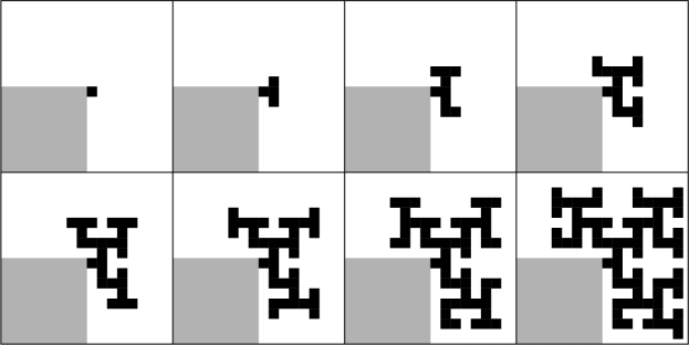
Figure 20: Stages $1$ through $8$ of the evolution of the first corner sequence $v_{1}(n)$.

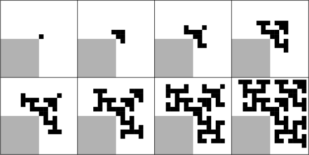
Figure 21: Stages $1$ through $8$ of the evolution of the second corner sequence $v_{2}(n)$.

The following theorem gives recurrences for all three of these sequences.

Theorem 13

The eight-neighbor sequences $v_{1}(n)$, $v_{2}(n)$ and $v(n)$ satisfy the following recurrences:

$v_{1}(0)=0$, $v_{1}(1)=1$, $v_{1}(2)=3$, $v_{1}(3)=5$, and, for $k\geq 2$,

$$v_{1}(2^{k}+i)=\begin{cases}(3k+1)\,2^{k-2}+1,&\text{if $i=0$};\\ 3\mathord{\cdot}2^{k-1}+3,&\text{if $i=1$};\\ 2\,v_{1}(i)+v_{1}(i+1),&\text{if $i=2,\ldots,2^{k}-2$};\\ 2\,v_{1}(i)+v_{1}(i+1)-1,&\text{if $i=2^{k}-1$};\\ \end{cases}$$ (38)

$v_{2}(0)=0$, $v_{2}(1)=1$, and, for $k\geq 1$,

$$v_{2}(2^{k}+i)=\begin{cases}3\mathord{\cdot}2^{k}-1,&\text{if $i=0$};\\ v_{2}(i)+2\,v_{1}(i+1),&\text{if $i=1,\ldots,2^{k}-2$};\\ v_{2}(i)+2\,v_{1}(i+1)-2,&\text{if $i=2^{k}-1$};\\ \end{cases}$$ (39)

$v(0)=0$, $v(1)=1$, and, for $k\geq 1$,

$$v(2^{k}+i)=\begin{cases}6\mathord{\cdot}2^{k}-4,&\text{if $i=0$};\\ 4\,v_{2}(i),&\text{if $i=1,\ldots,2^{k}-1$}.\\ \end{cases}$$ (40)

Again we omit the proof. We have not found generating functions or explicit formulas for any of these sequences.

15 Acknowledgments

We thank Benoît Jubin for telling us about his investigations into the asymptotic behavior of $T(n)$ that were discussed in §5, and Gary Adamson and Hagen von Eitzen for their contributions to [8] which were mentioned in §8 and §9. We also thank Maximilian Hasler, John Layman and Richard Mathar, who have made many contributions to [8] (especially new sequences or extensions of existing sequences) related to the subject of this paper. Finally, we thank Laurinda Alcorn for locating a copy of [11].

References

- [1] G. W. Adamson, Comment on entry A151550 in [8], May 25, 2009.
- [2] E. R. Berlekamp, J. H. Conway and R. K. Guy, Winning Ways for Your Mathematical Plays, A. K. Peters, Wellesley, MA, 2nd. ed., 4 vols., 2001–2004.
- [3] K. Falconer, Fractal Geometry, Wiley, NY, 1990.
- [4] S. R. Finch, Mathematical Constants, Cambridge, 2003, p. 145.
- [5] H. Gingold, H. W. Gould and M. E. Mays, Power product expansions, Until. Math., 34 (1988), 143–161.
- [6] B. Jubin, Personal communication, January, 2010.
- [7] M. Mitchell, Computation in cellular automata: a selected review, pp. 95–140 of T. Gramß et al., Nonstandard Computation, Wiley-VCH, Weinheim, 1996.
- [8] The OEIS Foundation Inc., The On-Line Encyclopedia of Integer Sequences, http://oeis.org, 2010.
- [9] N. H. Packard and S. Wolfram, Two-dimensional cellular automata, J. Statistical Physics, 38 (1985), 901–946.
- [10] H.-O. Peitgen, H. Jürgens and D. Saupe, Chaos and Fractals, Springer-Verlag, NY, 1992, pp. 408–409.
- [11] R. G. Schrandt and S. M. Ulam, On recursively defined geometric objects and patterns of growth, Los Alamos Scientific Laboratory, Los Alamos, NM, Report LA–3762, Aug 16 1967; published in A. W. Burks, editor, Essays on Cellular Automata, Univ. Ill. Press, 1970, pp. 238ff. Available on-line from http://library.lanl.gov/cgi-bin/getfile?00359037.pdf.
- [12] M. Schroeder, Fractals, Choas, Power Laws, W. H. Freeman, NY, 1991, Chap. 17.
- [13] D. Singmaster, On the cellular automaton of Ulam and Warburton, M500 Magazine of The Open University, #195 (December 2003), 2–7.
- [14] N. J. A. Sloane, Catalog of Toothpick and Cellular Automata Sequences in the OEIS, published electronically at http://www.research.att.com/njas/sequences/toothlist.html, 2010.
- [15] R. P. Stanley (proposer) and R. J. Chapman (solver), A tree in the integer lattice, Problem 10360, Amer. Math. Monthly, 101 (1994), 76; 105 (1998), 769–771.
- [16] S. M. Ulam, Random processes and transformations, in Proc. International Congress Mathematicians, Cambridge, MA, 1950, Amer. Math. Soc., Providence, RI, 1952, Vol. 2, pp. 264–275.
- [17] S. M. Ulam, On some mathematical problems connected with patterns of growth of figures, pp. 215–224 of R. E. Bellman, ed., Mathematical Problems in the Biological Sciences, Proc. Sympos. Applied Math., Vol. 14, Amer. Math. Soc., 1962.
- [18] H. von Eitzen, Entry A160573 in [8], May 20, 2009.
- [19] E. W. Weisstein, Rule 30, published electronically at http://mathworld.wolfram.com/Rule30.html (From MathWorld–A Wolfram Web Resource).
- [20] S. Wolfram, Statistical mechanics of cellular automata, Rev. Mod. Phys., 55 (1983), 601–644.
- [21] S. Wolfram, The Mathematica® Book, Wolfram Media, Champaign, IL, 3rd. ed., 1996.
- [22] S. Wolfram, A New Kind of Science, Wolfram Media, Champaign, IL, 2002.