A Note on the Smoluchowski-Kramers Approximation for the Langevin Equation with Reflection

Abstract

According to the Smoluchowski-Kramers approximation, the solution of the equation $\mu\ddot{q}^{\mu}_{t}=b(q^{\mu}_{t})-\dot{q}^{\mu}_{t}+\Sigma(q^{\mu}_{t})\dot{W}_{t},q^{\mu}_{0}=q,\dot{q}^{\mu}_{0}=p$ converges to the solution of the equation $\dot{q}_{t}=b(q_{t})+\Sigma(q_{t})\dot{W}_{t},q_{0}=q$ as $\mu\rightarrow 0$. We consider here a similar result for the Langevin process with elastic reflection on the boundary.

Keywords: Smoluchowski-Kramers approximation, reflection, Langevin equation, Skorohod reflection problem.

This is an electronic reprint of the original article published by the World Scientific Publishing Company in Stochastics and Dynamics, Vol. 7, No. 2, June 2007 , 141-153. This reprint differs from the original in pagination and typographic detail.

1 Introduction

The well-known Smoluchowski-Kramers approximation ([9],[8]) implies that the solution of the stochastic differential equation (S.D.E.)

$$\mu\ddot{q}^{\mu}_{t} = b(q^{\mu}_{t})-\dot{q}^{\mu}_{t}+\Sigma(q^{\mu}_{t})\dot{W}_{t}$$ (1)

$$q^{\mu}_{0} = q\in\mathbb{R}^{r}$$

$$\dot{q}^{\mu}_{0} = p\in\mathbb{R}^{r}$$

converges in probability as $\mu\rightarrow 0$ to the solution of the following S.D.E.:

$$\dot{q}_{t} = b(q_{t})+\Sigma(q_{t})\dot{W}_{t}$$ (2)

$$q_{0} = q\in\mathbb{R}^{r},$$

where $b=(b_{1},...,b_{r})^{{}^{\prime}}$ (the transpose of $(b_{1},...,b_{r})$) with $b_{j}:\mathbb{R}^{r}\rightarrow\mathbb{R},j=1,..,r$, $\Sigma=[\sigma_{ij}]_{i,j}^{r}$ with $\sigma_{ij}:\mathbb{R}^{r}\rightarrow\mathbb{R},i,j=1,..,r$ have bounded first derivatives and $W_{t}=(W_{t}^{1},...,W_{t}^{r})^{{}^{\prime}}$ is the standard r-dimensional Wiener process. In other words, one can prove that for any $\delta,T>0$ and $q,p\in\mathbb{R}^{r}$ (see, for example, Lemma 1 in [6]),

$$\lim_{\mu\downarrow 0}P(\max_{0\leq t\leq T}|q^{\mu}_{t}-q_{t}|>\delta)=0.$$ (3)

Equation (1) describes the motion of a particle of mass $\mu$ in a force field $b(q)+\Sigma(q)\dot{W}_{t}$ with a friction proportional to velocity. The Smoluchowski-Kramers approximation justifies the use of equation (2) to describe the motion of a small particle.

It is easy to see now that (1) can be equivalently written as:

$$\dot{q}^{\mu}_{t} = p^{\mu}_{t}$$

$$\mu\dot{p}^{\mu}_{t} = b(q^{\mu}_{t})-p^{\mu}_{t}+\Sigma(q^{\mu}_{t})\dot{W}_{t}$$ (4)

$$q^{\mu}_{0} = q\in\mathbb{R}^{r},\hskip 2.84544pt\dot{q}^{\mu}_{0}=p\in\mathbb{R}^{r}.$$

Let us define $\mathbb{R_{+}}=\{q^{1}\in\mathbb{R}:q^{1}\geq 0\}$ and let the configuration space be $D=\mathbb{R_{+}}\times\mathbb{R}^{r-1}$. In this paper we examine the behavior of the process with elastic reflection on the boundary $\partial D\times\mathbb{R}^{r}=(\partial\mathbb{R_{+}}\times\mathbb{R}^{r-1})\times\mathbb{R}^{r}$ of the phase space $D\times\mathbb{R}^{r}$ that is governed by (4), i.e. of the Langevin process with reflection, as $\mu\rightarrow 0$ when $\Sigma$ is the unit matrix. We will show that the first component (the q component) of the Langevin process with reflection at $q^{1}=0$, that is governed by equation (4), converges in distribution to the diffusion process with reflection on $\partial D$ that is governed by (2). The method is based on properties of the Skorohod reflection problem and in techniques developed in [2] and in [3]. In section 2 we define the Langevin process with reflection for general diffusion matrx $\Sigma$ with inputs that have bounded first derivatives, in section 3 we describe the Skorohod reflection problem and in section 4 we consider the limit $\mu\rightarrow 0$ when the diffusion matrix is the unit matrix. We note here that the limit when $\mu\rightarrow 0$ for a general diffusion matrix as above can be examined similarly.

2 Langevin process with reflection and preliminary results

We begin with the construction of the Langevin process $(q^{\mu}_{t};p^{\mu}_{t})$ in $D\times\mathbb{R}^{r}$ with elastic reflection on the boundary. Let $b=(b_{1},...,b_{r})^{{}^{\prime}}$ with $b_{j}:D\rightarrow\mathbb{R},j=1,..,r$ and $\Sigma=[\sigma_{ij}]$ with $\sigma_{ij}:D\rightarrow\mathbb{R},i,j=1,..,r$ have bounded first derivatives and $\Sigma$ be non-degenerate. Let $(q,p)\in D\times\mathbb{R}^{r}$ be the initial point (we assume that $(q^{1})^{2}+(p^{1})^{2}\neq 0$). Then $(q^{\mu}_{t};p^{\mu}_{t})$ is the right-continuous Markov process in $D\times\mathbb{R}^{r}$ defined as follows. Consider the following system of S.D.E.’s:

$$\dot{q}^{i,\mu}_{t} = p^{i,\mu}_{t}$$

$$\mu\dot{p}^{i,\mu}_{t} = -p^{i,\mu}_{t}+b_{i}(q^{\mu}_{t})+\sum_{j=1}^{r}\sigma_{ij}(q^{\mu}_{t})\dot{W}_{t}^{j}$$ (5)

$$q^{i,\mu}_{0} = q^{i},\hskip 2.84544ptp^{i,\mu}_{0}=p^{i},\hskip 2.84544pti=1,...,r.$$

We define $(q^{\mu}_{t};p^{\mu}_{t})$ to be the solution to (5) for $t\in[0,\tau_{1}^{\mu})$, where $\tau_{1}^{\mu}=\inf\{t>0:q_{t}^{1,\mu}=0\}$. Then define $(q^{\mu}_{t};p^{\mu}_{t})$ for $t\in[\tau_{1}^{\mu},\tau_{2}^{\mu})$, where $\tau_{2}^{\mu}=\inf\{t>\tau_{1}^{\mu}:q_{t}^{\mu}=0\}$, to be the solution of (5) with initial conditions

$$(q_{\tau_{1}^{\mu}}^{\mu};p_{\tau_{1}^{\mu}}^{\mu})=(0,\lim_{t\uparrow\tau_{1}^{\mu}}q_{t}^{2,\mu},...,\lim_{t\uparrow\tau_{1}^{\mu}}q_{t}^{r,\mu};-\lim_{t\uparrow\tau_{1}^{\mu}}p_{t}^{1,\mu},\lim_{t\uparrow\tau_{1}^{\mu}}p_{t}^{2,\mu},...,\lim_{t\uparrow\tau_{1}^{\mu}}p_{t}^{r,\mu}).$$

If $0<\tau_{1}^{\mu}<\tau_{2}^{\mu}<...<\tau_{k}^{\mu}$ and $(q^{\mu}_{t};p^{\mu}_{t})$ for $t\in[0,\tau_{k}^{\mu})$ are already defined, then define $(q^{\mu}_{t};p^{\mu}_{t})$ for $t\in[\tau_{k}^{\mu},\tau_{k+1}^{\mu})$ as solution of (5) with initial conditions

$$(q_{\tau_{k}^{\mu}}^{\mu};p_{\tau_{k}^{\mu}}^{\mu})=(0,\lim_{t\uparrow\tau_{k}^{\mu}}q_{t}^{2,\mu},...,\lim_{t\uparrow\tau_{k}^{\mu}}q_{t}^{r,\mu};-\lim_{t\uparrow\tau_{k}^{\mu}}p_{t}^{1,\mu},\lim_{t\uparrow\tau_{k}^{\mu}}p_{t}^{2,\mu},...,\lim_{t\uparrow\tau_{k}^{\mu}}p_{t}^{r,\mu})$$

(see Figure 1 for an illustration).

This construction defines the process $(q^{\mu}_{t};p^{\mu}_{t})$ in $D\times\mathbb{R}^{r}$ for all $t\geq 0$. This follows from Theorem 2.4, which states that the process that we constructed above does not have infinitely many jumps in any finite time interval $[0,T]$. Therefore we have the following definition:

Definition 2.1. We call the above recursively constructed process, the Langevin process with elastic reflection on the boundary $\partial D\times\mathbb{R}^{r}$. This process has jumps on $\partial D\times\mathbb{R}^{r}$ and is continuous inside $D\times\mathbb{R}^{r}$.

We will refer to the Langevin process with reflection as l.p.r.$(q_{t}^{\mu};p_{t}^{\mu})$. Moreover we will denote by $(q^{\mu,q}_{t};p^{\mu,p}_{t})$ the trajectories of $(q_{t}^{\mu};p_{t}^{\mu})$ with initial position $(q,p)$. For easy of notation we also define $-x=(-x^{1},x^{2},\dots,x^{r})$ and $|x|=(|x^{1}|,x^{2},\dots,x^{r})$ for $x\in\mathbb{R}^{r}$.

Below we see an illustration of the construction above in the $(q^{1}-p^{1})$ phase space.

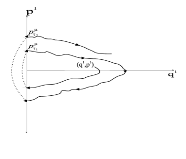
Figure 1: Illustration of the Langevin process with reflection in the $(q^{1}-p^{1})$ phase space

Let us give now another construction of the Langevin process with reflection. Consider the following S.D.E. in $\mathbb{R}^{2r}$:

$$\dot{q}^{1,\mu}_{t} = p^{1,\mu}_{t}$$

$$\mu\dot{q}^{1,\mu}_{t} = -p^{1,\mu}_{t}+\textrm{sgn}(q^{1,\mu}_{t})b_{1}(|q^{\mu}_{t}|)+\sum_{j=1}^{r}\textrm{sgn}(q^{1,\mu}_{t})\sigma_{1j}(|q^{\mu}_{t}|)\dot{W}_{t}^{j}$$

$$q^{1,\mu}_{0} = q^{1},p^{1,\mu}_{0}=p^{1},$$

$$\dot{q}^{i,\mu}_{t} = p^{i,\mu}_{t}$$ (6)

$$\mu\dot{p}^{i,\mu}_{t} = -p^{i,\mu}_{t}+b_{i}(|q^{\mu}_{t}|)+\sum_{j=1}^{r}\sigma_{ij}(|q^{\mu}_{t}|)\dot{W}_{t}^{j}$$

$$q^{i,\mu}_{0} = q^{i},p^{i,\mu}_{0}=p^{i},i=2,...,r,$$

where $\textrm{sgn}(x)$ takes two values, 1 if $x\geq 0$ and -1 if $x<0$.

Lemma 2.2. Equation (6) has a weak solution which is unique in the sense of probability law.

Proof. The existence follows from the Girsanov’s Theorem on the absolute continuous change of measures in the space of trajectories (b and $\Sigma$ are assumed bounded) and the fact that (6) with $b=0$ has a weak solution. The uniqueness follows from Proposition 5.3.10 of [7].

$\Box$

Using the processes $(q^{\mu,q}_{t};p^{\mu,p}_{t})$ and $(q^{\mu,-q}_{t};p^{\mu,-p}_{t})$ we can give another construction of the Langevin process with reflection, as follows. Assume that $q^{1}>0$ and $p^{1}>0$, The graphs of $p^{1,\mu,p^{1}}_{t}$ and $p^{1,\mu,-p^{1}}_{t}$ will be exactly symmetric with respect to zero. The same will be true also for the graphs of $q^{1,\mu,q^{1}}_{t}$ and of $q^{1,\mu,-q^{1}}_{t}$. Let $\tau_{0}^{\mu}=0,\tau_{k}^{\mu}=\inf\{t>\tau_{k-1}^{\mu}:q_{t}^{1,\mu,q^{1}}=0\}$ and $(\widehat{q}^{\mu}_{t};\widehat{p}^{\mu}_{t})$ be a stochastic process, which is defined as follows:

$$(\widehat{q}^{\mu}_{t};\widehat{p}^{\mu}_{t}) = (q^{\mu,q}_{t};p^{\mu,p}_{t})\textrm{ for }\tau_{2k}^{\mu}\leq t\leq\tau_{2k+1}^{\mu,-}$$

$$(\widehat{q}^{\mu}_{t};\widehat{p}^{\mu}_{t}) = (q^{\mu,-q}_{t};p^{\mu,-p}_{t})\textrm{ for }\tau_{2k+1}^{\mu}\leq t\leq\tau_{2k+2}^{\mu,-},k=0,1,2,...$$ (7)

Process $(\widehat{q}^{\mu}_{t};\widehat{p}^{\mu}_{t})$ is a process with reflection and it can be seen that $(\widehat{q}^{\mu}_{t};\widehat{p}^{\mu}_{t})$, which is the same as $(|q^{1,\mu}_{t}|,q^{2,\mu}_{t},\cdots,q^{r,\mu}_{t};\frac{d}{dt}|q^{1,\mu}_{t}|,\dot{q}^{2,\mu}_{t},\cdots,\dot{q}^{r,\mu}_{t})$, and l.p.r.$(q^{\mu}_{t};p^{\mu}_{t})$ coincide.

In the figures below we give an illustration of the construction of $(\widehat{q}^{1,\mu}_{t};\widehat{p}^{1,\mu}_{t})$. The first figure illustrates with thick continuous and dotted lines $\widehat{q}^{1,\mu}_{t}$ versus $t$. The continuous line is $q^{1,\mu,q^{1}}_{t}$ versus $t$ and the dotted is $q^{1,\mu,-q^{1}}_{t}$ versus $t$. The second figure illustrates with thick continuous and dotted lines $\widehat{p}^{1,\mu}_{t}$ versus $t$. The continuous line is $p^{1,\mu,p^{1}}_{t}$ versus $t$ and the dotted is $p^{1,\mu,-p^{1}}_{t}$ versus $t$.

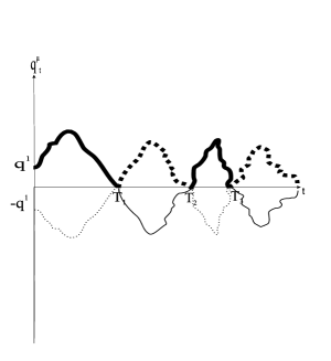
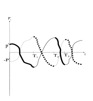
Figure 2: Illustration of the process with reflection

Lemma 2.3. Let $T>0$. The Markov process $(q^{\mu}_{t};p^{\mu}_{t})$ starting at a point $(q,p)$ different from the origin $\textrm{O}=(0,...,0;0,...,0)$, that satisfies system (6), does not reach the origin O in finite time T, i.e.

$$P(\exists t\leq T\hskip 2.84544pts.t.\hskip 2.84544pt(q^{\mu}_{t};p^{\mu}_{t})=\textrm{O})=0.$$

Proof. We easily see that it is actually enough to consider only $(q^{1,\mu}_{t};p^{1,\mu}_{t})$. Let $\delta\ll 1$ be a small number. Define the rectangle $\Delta=\{(q,p)\in\mathbb{R}\times\mathbb{R}:|q|\leq\frac{\delta^{2}}{2},|p|\leq\frac{\delta}{2}\}$ and suppose that the trajectory starts from some point outside the rectangle $\Delta$, say from $(q,0)\in\mathbb{R}^{2}\setminus\Delta$. Let also $\chi_{\Delta}(x)$ denote the indicator function of the set $\Delta$. Then $E^{(q,0)}\int_{0}^{T}\chi_{\Delta}(q_{s}^{1},p_{s}^{1})ds$ is the expected value of the time ,during time $[0,T]$, that the process $(q_{t}^{1},p_{t}^{1})$ with initial point $(q,0)$ spends inside the rectangle $\Delta$. If $b=0$ and $\Sigma$ is a matrix with constant entries, $(q^{1}_{t},p^{1}_{t})$ is a Gaussian process. One can write down its density explicitly (see equation (6)), which we denote by $\rho(\cdot)$, and obtain the bound

$$E^{(q,0)}\int_{0}^{T}\chi_{\Delta}(q_{s}^{1},p_{s}^{1})ds=\int_{\Delta}\int_{0}^{T}\rho(s,(q,0),y)dsdy\leq A(T,q)\delta^{3}$$ (8)

where $A(T,q)$ is a constant that depends on $T$ and $q$. The general case can be reduced to the case with $b=0$ and $\Sigma$ constant by an absolutely continuous change of measures in the space of trajectories and by a random time change.

We will establish now a lower bound for the quantity $E^{(q,0)}\int_{0}^{T}\chi_{\Delta}(q_{s}^{1},p_{s}^{1})ds$ under the assumption that the process $(q_{t}^{1,\mu},p_{t}^{1,\mu})$ will reach $(0,0)$ before time $T$ with positive probability. This will lead to a contradiction.

Again by Girsanov’s theorem on the absolute continuity of measures in the space of trajectories it is enough to consider the solution of the following S.D.E:

$$\dot{q}^{1}_{t} = p^{1}_{t}$$

$$\dot{p}^{1}_{t} = \frac{1}{\mu}\sum_{j=1}^{r}\sigma_{1j}(q^{\mu}_{t})\dot{\overline{W}}_{t}^{j}$$ (9)

$$q^{1}_{0} = q^{1},p^{1}_{0}=p^{1},$$

where $\overline{W}_{t}^{j}=\int_{0}^{t}\textrm{sgn}(q_{u}^{1,\mu})dW_{u}^{j}$.

By the self similarity properties of the Wiener process one can find a Wiener process $W_{t}^{1,*}$ such that $\int_{0}^{t}\frac{1}{\mu}\sum_{j=1}^{r}\sigma_{1j}(q^{\mu}_{t})\dot{\overline{W}}_{t}^{j}=W_{\theta(t)}^{1,*}$, where $\theta(t)=\int_{0}^{t}\frac{1}{\mu^{2}}\alpha_{11}(q_{s}^{\mu})ds$ and $\alpha_{11}=\sum_{j,k=1}^{r}\sigma_{1j}\sigma_{1k}$. So $\int_{0}^{t}\frac{1}{\mu}\sum_{j=1}^{r}\sigma_{1j}(q^{\mu}_{t})\dot{\overline{W}}_{t}^{j}$ can be obtained from $W_{t}^{1,*}$ via a random time change.

By the law of iterated logarithm we get that for all $k\in[0,1]$ there exists a $t_{o}(k)$ small enough, such that

$$P(t^{\frac{1}{2}+k}\leq|W_{t}^{1,*}|\leq t^{\frac{1}{2}-k}\textrm{ for }t\in[0,t_{o}(k)])\geq 1-k.$$

Observe that if $t\in[0,t_{o}(k)]$ then $\theta(t)\in[0,ct_{o}(k)]$, where $c=\frac{1}{\mu^{2}}\sup_{{x\in\mathbb{R}}}|\alpha_{11}(x)|$. Define also $t_{o}^{{}^{\prime}}(k)=\min\{t_{o}(k),\frac{t_{o}(k)}{c}\}$. Then with probability very close to 1, as $k\rightarrow 0$, and for all $t\in[0,t_{o}^{{}^{\prime}}(k)]$ it must hold that $|p_{t}^{1,\mu}|\leq c_{1}t^{\frac{1}{2}-k}$ and $q_{t}^{1,\mu}=\int_{0}^{t}p_{s}^{1,\mu}ds\leq\int_{0}^{t}c_{1}s^{\frac{1}{2}-k}ds<2c_{1}t^{\frac{3}{2}-k}$, for a constant $c_{1}$.

Let $\tau$ be the first time, after the time that the Markov process reached the origin, that it exits from the rectangle $\Delta$, i.e. $\tau=\inf\{t>0:(q_{t}^{1},p_{t}^{1})\in\mathbb{R}^{2}\setminus\Delta\}$. Then it follows that

$$E^{(q,0)}\int_{0}^{T}\chi_{\Delta}(q_{s}^{1},p_{s}^{1})ds>E\{\tau\}\times P(\exists t\leq T\hskip 2.84544pts.t.\hskip 2.84544pt(q_{t}^{1,\mu};p_{t}^{1,\mu})=(0,0))$$ (10)

Define $\tau_{q}=\inf\{t>0:|q_{t}^{1,\mu}|>\frac{\delta^{2}}{2}\}$ and $\tau_{p}=\inf\{t>0:|p_{t}^{1,\mu}|>\frac{\delta}{2}\}$. By the above bounds for $q_{t}^{1,\mu}$ and $p_{t}^{1,\mu}$ we get that $\tau_{q}>c_{q}\delta^{\frac{4}{3}}$ and $\tau_{p}>c_{p}\delta^{2}$, where $c_{q},c_{p}$ are some constants independent of $\delta$. So the trajectory exits the rectangle faster in the direction of $p$ than in the direction of $q$ and the exit time is of order $\delta^{2}$. Therefore, by this and by (8), we have that

$$B\delta^{2}<E^{(q,0)}\int_{0}^{T}\chi_{\Delta}(q_{s}^{1},p_{s}^{1})ds\leq A\delta^{3},$$ (11)

which cannot hold for constants A and B and small enough $\delta$. So we have a contradiction and hence it is true that $P(\exists t\leq T\hskip 2.84544pts.t.\hskip 2.84544pt(q_{t}^{1,\mu};p_{t}^{1\mu})=(0,0))=0$.

$\Box$

Theorem 2.4. We have the following two statements:

1. Let $T>0$. The Markov process l.p.r.$(q^{\mu}_{t};p^{\mu}_{t})$ (with arbitrary $b$) does not reach the origin $\textrm{O}=(0,...,0;0,...,0)$ in finite time $T$, namely

   $$P(\exists t\leq T\hskip 2.84544pts.t.\hskip 2.84544pt\textrm{l.p.r.}(q_{t}^{\mu};p_{t}^{\mu})=\textrm{O})=0.$$

2. The sequence of Markov times $\{\tau_{k}^{\mu}\}$ converges to $+\infty$ as $k\rightarrow+\infty$, i.e.

   $$P(\lim_{k\rightarrow+\infty}\tau_{k}^{\mu}=+\infty)=1$$

Proof. The Langevin process with reflection, l.p.r.$(q^{\mu}_{t};p^{\mu}_{t})$, coincides at any time $t$ either with $(q^{\mu,q}_{t};p^{\mu,p}_{t})$ or with $(q^{\mu,-q}_{t};p^{\mu,-p}_{t})$. Therefore we have that:

$$P(\exists t\leq T\hskip 2.84544pts.t.\hskip 2.84544pt\textrm{l.p.r.}(q_{t}^{\mu};p_{t}^{\mu})=\textrm{O}) \leq P(\exists t\leq T\hskip 2.84544pts.t.\hskip 2.84544pt(q^{\mu,q}_{t};p^{\mu,p}_{t})=\textrm{O})$$

$$+ P(\exists t\leq T\hskip 2.84544pts.t.\hskip 2.84544pt(q^{\mu,-q}_{t};p^{\mu,-p}_{t})=\textrm{O}).$$

Hence Lemma 2.3 implies that

$$P(\exists t\leq T\hskip 2.84544pts.t.\hskip 2.84544pt\textrm{l.p.r.}(q_{t}^{\mu};p_{t}^{\mu})=\textrm{O})=0.$$

Part (ii) is an easy consequence of part (i). It is easy to see that $\{\tau_{k}^{\mu}\}$ is an unbounded, strictly increasing sequence of Markov times. Indeed, if on the contrary we assume that there exists a $N$ such that $\tau_{k}^{\mu}\leq N$ for all $k$ with positive probability, then the trajectories of l.p.r.$(q^{\mu}_{t};p^{\mu}_{t})$ will have limit points. The only possible limit point however is the origin $(0,...,0;0,...,0)$. But by part (i) the probability that within any time $T$ the trajectory will reach the origin is 0. So $\{\tau_{k}^{\mu}\}$ is an unbounded strictly increasing sequence of Markov times. Therefore we have that $P(\lim_{k\rightarrow+\infty}\tau_{k}^{\mu}=+\infty)=1$.

$\Box$

Therefore the Langevin process with reflection has only finitely many jumps in any time interval $[0,T]$ with probability 1. Hence our definition for the Langevin process with reflection is correct.

3 The Skorohod reflection problem

The convergence of the Langevin process with reflection that will be presented in section 4 relies on results about solutions of the Skorohod reflection problem, proven in [3] and [10].

Let us first recall that $D=\mathbb{R_{+}}\times\mathbb{R}^{r-1}$, $\partial D=\partial\mathbb{R_{+}}\times\mathbb{R}^{r-1}$ and let $N(q)$ be the set of inward normals at $q\in\partial D$. Denote also by $\mathbb{D}(\mathbb{R}_{+},D)$ the space of cadlág (right continuous with left limits) functions with values in $D$, endowed with the Skorohod topology and by $\mathbb{B.V.}(\mathbb{R}_{+},D)$ the set of cadlág functions with bounded variation and values in $D$.

Definition 3.1. Let $w$ be a function in $\mathbb{D}(\mathbb{R}_{+},\mathbb{R}^{r})$ such that $w(0)\in D$. We say that the pair $(q,\phi)$ with $q\in\mathbb{D}(\mathbb{R}_{+},D)$, $\phi\in\mathbb{B.V.}(\mathbb{R}_{+},\mathbb{R}^{r})$ is a solution to the Skorohod problem for $(D,N,w)$ if

$$q_{t}=w_{t}+\phi_{t}$$

$$\phi_{t}=\int_{0}^{t}\nu(s)d|\phi|_{s},\nu(s)\in N(q_{s}),d|\phi|-a.e.$$

$$d|\phi|({t:q_{t}\in D})=0,$$

where $|\phi|$ denotes the total variation of $\phi$ and is called the local time of the solution.

The following theorem characterizes the continuity properties of solutions of the Skorohod reflection problem.

Theorem 3.2. Let $W$ be a compact subset of $\mathbb{D}(\mathbb{R}_{+},\mathbb{R}^{r})$ in the Skorohod topology such that $w(0)\in D$ for every $w\in W$. Moreover let $\mathcal{Q}$ be the set of $(q,\phi,|\phi|,w)\in\mathbb{D}(\mathbb{R}_{+},D)\times\mathbb{B.V.}(\mathbb{R}_{+},\mathbb{R}^{r})\times\mathbb{B.V.}(\mathbb{R}_{+},\mathbb{R}_{+})\times\mathbb{D}(\mathbb{R}_{+},\mathbb{R}^{r})$ such that $(q,\phi)$ is the solution to the Skorohod problem for $(D,N,w)$ for some $w\in W$ and $q$ is continuous. The set $D$ is convex and so $\mathcal{Q}$ is a relatively compact subset of $\mathbb{D}(\mathbb{R}_{+},\mathbb{R}^{3r+1})$ in the Skorohod topology and for every accumulation point of $(q,\phi,|\phi|,w)$ in $\mathcal{Q}$ we have that $(q,\phi)$ is a solution to the Skorohod problem for $(D,N,w)$.

Proof. This is a special case of theorem 3.2 in [2].

$\Box$

4 Convergence of the Langevin process with reflection

In this section we consider the limit of l.p.r.$(q_{t}^{\mu})$ as $\mu\rightarrow 0$ when the diffusion matrix is the unit matrix. Below we will assume that $t\leq T$, where $T$ ia s positive real number.

Consider the stochastic process $(q_{t}^{\mu};p_{t}^{\mu})$ in $D\times\mathbb{R}^{r}$, which satisfies the following system of S.D.E.’s:

$$\dot{q}^{\mu}_{t} = p^{\mu}_{t}$$

$$\mu\dot{p}^{\mu}_{t} = -p^{\mu}_{t}+b(q^{\mu}_{t})+\dot{W}_{t}+\nu(q^{\mu}_{t})\cdot\dot{\Psi}^{\mu}_{t}$$ (12)

$$q^{\mu}_{0} = q_{0},p^{\mu}_{0}=p_{0},$$

where $q_{t}^{\mu}=(q_{t}^{1,\mu},\cdots,q_{t}^{r,\mu})^{{}^{\prime}}$, $p_{t}^{\mu}=(p_{t}^{1,\mu},\cdots,p_{t}^{r,\mu})^{{}^{\prime}}$, $W_{t}=(W_{t}^{1},\cdots,W_{t}^{r})^{{}^{\prime}}$, $\nu(q)$ denotes the unit inward normal to $D$ at $q\in\partial D$, $b(q)=(b_{1}(q),...,b_{r}(q))^{{}^{\prime}}$ and $\Psi^{\mu}_{t}=\mu\sum_{s\leq t}(-2p_{s-}^{\mu}\cdot\nu(q_{s}^{\mu}))\cdot\chi_{\partial D}(q_{s}^{\mu})$. It is easy to see that (12) is pathwise equivalent to the Langevin process with reflection in $D\times\mathbb{R}^{r}$ of Definition 2.1. and so it admits a unique weak solution.

We will follow the method introduced in [2]. The main idea is to represent $q^{\mu}$ as the first component of a solution to the Skorohod problem for $(D,N,H^{\mu}+X^{\mu})$, where $H^{\mu}+X^{\mu}$ is a semimartingale. The family $\{H^{\mu}+X^{\mu}\}$ turns out to be tight and this enables us to use Theorem 3.2 to conclude that the family $\{q^{\mu}\}$ is tight as well.

We can suppose that there is a unique underlying complete probability space $(\Omega,\mathbb{F},P)$. Let $\mathbb{\widehat{F}}$ denote the the $\sigma-$algebra of $\mathbb{F}$ of sets with $P-$ measure $0$ or $1$ and define the filtration

$$\mathbb{F}^{\mu}_{t}=\mathbb{\widehat{F}}\cup\sigma((q_{s}^{\mu};p_{s}^{\mu}),s\leq t).$$

Lemma 4.1. For every $\mu$ the pair of stochastic processes $(q^{\mu}_{\cdot},\Phi^{\mu}_{\cdot})$, where

$$\Phi^{\mu}_{t}=\int_{0}^{t}\nu(q_{s}^{\mu})d\Psi^{\mu}_{t}$$ (13)

is an almost surely solution to the Skorohod reflection problem for $(D,N,H^{\mu}+X^{\mu})$, where

$$H^{\mu}_{t} = q_{0}+\mu p_{0}-\mu p_{t}^{\mu}$$

$$X^{\mu}_{t} = \int_{0}^{t}b(q_{s}^{\mu})ds+W_{t}$$ (14)

Proof. Consider the integral form of (12). Taking into account that $\int_{0}^{t}p_{s}^{\mu}ds=q_{t}^{\mu}-q_{0}$ and solving for $q_{t}^{\mu}$ we see that:

$$q_{t}^{\mu}=H^{\mu}_{t}+X^{\mu}_{t}+\Phi^{\mu}_{t}$$

Then $(q^{\mu},\Phi^{\mu})$ verifies Definition 3.1 with probability 1.

$\Box$

Lemma 4.2. For every $T>0$ we have that $\lim_{\mu\rightarrow 0}E[\sup_{t\leq T}|\mu p_{t}^{\mu}|^{2}]=0$.

Proof. Assume first that $b=0$. Consider equations (12) and apply the It$\widehat{o}$ formula for semimartingales to the function $f(q,p)=|p|^{2}$ for every pair of times $s,t$ such that $0\leq s\leq t\leq T$. Doing that we get

$$|p^{\mu}_{t}|^{2} = |p^{\mu}_{s}|^{2}-\frac{2}{\mu}\int_{s}^{t}|p^{\mu}_{u}|^{2}du+\frac{2}{\mu}\int_{s}^{t}p^{\mu}_{u}\cdot dW_{u}+\frac{1}{\mu^{2}}r(t-s)$$ (15)

It is interesting to observe that the local time $\Psi_{t}^{\mu}$ does not appear above. This comes from the fact that under elastic reflection $|p^{\mu}_{t}|^{2}=|p^{\mu}_{t-}|^{2}$ for every $t>0$.

Consider now a constant $c>0$ and functions $x,g\in\mathbb{D}([0,T],\mathbb{R})$ with $g(0)=0$ such that:

$$x_{t}\leq x_{s}-c\int_{s}^{t}x_{u}du+g_{t}-g_{s},\hskip 2.84544pt0\leq s\leq t\leq T$$ (16)

Then one can easily see that

$$x_{t}\leq e^{-ct}(x_{0}+g_{t})+c\int_{0}^{t}e^{-c(t-u)}(g_{t}-g_{u})du,\hskip 2.84544pt0\leq t\leq T$$ (17)

By taking expected value to (15) and applying (17) with $c=\frac{2}{\mu}$, $g_{t}=\frac{1}{\mu^{2}}rt$ and $x_{t}=|p^{\mu}_{t}|^{2}$, we get

$$E|p^{\mu}_{t}|^{2} \leq e^{-\frac{2}{\mu}t}(|p|^{2}+\frac{1}{\mu^{2}}rt)+\frac{2}{\mu^{3}}\int_{0}^{t}e^{-\frac{2}{\mu}(t-u)}r(t-u)du$$ (18)

$$= e^{-\frac{2}{\mu}t}|p|^{2}+\frac{r}{\mu^{2}}(\frac{\mu}{2}-\frac{\mu}{2}e^{-\frac{2t}{\mu}})$$

This implies the statement of the Lemma for $b=0$. The general case can be reduced to the case with $b=0$ by an absolutely continuous change of measures in the space of trajectories.

$\Box$

The following two theorems are restatements of theorems 3.8.6 and 3.10.2 respectively of [4].

Theorem 4.3. Let $\{Y^{n}\}$ be a family of processes with sample paths in $\mathbb{D}(\mathbb{R}_{+},D)$. Assuming that for every $\epsilon>0$ and rational $t\geq 0$ there exist a compact set $\Gamma(\epsilon,t)\subset D$ such that $\liminf_{n}P(Y^{n}(t)\in\Gamma(\epsilon,t))\geq 1-\epsilon$, then the following are equivalent

1. $\{Y^{n}\}$ is relatively compact.

2. For each $T>0$, there exists $\beta>0$ and a family of nonnegative random variables $\{\gamma^{n}(\delta),0<\delta<1\}$ satisfying

   $$E(|Y^{n}(t+u)-Y^{n}(t)|^{\beta}\hskip 2.84544pt|\mathbb{F}^{n}_{t})\leq E(\gamma^{n}(\delta)|\mathbb{F}^{n}_{t}),$$

   for $t\in[0,T]$ and $u\in[0,\delta]$ and in addition $\lim_{\delta\rightarrow 0}\limsup_{n}E(\gamma^{n}(\delta))=0$.

Theorem 4.4. Let $\{Y^{n}\}$ and $Y$ be processes with sample paths in $\mathbb{D}(\mathbb{R}_{+},D)$ such that $Y_{n}$ converges in distribution to $Y$. Then $Y$ is almost surely continuous if and only if $\int_{0}^{\infty}e^{-u}[\sup_{0\leq t\leq u}|Y^{n}(t)-Y^{n}(t-)|\wedge 1]du\Rightarrow 0$.

The following lemma shows that the family $\{H^{\mu}+X^{\mu}\}$ is tight in the Skorohod topology.

Lemma 4.5. The family $\{H^{\mu}+X^{\mu}\}$ defined in (14) is relatively compact and all of its accumulation points are continuous.

Proof. It is easily seen that $\{X^{\mu}\}$ is relatively compact and that all of its accumulation points are continuous.

Now Lemma 4.2 suggests that:

$$\lim_{\mu\rightarrow 0}E[\sup_{t\leq T}|H_{t}^{\mu}|^{2}]\leq c$$ (19)

$$\lim_{\mu\rightarrow 0}E[\sup_{|t-s|\leq\delta}|H_{t}^{\mu}-H_{s}^{\mu}|]\leq c_{1}\delta,$$ (20)

where $c,c_{1}$ are positive constants independent of $\mu$.

Chebychev’s inequality and (19) imply that

$$\liminf_{n\rightarrow\infty}P(|H^{1/n}(t)|\leq\lambda)\geq 1-\frac{c}{\lambda^{2}}.$$

Therefore by this and (20), Theorem 4.3. gives us that $\{H^{\mu}\}$ is relatively compact. Lastly (20) and Theorem 4.4 implies that all its accumulation points are continuous.

$\Box$

Theorem 4.6. The family $\{(q^{\mu},\Phi^{\mu},\Psi^{\mu},H^{\mu},X^{\mu})\}$ is relatively compact in $\mathbb{D}(\mathbb{R}_{+},\mathbb{R}^{4r+1})$.

Proof. It follows from Lemma 4.5 and Theorem 3.2.

$\Box$

Now that tightness has been established we will proceed with the identification of the stochastic differential equation with reflection that describes the behavior of $q^{\mu}$ as $\mu\rightarrow 0$.

Consider the following S.D.E. with reflection:

$$q_{t}=q_{0}+\int_{0}^{t}b(q_{s})ds+W_{t}+\Phi_{t}\\$$ (21)

where $\Phi_{t}=\int_{0}^{t}\nu(q_{s})d|\Phi|_{s},\nu(s)\in N(q_{s})$ and $d|\Phi|(\{t:q_{t}\in D\})=0$. It is known that (21) has a unique weak solution $(q,\Phi)$ ([1]).

Theorem 4.7. The family $\{(q^{\mu},\Phi^{\mu})\}$ converges in distribution to the unique solution $(q,\Phi)$ of (21).

Proof. By Theorem 4.6. we have that the five-tuple $\{(q^{\mu},\Phi^{\mu},H^{\mu},X^{\mu},W)\}$ is relatively compact in $\mathbb{D}(\mathbb{R}_{+},\mathbb{R}^{5r})$. Hence it (or a subsequence) converges in distribution to a stochastic process $\{(q,\Phi,H,X,W)\}$. By the Skorohod representation theorem, one can find a probability space $(\widetilde{\Omega},\widetilde{\mathbb{F}},\widetilde{P})$ and realizations $\{(\widetilde{q}^{\mu},\widetilde{\Phi}^{\mu},\widetilde{H}^{\mu},\widetilde{W}^{\mu})\}$ and $\{(\widetilde{q},\widetilde{\Phi},\widetilde{H},\widetilde{X},\widetilde{W})\}$ of $\{(q^{\mu},\Phi^{\mu},H^{\mu},X^{\mu},W)\}$ and $\{(q,\Phi,H,X,W)\}$ respectively such that $\{(\widetilde{q}^{\mu},\widetilde{\Phi}^{\mu},\widetilde{H}^{\mu},\widetilde{X}^{\mu},\widetilde{W}^{\mu})\}$ converges $\widetilde{P}$-almost surely to $\{(\widetilde{q},\widetilde{\Phi},\widetilde{H},\widetilde{X},\widetilde{W})\}$. Therefore by Theorem 3.2. $(\widetilde{q},\widetilde{\Phi})$ is a solution to the Skorohod problem for $(D,N,\widetilde{H}+\widetilde{X})$ $\widetilde{P}-$almost surely.

Now by the convergence of $\widetilde{q}^{\mu}$ to $\widetilde{q}$ we get that $\widetilde{X}$ must be given by:

$$\widetilde{X}_{t}=\int_{0}^{t}b(\widetilde{q}_{s})ds+\widetilde{W}_{t}$$

Finally Lemma 4.2 and its proof imply that $\widetilde{H}_{t}=q_{0}$.

$\Box$

We would like to note here that one could prove the convergence in distribution of the Langevin procces with reflection to the corresponding diffusion process with reflection using the Smoluchowski-Kramers approximation. However the beauty and generality of the results of [3] resulted in using the method that was presented here.

References

[1]
R.F. Anderson, S.Orey, 1976, Small Random Perturbations of
Dynamical Systems with Reflecting Boundary, Nagoya Math. J.,Vol
60, pp. 189-216.
[2]
C. Constantini, 1991, Diffusion approximation for a class of
transport processes with physical reflection boundary conditions,
Annals of Probability, 19, pp. 1071-1101.
[3]
C. Constantini, 1992, The Skorohod oblique reflection problem with
application to stochastic differential equations, Probability
Theory Related Fields, 91, pp. 43-70.
[4]
S.N. Ethier, T.G. Kurtz, 1986, Markov processes: Characterization
and Convergence, Wiley, New York.
[5]
M. Freidlin, 1985, Functional Integration and Partial
Diffferential Equations, Princeton University Press.
[6]
M. Freidlin, 2004, Some Remarks on the Smoluchowski-Kramers
Approximation, Journal of Statistical Physics, Vol. 117, No. 314, pp.
617-634.
[7]
I.Karatzas, S.E.Shreve, 1994, Brownian Motion and Stochastic
Calculus, Second edition, Springer.
[8]
H. Kramers, 1940, Brownian Motion in a field of force and the
diffusion model of chemical reactions, Physica, Vol. 7, pp.
284-304.
[9]
M. Smoluchowski, 1916, Drei Vortrage über Diffusion Brownsche
and Koagulation von Kolloidteilchen, Phys. Z., Vol 17, pp.
557-585.
[10]
H. Tanaka, 1979, Stochastic Differential Equations with Reflecting
Boundary Conditions in Convex Regions, Hiroshima Math.
J.9,163-177.