Emergence of non-Fermi-liquid behavior due to Fermi surface reconstruction in the underdoped cuprate superconductors

Abstract

We present an intermediate coupling scenario together with a model analytic solution where the non-Fermi-liquid behavior in the underdoped cuprates emerges through the mechanism of Fermi surface (FS) reconstruction. Even though the fluctuation spectrum remains nearly isotropic, FS reconstruction driven by a density wave order breaks the lattice symmetry and induces a strong momentum dependence in the self-energy. As the doping is reduced to half-filling, we find that quasiparticle (QP) dispersion becomes essentially unrenormalized, but in sharp contrast the QP spectral weight renormalizes to nearly zero. This opposite doping evolution of the renormalization factors for QP dispersion and spectral weight conspires in such a way that the specific heat remains Fermi liquid like at all dopings in accord with experiments.

I introduction

Understanding how ‘non-Fermi-liquid’ behavior arises near the half-filled insulating state is one of the key questions for unraveling the physics of not only the cuprates but that of correlated electron systems more generally. Here we show how some aspects of the electronic spectrum which are difficult to understand in a conventional Fermi liquid theory can be explained naturally in a model of an antiferromagnetic Fermi liquid. Specifically, it has been reported that the renormalization of the electronic dispersion decreases with underdoping as half-filling is approached,sahrakorpi i.e. the quasiparticles (QPs) seem to ‘undress’ in the underdoped regime. In sharp contrast, the spectral weight of the QPs fades away on approaching the insulator and renormalizes to zero at half-fillingYos06 ; yoshida , indicating that these QPs are very fragile or ‘gossamer’-likegoss . Within Fermi liquid theory the QP dispersion and spectral weight should be renormalized by the same factor, unless the self-energy has a strong momentum dependence. However, fluctuations in the cuprates seem to be relatively isotropicwater3 ; jarrell , which would imply then that the renormalization factor $Z_{d}$ for dispersion is roughly equal to the renormalization factor $Z_{\omega}$ for the spectral weight. This is clearly violated near the Mott insulating limit, where $Z_{d}\rightarrow 1$ while $Z_{\omega}\rightarrow 0$. Added to these puzzling findings is the fact that the electronic specific heat continues to behave more or less in a Fermi-liquid manner over the entire doping range from the overdoped metal to the insulatoryoshida ; komiya ; brugger ; li . These results clearly demonstrate that a non-Fermi-liquid or ‘strange metal’ superconductor emerges from the Fermi-liquid background as doping is reduced. Notably, there is considerable controversy over what constitutes non-Fermi-liquid behavior and many proposals have been made to understand its possible origin, ranging from preformed $d-$wave pairssenthil to fluctuating spin-density wavessachdev , from the HubbardVidhyadhiraja ; sakai and $t-J$eder models to the anti-de Sitter/conformal field theory (AdS-CFT) correspondencezaanen .

Insight into the origin of non-Fermi-liquid behavior comes from recent angle-resolved photoemission spectroscopy (ARPES)nparm , Hall effecthallong , and quantum oscillationqoleyraud ; qohelm ; qovignolle experiments, which reveal the presence of FS reconstruction as a robust feature of both electron and hole doped cuprates, suggesting that the ground state involves some superlattice order. In this article, we investigate a model of the underdoped cuprates with a density wave ordered ground state and find that when the Fermi surface (FS) breaks into pockets, the self-energy develops a strong momentum dependence. Analytic forms for various renormalization factors are presented to delineate how the non-Fermi-liquid physics arising from FS reconstructions can be understood at a quantitative level. Our study thus provides a tangible model for reconciling the seemingly contradictory doping evolutions of the QP dispersion, the QP spectral weight and the specific heat in the cuprates.

The possibility of FS reconstruction in the cuprates has been proposed many times since it was found that the Hall density scales with dopingOng – i.e., it is proportional to the small pocket area rather than the large FS. We model this FS reconstruction by assuming a spin density wave (SDW) order which results in a nearly-antiferromagnetic-Fermi-liquid (NAFL) phasePines . In addition to SDW order, we have analyzed other candidates for the competing order including charge, flux, or $d-$density wavestanmoytwogap and find that the pseudogap symmetry which is the essential ingredient for the origin of non-Fermi-liquid physics is insensitive to the particular nature of the competing order state. We calculate the self-energy due to spin and charge fluctuations within a QP-GW formalism described in Appendix A. The model is known to properly describe the high-energy ’waterfall’ features in ARPESwater3 ; susmita ; watermore as well as the doping evolution of the optical spectra and the finite QP lifetime.tanmoyop Within the QP-GW model the self-energy splits the spectrum into coherent in-gap states and an incoherent residue of the undoped upper and lower Hubbard bands (U/LHBs). With underdoping, the in-gap states develop an SDW gap and split into upper and lower magnetic bands (U/LMBs)tanmoytwogap , and the resulting ‘four-band’ features are consistent with quantum Monte Carlo (QMC) calculationsgrober [Appendix A]. The involvement of a quantum critical point (QCP) in the optimal doping regime where the SDW order disappears is strongly suggestive of an intermediate strength for correlations in the cuprates.tanmoyop Accordingly, there have been several recent attempts to develop an intermediate coupling model for the cuprates starting from either the weak-coupling limit, as in the present calculation, or the strong-coupling limitparamekanti . Therefore, we compare our results with experiments as well as with the variational cluster calculations of Paramekanti, Randeria and Trevedi (PRT)paramekanti , which approach the problem from the RVB limit.

This article is organized as follows. In sections IIA and IIB, we investigate the doping evolution of the spectral weight and that of dispersion renormalization, respectively. The specific heat results are presented in Section III. The discussion and conclusions are given in Sections IV and V respectively. A summary of the underlying QP-GW model is provided in Appendix A. Various renormalization factors invoked are summarized in Appendix B for the reader’s convenience. Appendices C and D address details of analytic forms for the renormalization factors and those of our specific heat evaluation.

II Nearly-antiferromagnetic-Fermi-liquid renormaliztion factors

II.1 Momentum density and spectral weight renormalization

We evaluate the exact values of the renormalization factors from FS discontinuities of spectral function moments $M_{l}({\bf k})$ of various order $l$,

$$\int_{-\infty}^{\infty}d\omega\omega^{l}A({\bf k},\omega)f(\omega)$$ (1)

These moments provide important information about the spectral weight distribution in energy and momentum space as a function of doping.paramekanti The spectral density $A({\bf k},\omega)$ involves both the coherent QP and the incoherent part. Due to the Fermi function $f(\omega)$, the moments $M_{l}$ display singularities at the Fermi momentum $k_{F}$ which are characteristic of coherent gapless quasiparticle excitations. We consider first the zeroth order moment which is simply the momentum density $n({\bf k})$.foot3 ; Tanaka ; ft_posi1 The interacting FS is determined from the jump in $n({\bf k})$ at $k_{F}$ of the quasiparticles. The magnitude of this jump defines the spectral weight renormalization $Z_{\omega}$. The incoherent part in the spectral weight substantially modifies the shape of $n({\bf k})$.

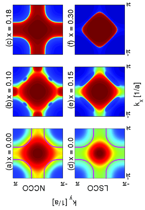
Figure 1: (Color online) Momentum density, $n({\bf k})$ as calculated using Eq. 1 is shown for various dopings for NCCO in (a-c) and for LSCO in (d-f).

Fig. 1 shows maps of $n({\bf k})$ throughout the first Brillouin zone as a function of doping for Nd_2-xCe_xCuO₄ (NCCO) and hole doped La_2-xSr_xCuO₄ (LSCO). In the present NAFL case the combination of self-energy and SDW coherence factors leads to characteristic structures in $n(k)$ at all dopings including half-filling. At half-filling $n({\bf k})$ shows a maximum at the $\Gamma-$point and away from that it decreases gradually and smoothly, from inside to outside the LDA-like FS [magenta solid line in Fig. 1(a) and (d)]. As we dope the system with electrons, the spectral weight increases at the $\Gamma-$point and in addition, $(\pi,0)$ and its equivalent points largely gain spectral weight due to the development of electron pockets in NCCO [Fig. 1(b)]. With further increase of doping, the FS undergoes two topological transitionstanmoyprl ; tanmoysns as also reflected in the momentum density calculations here. The first topological transition in $n({\bf k})$ occurs when the LMB approaches the Fermi level ($E_{F}$) and forms hole-like pockets at $(\pm\pi/2,\pm\pi/2)$. For $x=0.15$, the hole pockets are fully formed and they as well as the electron pockets increase in size with further doping. At $x=0.18$ the electron and hole pockets merge at the hot-spot, the SDW gap collapses, and the full metal-like $n({\bf k})$ appears [second topological transition]. For hole doping, the FS topological transition is complimentary to the electron doped one and here the hole pocket appears first as shown in Fig. 1(e) and above the QCP, the electron-like full FS appears in Fig. 1(f).

A more quantitative account of the effect of self-energy corrections on the residual coherent QP spectral weight is provided in Fig. 2(a), which shows $n({\bf k})$ along high-symmetry lines for NCCO as well as LSCO. Some important effects of correlations on the insulating state should be noted here. At $x=0$, $n[{\bf k}=\Gamma]\approx 0.9$ and $n[{\bf k}=(\pi,\pi)]\approx 0.1$, implying that the self-energy redistributes the spectral weight from the filled states to the unfilled regions even in the insulating phase. PRT [with a different parameter set $t=300$ meV, $t^{\prime}=-t/4$ and $U=12t$] find a similar result $n[{\bf k}=\Gamma]\approx 0.85$paramekanti . At half-filling $n({\bf k})$ is a smoothly varying function throughout the BZ, due to the absence of gapless quasiparticle for both NCCO (green line) and LSCO (not shown). As we increase electron doping, the spectral weight at $\Gamma$ [$(\pi,\pi)$] gradually increases [decreases] whereas the spectral weight increases rapidly at $(\pi,0)$, due to the development of electron pockets, while discontinuities in $n({\bf k})$ arise at the Fermi surface. In the underdoped region, $n({\bf k})$ shows additional singularities along $\Gamma\rightarrow(\pi,0))$ and $(\pi/2,\pi/2)\rightarrow(\pi,\pi)$ due to the presence of shadow bands as marked by gold arrows. Since the shadow bands are usually weak in the cupratesshadow ; chang ; he ; yang1 ; meng , experimental data are available predominantly along the arcs – that is, along the antinodal direction for NCCO and nodal direction for LSCO. These are compared with our theory in Fig. 2(b), effects of the ARPES matrix element notwithstanding.Sahra

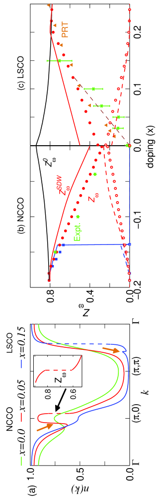
Figure 2: (color online) (a) $n({\bf k})$ for NCCO and LSCO at several representative dopings with dashed lines showing the discontinuous jump at $k_{F}$ (highlighted in inset). Gold arrows mark features from the shadow bands which cross $E_{F}$. (b) $Z_{\omega}$ at $E_{F}$ are shown along the antinodal (red) and nodal (blue) direction for NCCO. Filled (open) symbols give the main (shadow) bands, compared with their corresponding analytical approximation $Z_{\omega}^{SDW}$ plotted by solid (dashed) line of same color. ARPES result (green) is extracted from Ref. nparm, . (c) Same as (b) but for LSCO along the nodal direction. These results are compared with PRT’s calculations for hole dopingparamekanti and ARPES results yoshida for LSCO along the nodal direction. All the experimental data and PRT data in (b) and (c) are normalized to highlight their doping evolution. Brown dashed line shows that if there is nanoscale phase separation in LSCO then $Z_{\omega}$ would scale linearly with doping in the extreme underdoped region.

We define a coherent spectral weight renormalization factor from the discontinuities in $n(k)$:

$$Z_{\omega}=\Delta n(k_{F}),$$ (2)

plotted as a function of doping for NCCO in Fig. 2(b)paramekanti . For the main band in NCCO along the antinodal direction, the UMB crosses the Fermi level at all finite dopings (electron pocket) and $Z_{\omega}$ decreases smoothly with underdoping but vanishes discontinuously at $x=0$. Shown also in Fig. 2(b) is the conventional paramagnetic Green’s function renormalization factor

$$Z_{\omega}^{0}=\left(1-\frac{\partial\Sigma^{\prime}(\omega)}{\partial\omega}\right)_{\omega=0}^{-1}.$$ (3)

It can be seen that the doping dependence in $Z_{\omega}^{0}$ is very weak and strikingly opposite to $Z_{\omega}$. Thus the strong doping dependence of $Z_{\omega}$ is governed by the SDW gap collapse. In Appendix C we derive an approximate analytical form for the SDW corrected renormalization factor $Z_{\omega}^{SDW}$ (at $\omega=0$) in terms of the SDW coherence factors [see Eq. 26]

$$Z_{\omega}^{SDW}=\frac{Z_{\omega}^{0}}{2}\left[1\pm\left(1+\left(\frac{2\Delta}{\xi_{k_{F}}-\xi_{k_{F}+Q}}\right)^{2}\right)^{-1/2}\right].$$ (4)

Note however that $k_{F}$ is the true Fermi momentum in the SDW state, not the LDA one. We see in Fig 2(b) that this simple analytic form captures the essential doping dependence of the full $Z_{\omega}$. As doping increases, the weight of the shadow bands (above the magnetic Brillouin zone) decreases [open symbols in Fig. 2(b)], with the corresponding spectral weight shifting to the main bands. Along the nodal direction, $Z_{\omega}$ remains zero up to optimal doping, and then shows a jump to a slowly increasing value as the LMB crosses the Fermi level. These results are in excellent agreement with experimentnparm .

A similar doping dependence of $Z_{\omega}$ is observed in LSCO along the nodal direction, including the jump at $x=0$ and the spectral weight transfer from the shadow band to the main bandshadow in Fig. 2(b). This is in qualitative agreement with the calculation of PRTparamekanti (triangles in Fig. 2(b)), and with ARPES measurements on LSCOyoshida (open circles) above the optimal doping region. However, in the very underdoped region, the ARPES data seem to extrapolate smoothly to zero at half-filling (dashed line), which may be related to nanoscale phase separations believed to be significant in LSCO.

Note that the analytic renormalization factor $Z_{\omega}^{SDW}$ is defined in the SDW phase, but is treated as a renormalization of the paramagnetic phase dispersion. This subtle point is an attempt to treat the pseudogap physics, and is discussed in more detail in Section IV below.

II.2 FERMI VELOCITY AND DISPERSION RENORMALIZATION

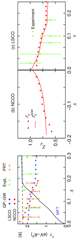
Figure 3: (color online) (a) Fermi velocity $v_{F}$ along the antinodal direction in NCCO and nodal direction in LSCO is compared with ARPES data on LSCOyoshida ; yang and with PRT’s calculationparamekanti . The blue dashed (solid) line gives the corresponding LDA (MFT) results for LSCO. (b) Dispersion renormalization $Z_{d}$ for NCCO along antinodal direction, compared with an approximate analytical formula for the dispersion renormalization $Z_{d}^{SDW}$ (solid line). (c) Same as (b) but for LSCO along the nodal direction. The results are compared with experimental datasahrakorpi .

We turn next to the first order spectral moment $M_{1}({\bf k})$. One can measure the dispersion renormalization from the size of the slope discontinuity, which can be written as (Eq. 27)

$$\Delta\left(dM_{1}({\bf k})/dk\right)_{k_{F}}=Z_{\omega}v_{F},$$ (5)

where $v_{F}$ is the Fermi velocityparamekanti . Knowing $Z_{\omega}$ from Figs. 2(b) and (c), we can extract $v_{F}$ as a function of doping, as seen in Fig. 3(a). The results are obtained for both LSCO and NCCO and compared with ARPES data on LSCOyoshida and with PRT’s variational cluster calculationsparamekanti (hole doping) as well as with LDA and mean-field theory for LSCO. Mean-field results for NCCO have an equivalent doping dependence and thus are not shown here. Notably, in spite of the substantial decrease of $Z_{\omega}$, the QP velocity $v_{F}$ does not diminish on entering into the pseudogap region. Although in the SDW mean field case $v_{F}$ decreases smoothly with underdoping as the gap grows, when a self-energy is introduced, the reduction of the coherent spectral weight ($Z_{\omega}$) with underdoping compensates for this, leading to a net enhancement of $v_{F}$. The results are consistent with PRT and ARPES. Similar results are also obtained in a self-consistent Born approximation with antiferromagnetic pseudogap in the $t-J$ modelPrelovsek .

We define a dispersion renormalization factor in terms of the conventional band velocity with respect to its bare (LDA) counterpart $(v_{F}^{0})$ as

$$Z_{d}=v_{F}/v_{F}^{0},$$ (6)

plotted in Figs. 3(a). In the paramagnetic case, dispersion renormalization is defined as

$$Z_{d}^{0}=Z_{\omega}^{0}Z_{k_{F}}^{0}=Z_{\omega}^{0}\left(1+\partial\Sigma^{\prime}/v_{F}^{0}\partial k\right).$$ (7)

This implies that in a conventional picture the deviation in behavior of $Z_{d}^{0}$ from spectral weight renormalization $Z_{\omega}^{0}$ comes solely from the $k-$dependence of the self-energy. Since this self energy is approximately $k$-independent, one finds $Z_{d}^{0}\approx Z_{\omega}^{0}$. In sharp contrast, the calculated $Z_{d}$ [Fig. 3(b)] shows a strikingly opposite doping dependence to $Z_{\omega}$. This can be understood to be the result of an SDW gap, which introduces a new $k$-dependence in the dispersion renormalization as given by (Eq. 22):

$$Z_{d}^{SDW}=Z_{\omega}^{0}Z_{{\bf k}_{F}}^{SDW}=Z_{\omega}^{0}\left(1+\frac{\Delta^{2}}{\xi_{k_{F}}\xi_{k_{F}+{\bf Q}}}\right).$$ (8)

Figs. 3(b) and (c) compare $Z_{d}$ and $Z_{d}^{SDW}$ for NCCO and LSCO respectively. Thus the doping dependence of $Z_{d}$ implies that as we go towards the Mott insulator, the dispersion tends towards the LDA-bands, consistent with LSCO results (blue open circles)sahrakorpi . The opposite doping dependences of $Z_{d}$ and $Z_{\omega}$ can be readily understood by comparing the corresponding analytical formulas $Z_{d}^{SDW}$ (Eq. 8) and $Z_{\omega}^{SDW}$ (Eq. 4). $Z_{d}^{SDW}~{}(Z_{\omega}^{SDW})$ varies with SDW gap as $\Delta~{}(1/\Delta)$, increasing (decreasing) with underdoping. This in turn moves the in-gap states further away from the Fermi level (hence decreasing $Z_{\omega}$), and thus shifting the band towards the LDA values (increasing $Z_{d}$)tanmoysw .

III Specific heat

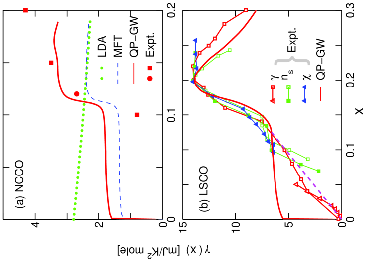
Figure 4: (color online) (a) Specific heat coefficient $\gamma(x)$ for different theoretical calculations (various lines), and the experimental results on NCCO (red squares)brugger and PLCCO (red circles)li . (b) Same as (a) but for LSCO (red squaresyoshida and triangleskomiya ). Results are compared with $n_{s}$ [filled green squaresyoshida and open green squaresyang ] and $\chi$ (blue)ino ), all normalized at the VHS. The red dashed line shows that in underdoped LSCO $\gamma$ scales linearly with doping. Theoretical $\gamma$ has been scaled by a factor of 1.1, consistent with a weak electron-phonon renormalization.

A striking application of the renormalization effects can be seen in the doping evolution of the specific heat. A general expression for the specific heat $c_{V}$ in the SDW state including the self-energy correction is given in Appendix D. We find that the Sommerfeld coefficient $\gamma$ can be well described in terms of the density of state (DOS) ($N(0)$) in the SDW state asabrikosov ,

$$\gamma=c_{V}(T)/T\approx\frac{2\pi^{2}k_{B}^{2}}{3}N(0)/Z_{\omega}^{0},$$ (9)

where $N_{0}(0)$ is the mean-field DOS with SDW gap but without self energy corrections.

Fig. 4 compares experimental values of $\gamma$ as a function of doping in LSCOyoshida ; komiya and electron doped NCCObrugger and Pr_1-xLaCe_xCuO₄ (PLCCO)li with several calculations including bare LDA, MFT results with SDW gap, and with self-energy correction for both NCCO and LSCO. The striking differences between NCCO and LSCO away from half-filling are due to the presence of the van-Hove singularity (VHS) near $E_{F}$ in the latter case. $N(0)$ in LDA thus decreases (from a finite value at $x=0$) with increasing electron doping, whereas for LSCO $N(0)$ has a peak at the doping corresponding to the VHS $x_{VHS}\sim 0.20$sahrakorpi . SDW order opens a gap, reducing $N(0)$, and introduces steps associated with the collapse of the SDW gap. Thus, for electron doping $N(0)$ is nearly flat for $x<0.11$, reflecting the quasi-two dimensionality of the electron pocket (constant DOS) in cuprates. The step at $x\sim 0.11$ signals the appearance of the hole pocket. Similarly in LSCO the appearance of the electron pocket near $(\pi,0)$ at $x\approx 0.17$ within our model greatly enhances the VHS features. Finally, adding self-energy corrections (in the form of $1/Z_{\omega}^{0}$) preserves the general shape of the SDW $\gamma$, while shifting its magnitude back towards the LDA values. It is interesting to relate the doping dependence of $\gamma(0)$ and $Z_{\omega}$ in Fig. 2(b). Note that $Z_{\omega}$ is evaluated at a particular Fermi momentum whereas $\gamma(0)$ is computed after summing over $Z_{\omega}$ at all $k_{F}$. As $Z_{\omega}$ exhibits complimentary doping dependencies for main and shadow bands, so the total remains fairly constant. These results are in striking contrast to the strong coupling limit where $\gamma$ should diverge with the effective mass as $x\rightarrow 0$.KOg

The agreement with experiment is quite good in LSCO for $x\geq 0.10$, including the strong VHS feature. Interestingly, the superfluid density $n_{s}$ and the paramagnetic susceptibility data, which are proportional to the total FS areas, show a similar doping dependence to $\gamma$. However, below $x=0.10$ $\gamma\rightarrow 0$ as $x\rightarrow 0$, an effect not captured by our calculations. Such an effect could be due to a Coulomb gapkomiya and/or nanoscale phase separation. The linear dashed line in Fig. 3(b) illustrates the corrected form expected in the latter case. Note that nanoscale phase separation would produce the dashed line seen in Fig. 2(c) as well as explain the anomalous doping dependence of the chemical potential.FIMT Hence the enhanced gossamer features seen in LSCO may be related to nanoscale phase separation.

IV discussion

The present calculations are most appropriate for electron doping, where only the $(\pi,\pi)$ commensurate SDW order is observed, and the model is in very good agreement with experiment. Remarkably, the same model when applied to hole-doped cuprates describes many aspects of the two-gap scenariotanmoytwogap ; AndHir , despite the fact that it does not capture the incommensurate magnetization. The non-Fermi-liquid behavior presented here is not sensitive to the specifics of the competing order, but only to the resulting superlattice $q$-vector. We have analyzed other candidates for the competing order including charge, flux, or $d-$density wavestanmoytwogap , and find that the results are insensitive to the nature of the competing order state. Thus, Eqs. 4 and 8 continue to hold for any $Q=(\pi,\pi)$ order, as long as the appropriate gap $\Delta$ is used.

In the presence of long-range magnetic order, the Green’s function develops a second pole, and should properly be treated as a tensor. However, the pseudogap phase is more likely to be associated with only short range order, in which case the second pole does not cross the real axis, the Green’s function can be treated as a scalar, and the information about incipient gap formation is encoded in the self-energy.MKII The analytic approximations of Eqs. 4 and 8 mimic this effect by treating the renormalization factors as acting on the paramagnetic dispersion $\xi_{{\bf k}}$, with information on proximity to long-range magnetic order encoded into $Z_{\omega}^{SDW}$ and $Z_{d}^{SDW}$.

This approach is similar to the phenomenological model introduced by Yang et al.YRZ to describe RVB physics. Indeed, their phenomenological self energy is quite similar to the form expected for a NAFL, except for the treatment of scattering at the magnetic zone boundary, which splits the pockets expected for AF order into two half-pockets. One puzzle is that the effect of strong scattering at a superlattice zone boundary is already well understood in standard Lifshitz-Kosevich theorymagb , where it leads to a quantum switching between arcs of Fermi surface. This produces harmonic mixing frequencies in a quantum oscillation (QO) spectrum, and it is hard to see how it could evolve into the short-circuiting effect of Yang, et al. At any rate, the QOs observed in NCCO are more consistent with the present model.qohelm

V conclusion

In conclusion, we have shown that a number of salient features of the non-Fermi-liquid state of the underdoped cuprates can be understood within the framework of a competing density wave order, which breaks the particle-hole symmetry, and drives reconstruction of the FS. We provide a transparent and analytic basis for describing how the non-Fermi-liquid effects play out in renormalizing spectral weight via $Z_{\omega}$ and electronic dispersion via $Z_{d}$, and how they conspire to yield a specific heat in the cuprates which is essentially conventional in nature at all dopings. Our framework would provide a straightforward basis for understanding how the broken-symmetry order leads to ‘non-Fermi-liquid’ effects, not only in the cuprates, but also in heavy-fermionsaronson , Fe-based superconductorsxu and other strongly correlated materials.

Appendix A Details of quasiparticle-GW (QP-GW) Model

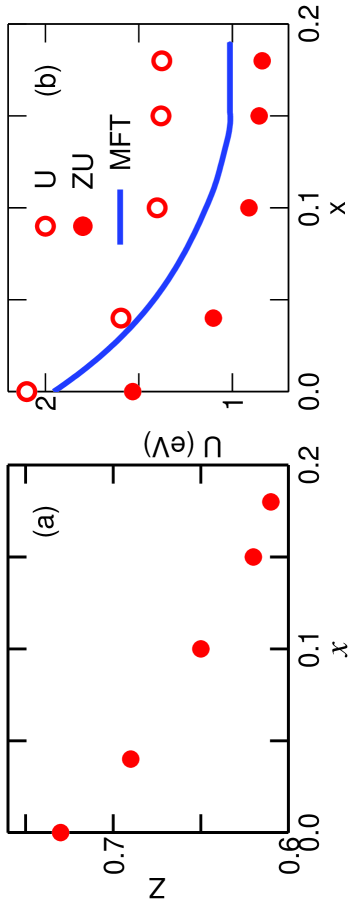
Figure 5: (color online) (a) Average renormalization factor $Z$ decreases linearly with doping, very much like $Z_{\omega}^{0}$ in Figs. 2(b) and (c). (b) Our computed doping dependence of selfconsistent values of $U$ and $ZU$ is compared with earlier mean field resultskusko ; tanmoyprl .

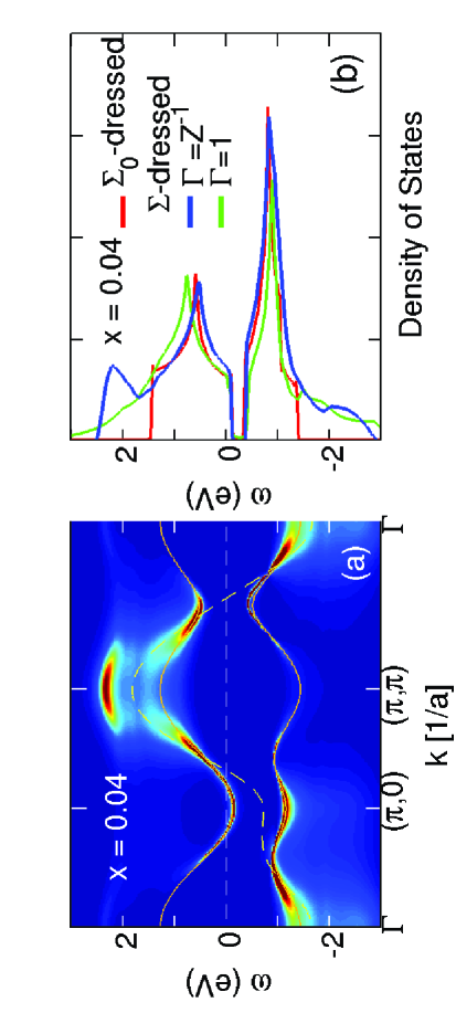
Figure 6: (color online) (a) Spectral intensity as a function of $\omega$ along the high-symmetry lines for several dopings (at temperature $T=0$). Blue to red color map gives the minimum to maximum intensity. The yellow dashed line gives the underlying LDA dispersion where the gold lines represent the renormalized magnetic bands ($\Sigma_{0}$-dressed). (b) The QP-GW DOS (blue lines) is compared with $\Sigma_{0}$-dressed DOS (red line) calculated at $T=0$. The green lines show the DOS without the vertex correction.

In the QP-GW formalism the bare dispersion is taken as the LDA dispersion ($\xi_{{\bf k}}=\epsilon_{{\bf k}}-E_{F}$), modeled via a tight-binding (TB) fitmarkietb ; foot2 ; ft_sophi1 ; ft_sophi3 ; ft_sophi4 . We calculate the self-energy in a GW-like formalism using a simplified (one parameter) scheme where the input and final self-energies are self-consistent in the coherent part only (QP-GW model).

In the following, we use a ‘tilde’ over a quantity to symbolize that it is a $2\times 2$ matrix. The self-energy in the underdoped region is written in canonical form using the Nambu formalism as

$$\tilde{\Sigma}^{t}({\bf k},\sigma,i\omega_{n})=\tilde{\Sigma}({\bf k},\sigma,i\omega_{n})+\phi({\bf k},\sigma,i\omega_{n})\tilde{\tau_{1}}.$$ (10)

The dressed Green’s function is then

$$\tilde{G}^{-1}({\bf k},\sigma,i\omega_{n})=i\omega_{n}\tilde{1}-\tilde{H}_{LDA}-\tilde{\Sigma}^{t}({\bf k},\sigma,i\omega_{n})$$ (11)

where $\tilde{H}_{LDA}$ is the bare Hamiltonian defined in the magnetic zone as $diag[\xi_{{\bf k}},~{}\xi_{{\bf k}+{\bf Q}}]$, and the $\tilde{\tau}_{i}$ are Pauli matrices. At each step, we adjust the chemical potential $E_{F}$ to fix the doping. Real frequency Green’s functions are extracted from the Matsubara results by analytic continuation $i\omega_{n}\rightarrow\omega+i\delta$. Here, $\tilde{\Sigma}({\bf k},\sigma,i\omega_{n})$ is a $2\times 2$ matrix in the SDW stateSWZ , whose diagonal part renormalizes $\tilde{H}_{LDA}$, while the off-diagonal term gives a (small) anomalous frequency dependence to the gap function $\phi({\bf k},\sigma,i\omega_{n})=\sigma\Delta$. $\Delta=US$ is the magnetic gap parameter and $S$ is the magnetization at the commensurate vector ${\bf Q}=(\pi,\pi)$ for Hubbard $U$, which is calculated using a mean-field approximationtanmoytwogap . The doping dependence of the on-site Hubbard $U$ is obtained due to charge screening from $U=\left<V(q)/(1+V(q)\chi(q)\right>$, where $V(q)$ is the long-range Coulomb interactionmarkiecharge , and $\chi(q)$ is the charge susceptibility in the $\phi-$gapped state defined below. The obtained values of screened $U$ are given in Ref. tanmoyop, and plotted in Fig. 5(b).

We calculate the self energy due to the spin as well as the charge response within a GW framework as

$$\tilde{\Sigma}({\bf k},\sigma,i\omega_{n})=\frac{3}{2}U^{2}Z\sum_{{\bf q},\sigma^{\prime}}^{\prime}\int_{-\infty}^{\infty}\frac{d\omega_{p}}{2\pi}$$

$$\tilde{G}({\bf k}+{\bf q},\sigma^{\prime},i\omega_{n}+\omega_{p})\Gamma({\bf k},{\bf q},i\omega_{n},\omega_{p}){\rm Im}[\tilde{\chi}_{\rm RPA}^{\sigma\sigma^{\prime}}({\bf q},\omega_{p})],$$

where the prime over the momentum summation indicates that the summation is restricted within the magnetic Brillouin zone. The dressed susceptibility in the above equation is given in terms of the $2\times 2$ RPA susceptibility as,SWZ

$$\tilde{\chi}_{\rm{RPA}}^{\sigma\sigma/\sigma\bar{\sigma}}({\bf q},i\omega_{n})=\frac{\tilde{\chi}_{0}^{\sigma\sigma/\sigma\bar{\sigma}}({\bf q},i\omega_{n})}{\tilde{{\bf 1}}\pm U\tilde{\chi}_{0}^{\sigma\sigma/\sigma\bar{\sigma}}({\bf q},i\omega_{n})}.$$ (13)

Here the superscript $(\sigma\sigma)$ refers to the combined charge plus longitudinal spin susceptibility tensor, whereas $(\sigma\bar{\sigma})$ (with $\bar{\sigma}=-\sigma$) gives the transverse susceptibility tensor, and the $\tilde{\chi}_{0}^{\sigma\sigma/\sigma\bar{\sigma}}({\bf q},i\omega_{n})$ are bare susceptibilities.


A self-consistent ‘dressed’ GW calculation would include $\Sigma$ on the right-hand side of Eq. A in both $G$ and $\chi_{0}$. This generally leads to problems unless a vertex correction $\Gamma$ is included. Improved results are often found by using a ‘bare’ $G_{0}$ and $\chi_{0}$ – bare in the sense of not including $\Sigma$. This latter $G_{0}W_{0}-$scheme also fails in the present calculation by producing too large a renormalization of the band dispersion. This is because the imaginary part of the bare susceptibility has the form $\chi_{0}^{\prime\prime}\sim\delta(\omega-[\xi_{k+q}-\xi_{k}])$, so that near the Fermi surface, $\chi_{0}^{\prime\prime}$ should scale in frequency with the dressed quasiparticle dispersion. Since $G_{0}W_{0}$ uses the bare dispersions, peaks in $\chi_{0}^{\prime\prime}$, which control the renormalization, lie at too high an energy.

We therefore introduce a modified, or ‘quasiparticle’ (QP) GW approximationwater3 for the right-hand side (RHS) of Eq. A, as follows. In Eq. A, we dress both $G_{0}$ and $\chi_{0}$ with an ‘input’ self-energy chosen as

$$\tilde{\Sigma}(i\omega_{n})=(1-1/Z)i\omega_{n}\tilde{1}.$$ (14)

Thus, the input $\Sigma$ contains a single parameter $Z$, which gives an overall renormalization of the ‘input’ dispersions (RHS of Eq. A). With this approximation, the bare susceptibilities become

$$\tilde{\chi}_{0}^{{\sigma\sigma}/{\sigma\bar{\sigma}}}({\bf q},i\omega_{n})=-Z^{2}\sum_{{\bf k}}^{\prime}\sum_{\nu,\nu^{\prime}}\tilde{S}_{\nu,\nu^{\prime}}^{\sigma\sigma/\sigma\bar{\sigma}}\frac{f(Z{E}^{\nu}_{{\bf k}})-f(Z{E}^{\nu^{\prime}}_{{\bf k}+{\bf q}})}{i\omega_{n}+Z{E}^{\nu}_{{\bf k}}-Z{E}^{\nu^{\prime}}_{{\bf k}+{\bf q}}}.$$

The prime over the summation has the same meaning as in Eq. A. In Eq. A, the $\nu$ summation is over the two magnetic bands UMB ($\nu=+$) and LMB ($\nu=-$):

$$E_{{\bf k}}^{\pm}=(\xi_{{\bf k}}^{+}\pm E_{0{\bf k}})$$ (16)

with $\xi_{{\bf k}}^{\pm}=(\xi_{{\bf k}}\pm\xi_{{\bf k}+{\bf Q}})/2$ and $E_{0{\bf k}}=\sqrt{(\xi_{{\bf k}}^{-})^{2}+\Delta^{2}}$ (Ref. tanmoysw, ), $f(E)=1/(1+\exp{(E/k_{B}T)})$ is the Fermi function at temperature $T$, and $k_{B}$ is the Boltzmann constant. The coherence factors $\tilde{S}_{\nu,\nu^{\prime}}^{\sigma\sigma/\sigma\bar{\sigma}}$ give the amplitude of the scattering of the quasiparticles with the charge and magnon modes of the system respectively with components

$$\tilde{S}_{\nu,\nu^{\prime}}^{\sigma\sigma/\sigma\bar{\sigma}}(11) = (\alpha_{{\bf k}}\alpha_{{\bf k}+{\bf q}}\pm\nu\nu^{\prime}\beta_{{\bf k}}\beta_{{\bf k}+{\bf q}})^{2},$$

$$\tilde{S}_{\nu,\nu^{\prime}}^{\sigma\sigma/\sigma\bar{\sigma}}(12) = -\nu(\alpha_{{\bf k}}\beta_{{\bf k}}\pm\nu\nu^{\prime}\alpha_{{\bf k}+{\bf q}}\beta_{{\bf k}+{\bf q}}).$$ (17)

Here

$$\alpha_{{\bf k}}(\beta_{{\bf k}})=\sqrt{\frac{1}{2}\left(1\pm\frac{\xi_{{\bf k}}^{-}}{E_{0{\bf k}}}\right)}$$ (18)

respectively are the weights associated with the U/LMBs. The other coherence factors in Eq. A can be derived using the translational symmetry with respect to ${\bf q}$.

A limitation of the present scheme is also apparent from Eq. A. This self-energy is a good approximation for the coherent, dressed bands, but does not extend to the incoherent part of the spectrum, thereby underestimating the incoherent spectral weight. We have empirically found that this can be partly remedied by incorporating a vertex function $\Gamma$. Consistent with the QP approximation, the vertex correction to the self-energy is obtained through Ward’s identity as

$$\Gamma({\bf k},{\bf q},i\omega_{n},\omega_{p}) = 1-(\partial\Sigma^{\prime}/\partial\omega)_{\omega=\omega_{0}}=1/Z.$$ (19)

Even though we have chosen perhaps the simplest form of the vertex correction, it has a large impact on the spectral weight transfer. $\Gamma=1/Z$ eventually reduces the renormalization of the bare susceptibility in Eq. A and hence the spectral weight is spread out more towards higher energies, enhancing the incoherent spectral weight. An illustration of the importance of this vertex correction is given in Fig. 6(b).

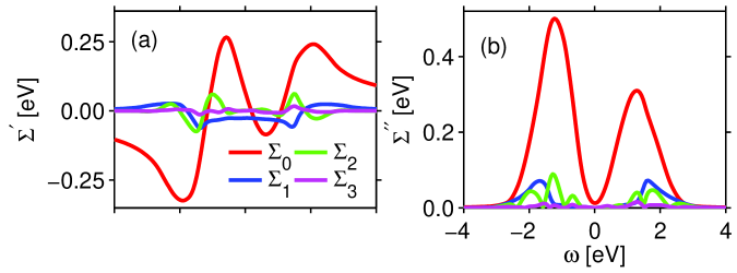
Figure 7: (color online) Real and imaginary part of the self-energy as expanded in the tight-binding form of Eq. A11.

Next we discuss our self-consistent scheme, and explain how the parameter $Z$ is chosen. We choose $Z$ to match the average renormalization in the low-energy (coherent) part of the spectrum. Specifically, if $\Sigma^{\prime}$ is the real part of the diagonal self energy, then we adjust $Z$ self-consistently until it satisfies $Z=(1-\partial\Sigma^{\prime}/\partial\omega)^{-1}_{\omega=\omega_{o}}$, where $\omega_{o}$ is an average quasiparticle excitation energy, which is related to the poles in $G$. This gives a good self-consistent result for the coherent spectral weight in the low-energy region (see Fig. 6(a)), whereas the incoherent parts in the higher energy regions are not self-consistent. Thus our scheme is in the spirit of Landau’s quasiparticles, except that Landau assumed that all of the spectral weight goes into the QP band, while we have only a fraction $Z$.

When this is done, we find that $U$ is effectively further renormalized by the doping dependent $Z$ [Fig. 5(a)], so that the product $U\chi_{0}$ is approximately independent of $Z$. The resulting $ZU$ closely resembles our earlier mean-field calculations as shown in Fig. 5(b).

Lastly, we find that the momentum dependence of the fluctuation self-energy $\Sigma$ is relatively weakwater3 ; jarrell . To emphasize this point, we expanded the momentum dependence of the self energy in a form similar to the tight-binding model:

$$\Sigma(\omega,{\bf k}) = \Sigma_{0}(\omega)+\Sigma_{1}(\omega)\left(c_{x}+c_{y}\right)$$ (20)

$$+\Sigma_{2}(\omega)c_{x}c_{y}+\Sigma_{3}(\omega)\left(c_{2x}+c_{2y}\right),$$

where $c_{\alpha(x/y)}=\cos{(\alpha k_{(x/y)}a)}$. We calculate the self-energy at four high symmetry points ${\bf k}=(0,0),~{}(\pi,0),~{}(\pi,\pi)~{}{\rm and}~{}(\pi/2,\pi/2)$ to obtain the above coefficients as shown in Fig. 7. Clearly, only the $k-$independent part (red line) has a strong contribution. Therefore, we have simplified the self-energy calculation by approximating it with a $k$-independent average value taken as the value at $k=(\pi/2,\pi/2)$. Since we are neglecting the $k-$dependence of the self energy, $\Sigma_{11}=\Sigma_{22}$ and $\Sigma_{12}=\Sigma_{21}$.

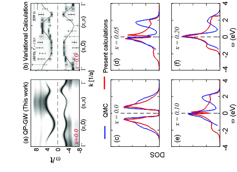
Figure 8: (color online) (a) The spectral intensity of NCCO at $x=0$, plotted (in logarithmic scale) along the high-symmetry lines, is compared with variational calculationsgrober in (b). (c)-(f) The computed DOS at various dopings are compared with the corresponding QMC results (blue lines) for x = 0.0 [Ref. maier, ] and for x = 0.05 to x = 0.20 [Ref. jarrell, ].

Figure 8(a) shows that in the QP-GW scheme the spectral weight splits up into four band-like features. The two bands closer to the Fermi level are the UMB and LMB, associated with the development of the spin-density wave (SDW). The residual incoherent spectral dispersions at higher energies are the UHB and LHB. Similar four band features are found in the variational cluster calculations shown in Fig. 8(b)grober . The corresponding density of states (DOS) shows four peaks associated with these four bands, Figs. 8(c)-(f). These four band features separated by SDW gap or ‘waterfall’ effects show semi-quantitative agreement with QMC resultsmaier ; jarrell . With doping, the two magnetic bands merge in a QCP near optimal doping, while the two Hubbard bands occur at the top and bottom of the LDA bands, and hence the associated Hubbard band splitting is comparable to the LDA bandwidth at all dopings.

Appendix B Summary of renormalization factors

We summarize the various renormalization factors that arise in this study for convenience reference. Equation numbers in square brackets indicate where a specific factor is discussed in the text.

$$Z_{\omega} = \Delta n(k_{F})\qquad\qquad\qquad\qquad\qquad\qquad[\text{Eq.~{}\ref{Zw}}]$$

$$= {\rm Total~{}spectral~{}weight~{}renormalization}.$$

$$Z_{\omega}^{0} = \left(1-\partial\Sigma^{\prime}/\partial\omega\right)_{\omega=0}^{-1}\qquad\qquad\qquad\quad[\text{Eq.~{}\ref{Zw0}}]$$

$$= {\rm Self~{}energy~{}contribution~{}to~{}spectral~{}weight}$$

$${\rm renormalization}.$$

$$Z_{\omega}^{SDW} = \frac{Z_{\omega}^{0}}{2}\left[1\pm\left(1+\left(\frac{2\Delta}{\xi_{k_{F}}-\xi_{k_{F}+Q}}\right)^{2}\right)^{-1/2}\right]$$

$$\qquad\qquad\qquad\qquad\qquad\qquad\qquad[\text{Eq.~{}\ref{ZwAF}}]$$

$$=$$ Analytical formula for SDW spectral weight

$${\rm renormalization}.$$

$$Z_{d} = v_{F}/v_{F}^{0}\qquad\qquad\qquad\qquad\qquad\qquad[\text{Eq.~{}\ref{Zd}}]$$

$$= {\rm Velocity~{}renormalization.}$$

$$Z_{d}^{0} = Z_{\omega}^{0}Z_{\bf k}^{0}=Z_{\omega}^{0}\left(1+{\partial\Sigma^{\prime}}/{v_{F}^{0}\partial k}\right)\qquad\quad[\text{Eq.~{}\ref{Zd0}}]$$

$$= {\rm Conventional~{}dispersion~{}renormalization.}$$

$$Z_{d}^{SDW} = Z_{\omega}^{0}\left(1+{\Delta^{2}}/{\xi_{k_{F}}\xi_{k_{F}+Q}}\right)\qquad\qquad\qquad[\text{Eq.~{}\ref{ZdAF}}]$$

$$= {\rm Analytical~{}formula~{}for~{}SDW~{}dispersion}$$

$${\rm renormalization.}$$

$$\gamma = c_{V}/T\qquad\qquad\qquad\qquad\qquad\qquad\qquad[\text{Eq.~{}\ref{gamma}}]$$

$$= {\rm Specific~{}heat~{}coefficient.}$$

Appendix C Analytical form of various renormalization factors

Near the Fermi level, the dressed Green’s functions from Eq. 11 can be approximated as,

$$G_{11}({\bf k},\omega) = Z^{0}_{\omega}\frac{\omega-\bar{\xi}_{{\bf k}+{\bf Q}}}{(\omega-\bar{\xi}_{{\bf k}})(\omega-\bar{\xi}_{{\bf k}+{\bf Q}})+(\overline{\Delta})^{2}}$$ (21)

$$= \frac{Z^{0}_{\omega}}{\omega-Z_{d}^{SDW}({\bf k})\xi_{{\bf k}}}$$

where $\bar{\xi}_{{\bf k}}=Z^{0}_{\omega}\xi_{{\bf k}}$, $\overline{\Delta}=Z_{\omega}^{0}\Delta$, and $\xi_{{\bf k}}$ is the bare (LDA) dispersion calculated at the same doping. In Eq. 21, $Z^{0}_{\omega}=(1-\partial\Sigma_{11}^{\prime}(\omega)/\partial\omega)^{-1}$ (Eq. 3) is the part of the spectral weight renormalization due to the self-energy, where we have neglected the contribution of $\Sigma_{12}$. Even though we assume a $k-$independent self-energy and thus $Z_{{\bf k}}^{0}=1$ from Eq. 21, the SDW gap introduces a $k-$dependent dispersion renormalization (defined here at $\omega=0$) given by

$$Z_{d}^{SDW}({\bf k})=Z_{\omega}^{0}\left(1+\frac{\Delta^{2}}{\xi_{{\bf k}}\xi_{{\bf k}+{\bf Q}}}\right).$$ (22)

Note that $\xi_{{\bf k}}$, $~{}\xi_{{\bf k}+{\bf Q}}$, and $\Delta$ are all bare values in Eq. 22 as the same renormalization factor $Z_{\omega}^{0}$ gets cancelled out in the last term. Furthermore, we can split the spectral function $A({\bf k},\omega)={\rm Im}G({\bf k},\omega)/\pi$ into a coherent part (at Fermi level) and an incoherent part where the former can be represented by a delta function as

$$A_{11}({\bf k},\omega) = Z_{\omega}^{0}\left(\alpha_{{\bf k}}^{2}\delta(\omega-\bar{E}^{+}_{{\bf k}})+\beta_{{\bf k}}^{2}\delta(\omega-\bar{E}^{-}_{{\bf k}})\right)_{\omega=0}$$ (23)

$$+ A_{incoh}({\bf k},\omega>0)$$

where $\bar{E}_{{\bf k}}^{\pm}=Z_{\omega}^{0}E_{{\bf k}}^{\pm})$. Therefore, the coherent part is governed by the SDW coherence factors $\alpha_{{\bf k}}$ and $\beta_{{\bf k}}$ for the filled state with a renormalization by $Z_{\omega}^{0}$. The zeroth and first order moment of the spectral weight (Eq. 1) then can be approximated respectively asparamekanti ,

$$n({\bf k}) = \int_{-\infty}^{0}A_{11}({\bf k},\omega)d\omega$$ (24)

$$\approx Z_{\omega}^{0}\left[\alpha_{{\bf k}}^{2}\theta(-\bar{E}_{{\bf k}}^{+})+\beta_{{\bf k}}^{2}\theta(-\bar{E}_{{\bf k}}^{-})\right]$$

$$M_{1}({\bf k}) = \int_{-\infty}^{0}A_{11}({\bf k},\omega)\omega d\omega$$

$$\approx Z_{\omega}^{0}({\bf k}-{\bf k}_{F})\left[\alpha_{{\bf k}}^{2}v_{F}^{+}\theta(-\bar{E}_{{\bf k}}^{+})+\beta_{{\bf k}}^{2}v_{F}^{-}\theta(-\bar{E}_{{\bf k}}^{-})\right].$$

In the second equation above, we have expanded the renormalized band near the Fermi level as $\bar{E}_{{\bf k}}^{\pm}\approx v_{F}^{\pm}({\bf k}-{\bf k}_{F})$, where $v_{F}$ is the corresponding Fermi velocity. The singularity in $n({\bf k})$ becomes

$$Z_{\omega}=\Delta n({\bf k}_{F}) = Z_{\omega}^{0}\alpha_{{\bf k}_{F}}^{2}\equiv Z_{\omega}^{+}\qquad\text{for UMB}$$

$$= Z_{\omega}^{0}\beta_{{\bf k}_{F}}^{2}\equiv Z_{\omega}^{-}\qquad\text{for LMB}.$$ (26)

Note that in the present case, the weight for UMB (LMB) appears along the antinodal (nodal) direction when the band crosses the Fermi level. Inserting the form of $\alpha,~{}\beta$ from Eq. 18, we get Eq. 4. Similarly, inserting this $Z_{\omega}$ in Eq. LABEL:A2M1, we can measure the singular jump in $M_{1}({\bf k})$ as

$$\Delta\left(dM_{1}({\bf k})/d{\bf k}\right) = Z_{\omega}^{\pm}v_{F}^{\pm}.$$ (27)

Thus $Z_{\omega}$ and $v_{F}$ acquire a $k$-dependence through the SDW coherence factor.

Appendix D Specific Heat Calculation

Following the derivation by Abrikosov et. al. abrikosov , we calculate the entropy in the SDW state for a strongly correlated system at finite temperature (in the low temperature limit) as

$$S(T) = -\frac{2\beta k_{B}^{2}}{2\pi i}\int_{-\infty}^{\infty}d\omega\omega\left(-\frac{\partial f(\omega)}{\partial\omega}\right)$$

$$~{}\times\sum_{{\bf k},\sigma}{\rm Tr}\left[\ln{\tilde{G}_{R}^{-1}({\bf k},\sigma,\omega)}-\ln{\tilde{G}_{A}^{-1}({\bf k},\sigma,\omega)}\right].$$

Here the $2\times 2$ retarded and advanced (dressed) Green’s functions $G_{R}/G_{A}$ depend on the temperature through the SDW order parameter only, which has a very weak dependence in the low temperature region. We can rewrite Eq. D in terms of a dimensionless parameter $y=\beta\omega$ following Ref. toschi, , and then taking the temperature derivative we get the expression for the specific heat as

$$c_{V}(T)=-\frac{k_{B}\beta^{2}}{4\pi}\int_{-\infty}^{\infty}dyy^{2}~{}{\rm{sech}}^{2}(y/2)~{}~{}~{}~{}~{}~{}~{}~{}~{}~{}~{}~{}~{}~{}~{}~{}~{}~{}~{}~{}~{}~{}$$

$$~{}\times\sum_{{\bf k},\sigma}{\rm Tr}\left[{\rm Im}\left(\tilde{G}_{R}({\bf k},\sigma,\omega)\frac{\partial}{\partial\omega}\tilde{G}_{R}^{-1}({\bf k},\sigma,\omega)\right)\right]_{\omega=y/\beta}.$$

$c_{V}(T)$ behaves linearly with $T$ in the low temperature region, while the slope ($\gamma$) undergoes an abrupt change with a kink in the waterfall region. Since the high energy kink energies for cuprates are around 0.3 to 0.6 eV, the kink should appear in $c_{V}$ only at a very high temperature, $T_{k}\sim 10^{3}K$. Thus, in our calculation of $\gamma$ (Fig. 5), we have used the full expression for $c_{V}$ above but evaluated it in the $\omega=0$ limit.

In the $T=0$ ($\omega\rightarrow 0$) limit, Eq. D can be simplified as $\rm{sech}(y)=\delta(y-\beta\omega)$. In this limit, the imaginary part of the self-energy is zero and thus the last quantity in Eq. D is calculated by noting that the $\omega-$derivative of the real part of the self-energy is: diagonal term = $1-1/Z_{\omega}^{0}$, and off-diagonal term =$(\partial\Sigma^{\prime}_{12}/\partial\omega)_{\omega=0}$. This simplifies Eq. D as

$$c_{V} \approx \frac{2}{3}\pi^{2}k_{B}^{2}T\sum_{{\bf k}}\left[\frac{1}{Z_{\omega}^{0}}\left(A_{11}({\bf k},0)+A_{22}({\bf k},0)\right)\right.$$ (30)

$$\left.+\frac{\partial\Sigma_{12}}{\partial\omega}\left(A_{12}({\bf k},0)+A_{21}({\bf k},0)\right)\right],$$

where $A_{11}$ is given in Eq. 23 and $A_{22}=A_{11}({\bf k}\rightarrow{\bf k}+{\bf Q})$, i.e., $A_{22}$ is similar to $A_{11}$, only the weights ($\alpha_{{\bf k}}^{2}$, $\beta_{{\bf k}}^{2}$) are interchanged. We have used Eq. 30 in the calculation of Fig. 5. The constraint $\alpha_{{\bf k}}^{2}+\beta_{{\bf k}}^{2}=1$ removes these SDW coherence factors from the equation. Neglecting the off-diagonal term proportional to the small quantity $\partial\Sigma_{12}/\partial\omega$, the specific heat expression becomes

$$c_{V} \approx \frac{2}{3}\pi^{2}k_{B}^{2}T\sum_{{\bf k}}\left[\delta(-Z_{\omega}^{0}E_{{\bf k}}^{+})+\delta(-Z_{\omega}^{0}E_{{\bf k}}^{-})\right]+...$$ (31)

$$\approx \frac{2}{3}\pi^{2}k_{B}^{2}T\left[N^{+}(0)+N^{-}(0)\right]/Z_{\omega}^{0}.$$

Here, $N^{\pm}(0)=\sum_{{\bf k}}\delta(-E_{{\bf k}}^{\pm})$ is the total density of states for the (U/L)MBs at the Fermi level in the SDW state, but without renormalization (mean-field theory). For both NCCO and LSCO, Eq. 31 is an excellent approximation to the exact expression of Eq. 30. It is interesting to observe that in the final expression for $c_{V}$ (Eq. 31), the self energy correction enters only through the renormalized DOS. Thus, in the QP-GW model, $c_{V}$ has the same form as in conventional Fermi-liquid theory.

References

- (1) S. Sahrakorpi, R. S. Markiewicz, Hsin Lin, M. Lindroos, X. J. Zhou, T. Yoshida, W. L. Yang, T. Kakeshita, H. Eisaki, S. Uchida, Seiki Komiya, Yoichi Ando, F. Zhou, Z. X. Zhao, T. Sasagawa, A. Fujimori, Z. Hussain, Z.-X. Shen, and A. Bansil, Phys. Rev. B 78, 104513 (2008).
- (2) T. Yoshida, X. J. Zhou, K. Tanaka, W. L. Yang, Z. Hussain, Z.-X. Shen, A. Fujimori, S. Sahrakorpi, M. Lindroos, R. S. Markiewicz, A. Bansil, Seiki Komiya, Yoichi Ando, H. Eisaki, T. Kakeshita, and S. Uchida, Phys. Rev. B 74, 224510 (2006).
- (3) T Yoshida, X J Zhou, D H Lu, Seiki Komiya, Yoichi Ando, H Eisak4, T Kakeshita, S Uchida, Z Hussain, Z-X Shen and A Fujimori J. Phys.: Cond. Mat. 19, 125209 (2007).
- (4) R.B. Laughlin, cond-mat:0209269 (unpublished); F.C. Zhang, Phys. Rev. Lett. 90, 207002 (2003).
- (5) R.S. Markiewicz, S. Sahrakorpi, and A. Bansil, Phys. Rev. B 76, 174514 (2007).
- (6) A. Macridin, M. Jarrell, Thomas Maier, and D. J. Scalapino, Phys. Rev. Lett 99, 237001 (2007).
- (7) S. Komiya and I. Tsukada, arXiv:0808.3671.
- (8) T. Brugger, T. Schreiner, G. Roth, P. Adelmann, and G. Czjzek, Phys. Rev. Lett. 71 2481 (1993).
- (9) Shiliang Li, Songxue Chi, Jun Zhao, H.-H. Wen, M. B. Stone, J. W. Lynn, and Pengcheng Dai, Phys. Rev. B 78, 014520 (2008).
- (10) T. Senthil and P.A. Lee, Phys. Rev. Lett. 103, 076402 (2009).
- (11) S. Sachdev, Max A. Metlitski, Yang Qi, and Cenke Xu Phys. Rev. B 80, 155129 (2009).
- (12) N. S. Vidhyadhiraja, A. Macridin, C. Aźen, M. Jarrellaz, and Michael Ma, Phys. Rev. Lett. 102, 206407 (2009) .
- (13) S. Sakai, Yukitoshi Motome, and Masatoshi Imada, Phys. Rev. Lett. 102 056404 (2009).
- (14) P. Wröbel, A. Maciag, and R. Eder et. al. J. Phys.: Cond. Mat. 18 9749 (2006); P. Wröbel, W. Suleja, and R. Eder, Phys. Rev. B 78 064501 (2008).
- (15) M. Ĉubrović, Jan Zaanen, and Koenraad Schalm, Science 325 439 (2009); S.-S. Lee, Phys. Rev. D. 79, 086006 (2009).
- (16) N.P. Armitage, F. Ronning, D. H. Lu, C. Kim, A. Damascelli, K. M. Shen, D. L. Feng, H. Eisaki, Z.-X. Shen, P. K. Mang, N. Kaneko, M. Greven, Y. Onose, Y. Taguchi, and Y. Tokura Phys. Rev. Lett. 88, 257001 (2002).
- (17) N. P. Ong, Z. Z. Wang, and J. Clayhold, J. M. Tarascon, L. H. Greene, and W. R. McKinnon, Phys. Rev. B 35, 8807 (1987).
- (18) N. Doiron-Leyraud C. Proust, D. LeBoeuf, J. Levallois, J.-B. Bonnemaison, D. A. Bonn, W. N. Hardy, and L. Tailléfer, Nature (London) 447, 565 (2007).
- (19) T. Helm, M. V. Kartsovnik, M. Bartkowiak, N. Bittner, M. Lambacher, A. Erb, J. Wosnitza, and R. Gross, Phys. Rev. Lett. 103, 157002 (2009).
- (20) B. Vignolle, A. Carrington, R. A. Cooper, M. M. J. French, A. P. Mackenzie, C. Jaudet, D. Vignolles, Cyril Proust and N. E. Hussey, Nature 455, 952 (2008). (1989).
- (21) N.P. Ong, Z.Z. Wang, J. Clayhold, J.M. Tarascon, L.H. Greene, and W.R. McKinnon, Phys. Rev. B35, 8807 (1987).
- (22) D. Pines, Physica C 235, 113 (1994); A.J. Millis, Hartmut Monien and David Pines, Phys. Rev. B 42, 167 (1990).
- (23) Tanmoy Das, R. S. Markiewicz, and A. Bansil, Phys. Rev. B 77, 134516 (2008) .
- (24) Susmita Basak, Tanmoy Das, Hsin Lin, J. Nieminen, M. Lindroos, R. S. Markiewicz, and A. Bansil, Phys. Rev. B 80, 214520 (2009).
- (25) The waterfall effect has also been calculated by Y. Kakehashi and P. Fulde, Phys. Rev. Lett. 94, 156401 (2005); I.A. Nekrasov, K. Held, G. Keller, D.E. Kondakov, Th. Pruschke, M. Kollar, O.K. Andersen, V.I. Anisimov, and D. Vollhardt, Phys. Rev. B73, 155112 (2006); and in Ref. jarrell, .
- (26) Tanmoy Das, R. S. Markiewicz, and A. Bansil, Accepted in Phys. Rev. B (2010).
- (27) C. Gröber, R. Eder, and W. Hanke, Phys. Rev. B 62, 4336 (2000).
- (28) A. Paramekanti, Mohit Randeria, and Nandini Trivedi, Phys. Rev. B 70, 054504 (2004).
- (29) here is strictly the occupation density in the reduced zone and not the electronic momentum density, which can be measured via Compton scattering (see, e.g Ref. Tanaka, ) or positron-annihilation (see, e.g. Ref. ft_posi1, ) experiments.
- (30) Y. Tanaka, Y. Sakurai, A.T. Stewart, N. Shiotani, P.E. Mijnarends, S. Kaprzyk, and A. Bansil, Phys. Rev. B 63, 045120 (2001); S. Huotari, K. Hamalinen, S. Manninen, S. Kaprzyk, A. Bansil, W. Caliebe, T. Buslaps, V. Honkimaki, and P. Suortti, Phys. Rev. B 62, 7956 (2000).
- (31) L. C. Smedskjaer, A. Bansil, U.Welp, Y. Fang, and K.G. Bailey, J. Phys. Chem. Solids 52, 1541 (1991); P.E. Mijnarends, A.C. Kruseman, A. van Veen, H. Schut, and A. Bansil, J. Phys.: Condens. Matter 10, 10383 (1998).
- (32) Tanmoy Das, R. S. Markiewicz, and A. Bansil, Phys. Rev. Lett. 98, 197004 (2007).
- (33) Tanmoy Das, R.S. Markiewicz and A. Bansil, Journal of Physics and Chemistry of Solids, 69 2963 (2008).
- (34) Shadow bands have recently been observed by ARPES in several cuprates. However, there are currently debates about whether they are consistent with chang ; he or incommensurate orderyang1 ; meng , and whether they are related to pseudogap physics or parasitical structural superlattices.
- (35) J. Chang, Y. Sassa, S. Guerrero, M. Mansson, M. Shi, S. Pailhés, A. Bendounan, M. Ido, M. Oda, N. Momono, C. Mudry and J. Mesot, N. J. Phys. 10 103016 (2008).
- (36) R.-H. He, X.J. Zhou, M. Hashimoto, T. Yoshida, K. Tanaka, S.-K. Mo, T. Sasagawa, N. Mannella, W. Meevasana, H. Yao, E. Berg, M. Fujita, T. Adachi, S. Komiya, S. Uchida, Y. Ando, F. Zhou, Z.X. Zhao, A. Fujimori, Y. Koike, K. Yamada, S.A. Kivelson, Z. Hussain, and Z.-X. Shen, arXiv:0911.2245.
- (37) H.-B. Yang, J.D. Rameau, P.D. Johnson, T. Valla, A. Tsvelik, and G.D. Gu, Nature 456, 77 (2008)
- (38) J. Meng, G. Liu, W. Zhang, L. Zhao, H. Liu, X. Jia, D. Mu, S. Liu, X. Dong, W. Lu, G. Wang, Y. Zhou, Y. Zhu, X. Wang, Z. Xu, C. Chen, and X.J. Zhou, Nature 462, 335 (2009)
- (39) S. Sahrakorpi, M. Lindroos, R.S. Markiewicz, and A. Bansil, Phys. Rev. Lett. 95, 157601 (2005).
- (40) K.-Y. Yang, C.T. Shih, C.P. Chou, S.M. Huang, T.K. Lee, T. Xiang, and F.C. Zhang, Phys. Rev. B 73, 224513 (2006).
- (41) P. Prelovšek, A. Ramšak, Phys. Rev. B 65, 174529 (2002)..
- (42) T. Das, R. S. Markiewicz, and A. Bansil, arXiv:0807.4257.
- (43) A. Ino, T. Mizokawa, K. Kobayashi, A. Fujimori, T. Sasagawa, T. Kimura, K. Kishio, K. Tamasaku, H. Eisaki, and S. Uchida, Phys. Rev. Lett. 81, 2124 (1998)
- (44) A.A. Abrikosov, L.P. Gorkov, and I.E. Dzyaloshinski, Methods of Quantum Field Theory in Statistical Physics (Prentice-Hall, Englewood Cliffs, N.J., 1963) (Sec. 19.5).
- (45) T. Koretsune and M. Ogata, Physica B 378, 323 (2006).
- (46) A. Fujimori, et al., J. Elec. Spec. Rel. Phen. 92, 59 (1998).
- (47) B.M. Andersen and P.J. Hirschfeld, arXiv:0811.3751.
- (48) R.S. Markiewicz, Phys. Rev. B 70, 174518 (2004).
- (49) K.-Y. Yang, T.M. Rice, and F.-C. Zhang, Phys. Rev. B73, 174501 (2006).
- (50) L.M. Falicov and P.M. Sievert, Phys. Rev. A138, A88 (1965); A.B. Pippard, Proc. Roy. Soc. (London) A287, 165 (1965); R.W. Stark and R. Reifenberger, J. Low-T. Phys. 26, 763, 819 (1977); N.B. Sandesara and R.W. Stark, Phys. Rev. Lett. 53, 1681 (1985).
- (51) M.C. Aronson, R. Osborn, R. A. Robinson, J. W. Lynn, R. Chau, C. L. Seaman, and M. B. Maple, Phys. Rev. Lett. 75, 725 (1995); H. J. Im, arXiv:0904.1008.
- (52) Y.-M. Xu, P. Richard, K. Nakayama, T. Kawahara, Y. Sekiba, T. Qian, M. Neupane, S. Souma, T. Sato, T. Takahashi, H. Luo, H.-H. Wen, G.-F. Chen, N.-L. Wang, Z. Wang, Z. Fang, X. Dai, and H. Ding, arXiv:0905.4467.
- (53) R.S. Markiewicz, S. Sahrakorpi, M. Lindroos, Hsin Lin, and A. Bansil, Phys. Rev. B 72, 054519 (2005).
- (54) The TB parmeters are taken to be doping independent in the spirit of a rigid band picture. A more realistic treatment of the doping dependence of the electronic states (see, e.g., Refs. ft_sophi1, ; ft_sophi3, ; ft_sophi4, ) was not undertaken. However, we expect the rigid band model to be a good approximation for doping away from the Cu-O planes.
- (55) A. Bansil, Zeitschrift Naturforschung A 48, 165 (1993); A. Bansil, Phys. Rev. B20, 4035 (1979); L. Schwartz and A. Bansil, Phys. Rev. B 10, 3261 (1974).
- (56) S.N. Khanna, A.K. Ibrahim, S.W. McKnight, and A. Bansil, Solid State Commun. 55, 223 (1985).
- (57) H. Lin, S. Sahrakorpi, R.S. Markiwicz, and A. Bansil, Phys. Rev. Lett. 96, 097001 (2006).
- (58) J.R. Schrieffer, X.G. Wen, and S.C. Zhang, Phys. Rev. B. 39, 11663 (1989).
- (59) R. S. Markiewicz and A. Bansil, Phys. Rev. B 75, 020508 (2007).
- (60) C. Kusko, et al., Phys. Rev. B 66, 140513(R) (2002); Tanmoy Das, R.S. Markiewicz, and A. Bansil, Phys. Rev. B 74, 020506 (2006).
- (61) T.A. Maier, M. Jarrell and D.J. Scalapino, Phys. Rev. B 74, 094513 (2006).
- (62) A. Toschi, M. Capone, C. Castellani, K. Held, arXiv:0712.3723.
- (63) S. Komiya and I. Tsukada, arXiv:0808.3671.
- (64) Z.-H. Pan, P. Richard, Y.-M. Xu, M. Neupane, P. Bishay, A.V. Fedorov, H.-Q. Luo, L. Fang, H.-H. Wen, Z. Wang, and H. Ding, arXiv:0806.1177.
- (65) W.F. Brinkman and T.M. Rice, Phys. Rev. B2, 4302 (1970).
- (66) R.S. Markiewicz, J. Lorenzana, and G. Seibold, Phys. Rev. B81, 014510 (2010).
- (67) L.F. Tocchio, F. Becca, A. Parola, and S. Sorella, Phys. Rev. B78, 041101(R) (2008).
- (68) R.S. Markiewicz, J. Lorenzana, G. Seibold, and A. Bansil, Phys. Rev. B 81, 014509 (2010).
- (69) N. D. Mermin and H. Wagner, Phys. Rev. Lett. 17, 1133 (1966).