The quantitative condition is necessary in guaranteeing the validity of the adiabatic approximation

Abstract

The quantitative condition has been widely used in the practical applications of the adiabatic theorem. However, it had never been proved to be sufficient or necessary before. It was only recently found that the quantitative condition is insufficient, but whether it is necessary remains unresolved. In this letter, we prove that the quantitative condition is necessary in guaranteeing the validity of the adiabatic approximation.

The adiabatic theorem reads that if a quantum system with a time-dependent nondegenerate Hamiltonian $H(t)$ is initially in the $n$-th instantaneous eigenstate of $H(0)$, and if $H(t)$ evolves slowly enough, then the state of the system at time $t$ will remain in the $n$-th instantaneous eigenstate of $H(t)$ up to a multiplicative phase factor. The theorem was first introduced eighty years ago Born , has been one of the most important theories in quantum mechanics Schwinger ; Schiff ; Bohm ; Kato ; Messiah and has underpinned some of the most important developments in physical chemistry Landau ; Zener , quantum field theory Gell , geometric phase Berry , and quantum computing Farhi . The practical applications of the theorem rely on the criterion of the “slowness” required by the theorem, which is usually encoded by the quantitative condition,

$$\left|\frac{\langle{E_{n}(t)}|\dot{E}_{m}(t)\rangle}{E_{n}(t)-E_{m}(t)}\right|\ll 1,~{}m\neq n,~{}t\in[0,\tau]$$ (1)

where $E_{m}(t)$ and $|E_{m}(t)\rangle$ are the eigenvalues and eigenstates of $H(t)$, and $\tau$ is the total evolution time. Although the sufficiency as well as necessity of the condition had been never proved before, it had been widely used as a criterion of the adiabatic approximation. It was only recently found that the quantitative condition is insufficient in guaranteeing the validity of the adiabatic approximation. Marzlin and Sanders Marzlin2004 illustrated that perfunctory application of the adiabatic theorem may lead to an inconsistency. Tong et al Tong2005 pointed out that the inconsistency is a reflection of the insufficiency of the adiabatic condition and they further showed that the condition cannot guarantee the validity of the adiabatic approximation. Indeed, for a given quantum system defined by Hamiltonian $H_{a}(t)$ with evolution operator $U_{a}(t)=\text{T}\exp(-i\int_{0}^{t}H_{a}(t^{\prime})dt^{\prime})$, one can always construct another quantum system defined by Hamiltonian $H_{b}(t)=i\dot{U}_{a}^{{\dagger}}(t)U_{a}(t)$. The two systems fulfill the same adiabatic condition, but the adiabatic approximation must be invalid for at least one of them, which indicates that the adiabatic condition is insufficient. These recent findings have stimulated a great number of reexaminations on the adiabatic approximation. Some papers contributed to the investigation of the reasons behind the insufficiency Vertesi2006 ; Duki2006 ; Ma2006 ; Ye2007 ; MacKenzie2007 ; Zhao2008 ; Du2008 ; Amin2009 , while others contributed to the development of alternative conditions MacKenzie2006 ; Tong2007 ; Wei2007 ; Jansen2007 ; Fujikawa2008 ; Wu2008 ; Maamache2008 ; Rigolin2008 ; Yukalov2009 ; Comparat2009 ; Huang2009 ; Lidar2009 or to the examination of the validity of the quantitative condition in concrete quantum systems Larson2006 ; Liu2007 ; Bliokh2008 ; Tongpl2008 ; Ohara2008 ; Barthel 2008 ; Gu2009 . However, so far, whether the quantitative condition is necessary remains unresolved. It is worth noting that some authors have claimed that the condition was unnecessary for the adiabatic approximation Du2008 , and it was restated in Refs. Amin2009 ; Comparat2009 ; Lidar2009 but without a convincing argument. Is the condition really unnecessary? It is of great importance to put forward an exact proof. In this letter, we address this issue. We will show that the quantitative condition defined by Eq. (1) is necessary in guaranteeing the validity of the adiabatic approximation. Besides, we reexamine the spin-half model, from which the nonnecessity was claimed, to remove the misunderstanding on the condition.

Let us consider an $N$-dimensional quantum system with the Hamiltonian $H(t)$. The instantaneous nondegenerate eigenvalues and orthonormal eigenstates of $H(t)$, denoted as $E_{m}(t)$ and $|E_{m}(t)\rangle$ respectively, are defined by

$$H(t)|E_{m}(t)\rangle=E_{m}(t)|E_{m}(t)\rangle,~{}m=1,\ldots,N.$$ (2)

If we assume that the system is initially in the $n-$th eigenstate $|\psi(0)\rangle=|E_{n}(0)\rangle$, then the state at time $t$, $|\psi(t)\rangle$, is dictated by the Schrödinger equation

$$i\frac{d}{dt}|\psi(t)\rangle=H(t)|\psi(t)\rangle.$$ (3)

In the basis $\{|E_{m}(t)\rangle\}$, $|\psi(t)\rangle$ can be expanded as

$$|\psi(t)\rangle=\sum_{m}c_{m}(t)|E_{m}(t)\rangle,$$ (4)

where $c_{m}(t)=\langle E_{m}(t)|\psi(t)\rangle$ are the time-dependent coefficients.

We use $|\psi^{adi}(t)\rangle$ to denote the following expression,

$$|\psi^{adi}(t)\rangle=e^{i\alpha(t)}|E_{n}(t)\rangle,$$ (5)

where $\alpha(t)$ is usually written as $\alpha(t)=-\int_{0}^{t}E_{n}(t^{\prime})dt^{\prime}+i\int_{0}^{t}\langle{E_{n}(t^{\prime})}|\dot{E}_{n}(t^{\prime})\rangle dt^{\prime}.$ In general, $|\psi^{adi}(t)\rangle$ does not fulfill the Schrödinger equation, i.e. $i\frac{d}{dt}|\psi^{adi}(t)\rangle\neq H(t)|\psi^{adi}(t)\rangle$, and hence it is not a solution of the Schrödinger equation. However, for some quantum systems with Hamiltonians evolving slowly, $|\psi^{adi}(t)\rangle$ may approximately fulfill the Schrödinger equation, i.e.

$$i\frac{d}{dt}|\psi^{adi}(t)\rangle\approx H(t)|\psi^{adi}(t)\rangle.$$ (6)

In this case, $|\psi^{adi}(t)\rangle$ may be taken as a good approximation of the exact solution $|\psi(t)\rangle$, i.e.

$$|\psi(t)\rangle\approx|\psi^{adi}(t)\rangle,$$ (7)

and it is said that the quantum system is in the adiabatic evolution. This is the essential idea of the adiabatic approximation. Note that Eq. (6) is necessary in ensuring that $|\psi^{adi}(t)\rangle$ is a good approximation of the exact solution. From Eqs. (3), (6) and (7), we have

$$i\frac{d}{dt}|\psi(t)\rangle = H(t)|\psi(t)\rangle$$ (8)

$$\approx H(t)|\psi^{adi}(t)\rangle$$

$$\approx i\frac{d}{dt}|\psi^{adi}(t)\rangle,$$

which gives

$$|\dot{\psi}(t)\rangle\approx|\dot{\psi}^{adi}(t)\rangle.$$ (9)

We stress that one should not take Eq. (9) as a trivial result of differentiating the two sides of Eq. (7). Equation (9) is derived from the fact that the wave function describing the evolution of the quantum system must fulfill the Schrödinger equation. In passing, we would like to mention that Eq. (9) has been used in the literature by other authors, for instance M. Berry Berry has used it to deduce the famous Berry phase, but here it is the first time to give a detail discussion on its source. Besides, the validity of the adiabatic approximation implies

$$|c_{m}(t)|=\left|\langle E_{m}(t)|\psi(t)\rangle\right|\ll 1,~{}~{}m\neq n.$$ (10)

We now show that the condition (1) can be deduced from Eqs. (7), (9) and (10). To this end, let us calculate the coefficients $c_{m}(t)=\langle E_{m}(t)|\psi(t)\rangle$, $m\neq n$. Since $H(t)$ is a Hermitian operator, by using Eq. (2), we have $\langle E_{m}|\left(H(t)-E_{n}\right)|\psi\rangle=(E_{m}-E_{n})\langle E_{m}(t)|\psi(t)\rangle$. The coefficients $c_{m}(t)$ can be then written as

$$c_{m}(t) = \langle E_{m}|\psi\rangle$$ (11)

$$= \frac{1}{E_{m}-E_{n}}\langle E_{m}|\left(H(t)-E_{n}\right)|\psi\rangle,$$

where for abbreviation we set $E_{m}\equiv E_{m}(t)$, $|E_{m}\rangle\equiv|E_{m}(t)\rangle$, and $|\psi\rangle\equiv|\psi(t)\rangle$. The Schrödinger equation (3) indicates $H(t)|\psi(t)\rangle=i|\dot{\psi}(t)\rangle$. Eq. (11) can then be written as

$$c_{m}(t)=\frac{1}{E_{m}-E_{n}}\langle E_{m}|\left(i|\dot{\psi}\rangle-E_{n}|\psi\rangle\right).$$ (12)

Substituting Eqs. (7) and (9) into (12), and further using Eq. (5) and the relation $\langle E_{m}|E_{n}\rangle=\delta_{mn}$, we have

$$c_{m}(t) \approx \frac{1}{E_{m}-E_{n}}\langle E_{m}|\left(i|\dot{\psi}^{adi}\rangle-E_{n}|\psi^{adi}\rangle\right)$$ (13)

$$= \frac{e^{i\alpha}}{E_{m}-E_{n}}\langle E_{m}|\left(i|\dot{E}_{n}\rangle-\dot{\alpha}|E_{n}\rangle-E_{n}|E_{n}\rangle\right)$$

$$= ie^{i\alpha}\frac{\langle E_{m}|\dot{E}_{n}\rangle}{E_{m}-E_{n}}.$$

The above calculation shows that if the adiabatic approximation is valid for the system, $c_{m}(t)$ must be approximately equal to $\frac{\langle E_{m}|\dot{E}_{n}\rangle}{E_{m}-E_{n}}$ up to a phase factor. In the use of Eq. (10), we finally obtain $\left|\frac{\langle E_{m}|\dot{E}_{n}\rangle}{E_{m}-E_{n}}\right|\ll 1$. It is exactly the quantitative condition defined by Eq. (1). So far, we have completed the proof that the quantitative condition is necessary in guaranteeing the validity of the adiabatic approximation.

Further, we reexamine the model, a spin-half particle in a rotating magnetic field, from which some authors claimed that the quantitative condition was unnecessary. We will substantiate that the quantitative condition is indeed necessary in guaranteeing the validity of the adiabatic approximation. The Hamiltonian of the model can be written as

$$H(t)=\frac{\omega_{0}}{2}(\sigma_{x}\sin\theta\cos\omega t+\sigma_{y}\sin\theta\sin\omega t+\sigma_{z}\cos\theta),$$ (14)

where $\omega_{0}$ is a time-independent parameter defined by the magnetic moment of the spin and the intensity of external magnetic field, $\omega$ is the rotating frequency of the magnetic field and $\sigma_{i},~{}i=x,y,z,$ are Pauli matrices. Without loss of generality, we suppose $\omega_{0}>0$, $\omega>0$, and $\sin\theta\neq 0$. The two instantaneous eigenvalues of $H(t)$ are $E_{1}=-\frac{\omega_{0}}{2},~{}E_{2}=\frac{\omega_{0}}{2}$, and the instantaneous eigenstates are

$$|E_{1}(t)\rangle=\left(\begin{array}[]{c}e^{-i\omega t/2}\sin\frac{\theta}{2}\\ -e^{i\omega t/2}\cos\frac{\theta}{2}\end{array}\right),~{}~{}|E_{2}(t)\rangle=\left(\begin{array}[]{c}e^{-i\omega t/2}\cos\frac{\theta}{2}\\ e^{i\omega t/2}\sin\frac{\theta}{2}\end{array}\right),$$ (19)

respectively. The Schrödinger equation for the model reads

$$i\frac{d}{dt}|\psi(t)\rangle=\frac{\omega_{0}}{2}\left(\begin{array}[]{cc}\cos\theta&\sin\theta e^{-i\omega t}\\ \sin\theta e^{i\omega t}&-\cos\theta\end{array}\right)|\psi(t)\rangle.$$ (22)

Suppose that the system is initially in the first eigenstate, $|\psi(0)\rangle=|E_{1}(0)\rangle$. In the basis $|E_{1}(t)\rangle$ and $|E_{2}(t)\rangle$, $|\psi(t)\rangle$ can be expanded as

$$|\psi(t)\rangle=a(t)|E_{1}(t)\rangle+b(t)|E_{2}(t)\rangle,$$ (23)

where $a(t)$, $b(t)$ are two time-dependent coefficients to be determined. Substituting Eq. (23) into (22), we may obtain the differential equations fulfilled by $a(t)$ and $b(t)$, from which we have

$$a(t) = \left(\cos\frac{\overline{\omega}t}{2}+i\frac{\omega_{0}-\omega\cos\theta}{\overline{\omega}}\sin\frac{\overline{\omega}t}{2}\right),$$

$$b(t) = i\frac{\omega\sin\theta}{\overline{\omega}}\sin\frac{\overline{\omega}t}{2},$$ (24)

with $\overline{\omega}=\sqrt{\omega_{0}^{2}+\omega^{2}-2\omega_{0}\omega\cos\theta}$.

For this model, the quantitative condition is $\omega_{0}\gg\omega\sin\theta$, and $|\psi^{adi}(t)\rangle=e^{\frac{i}{2}\omega_{0}t}|E_{1}(t)\rangle$. If the adiabatic approximation is valid, there must be

$$\left|b(t)\right|\sim\frac{\omega\sin\theta}{\sqrt{\omega_{0}^{2}+\omega^{2}-2\omega_{0}\omega\cos\theta}}\ll 1.$$ (25)

For convenience’s sake, we denote the term on the left-hand side of Eq. (25) by $f(\frac{\omega_{0}}{\omega})$, and take it as a function of $\frac{\omega_{0}}{\omega}$, i.e. $f(\frac{\omega_{0}}{\omega})=\frac{\sin\theta}{\sqrt{(\frac{\omega_{0}}{\omega})^{2}-2(\frac{\omega_{0}}{\omega})\cos\theta+1}}$. We now analyze the values of $f(\frac{\omega_{0}}{\omega})$. Noting that the sign of $\cos\theta$ changes from positive to negative at $\theta=\pi/2$, we pursue the discussions respectively for $0<\theta\leq\pi/2$ and for $\pi/2<\theta<\pi$. In the first case where $\theta\in(0,\frac{\pi}{2}]$, $f(\frac{\omega_{0}}{\omega})$ is a monotonic increasing function for $\frac{\omega_{0}}{\omega}<\cos\theta$ and a monotonic decreasing function for $\frac{\omega_{0}}{\omega}>\cos\theta$. It has a maximum at $\frac{\omega_{0}}{\omega}=\cos\theta$. $f(\frac{\omega_{0}}{\omega})$ is always larger than $\sin\theta$ in the interval $0<\frac{\omega_{0}}{\omega}\leq\cos\theta$ and larger than $\sin\frac{\theta}{2}$ in the interval $\cos\theta<\frac{\omega_{0}}{\omega}\leq 1$. The solid line in Fig. $1$ is a sketch of $f(\frac{\omega_{0}}{\omega})$ for $\theta\in(0,\frac{\pi}{2}]$.

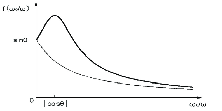
Figure 1: A sketch of $f\left(\frac{\omega_{0}}{\omega}\right)$. The solid line is for $\theta\in(0,\frac{\pi}{2}]$ and the dashed line is for $\theta\in(\frac{\pi}{2},\pi)$.

In the second case where $\theta\in(\frac{\pi}{2},\pi)$, $f(\frac{\omega_{0}}{\omega})$ is a monotonic decreasing function of $\frac{\omega_{0}}{\omega}$ in its domain. It is always larger than $\sin\frac{\theta}{2}$ in the interval $0<\frac{\omega_{0}}{\omega}\leq 1$. The dashed line in Fig. $1$ is a sketch of $f(\frac{\omega_{0}}{\omega})$ for $\theta\in(\frac{\pi}{2},\pi)$. These calculations show that for a nonzero $\sin\theta$, the adiabatic approximation is valid only if $\omega_{0}\gg\omega$, which necessarily implies the quantitative condition $\omega_{0}\gg\omega\sin\theta$. If $\omega_{0}\gg\omega$ is not fulfilled, for instance $\omega_{0}\ll\omega$ or $\omega_{0}\sim\omega$ , the absolute value of $b(t)$ in Eq. (23) is in the order of $\sin\theta$, and therefore the adiabatic approximation is invalid.

After having demonstrated that $\omega_{0}\gg\omega\sin\theta$ is a necessary condition for the adiabatic evolution of the spin-half system, we now explain what is wrong in the claim that the quantitative condition was unnecessary. It was argued that if $\sin\theta$ is small enough, the fidelity between $|\psi(t)\rangle$ and $|\psi^{adi}(t)\rangle$ will then be close to $1$ and the adiabatic approximation would be valid even if $\omega_{0}\ll\omega$. Certainly, it is true that the fidelity may be close to $1$ if $\sin\theta$ is small enough, but this does not imply that the adiabatic approximation is valid for $\omega_{0}\ll\omega$. In fact, $|\psi(t)\rangle$ cannot be expressed as $a(t)|E_{1}(t)\rangle$ if only $\sin\theta$ is small but not $\omega_{0}\gg\omega$. To clarify this point, let us rewrite Eq. (23) as $|\psi(t)\rangle=\left(\begin{array}[]{c}A_{1}+B_{1}\\ A_{2}+B_{2}\end{array}\right)$, where $A_{i}$ and $B_{i}$ are determined by $\left(\begin{array}[]{c}A_{1}\\ A_{2}\end{array}\right)\equiv a(t)|E_{1}(t)\rangle,~{}\left(\begin{array}[]{c}B_{1}\\ B_{2}\end{array}\right)\equiv b(t)|E_{2}(t)\rangle$. By using Eqs (19),(23) and (24), the explicit expressions of $A_{i}$ and $B_{i}$ can be obtained. One may find that $B_{2}$ relative to $A_{2}$ is much smaller, and it is valid to have $A_{2}+B_{2}\approx A_{2}$. Yet, $B_{1}$ is of the same order as $A_{1}$, and it is invalid to take $A_{1}+B_{1}\approx A_{1}$. Therefore, one cannot take $a(t)|E_{1}(t)\rangle$ as an approximation of $|\psi(t)\rangle$. Further more, we can also find the distinct difference between $|\psi(t)\rangle$ and $|\psi^{adi}(t)\rangle$ by comparing the Bloch vectors of them. The exact solution (23) can be explicitly written as

$$|\psi(t)\rangle=\left(\begin{array}[]{c}e^{-i\omega t/2}\sin\frac{\theta}{2}\left(\cos\frac{\overline{\omega}t}{2}+i\frac{\omega_{0}+\omega}{\overline{\omega}}\sin\frac{\overline{\omega}t}{2}\right)\\ -e^{i\omega t/2}\cos\frac{\theta}{2}\left(\cos\frac{\overline{\omega}t}{2}+i\frac{\omega_{0}-\omega}{\overline{\omega}}\sin\frac{\overline{\omega}t}{2}\right)\end{array}\right).$$ (28)

If $\omega_{0}\ll\omega$, we have $\frac{\omega_{0}\pm\omega}{\overline{\omega}}\approx\pm 1$ and $\overline{\omega}\approx\omega-\omega_{0}\cos\theta+\delta$, where $\delta=\delta(\frac{\omega_{0}}{\omega})$ is of the order $\frac{\omega_{0}}{\omega}$. Equation (28) then becomes

$$|\psi(t)\rangle\approx\left(\begin{array}[]{c}e^{-i(\omega_{0}\cos\theta-\delta)t/2}\sin\frac{\theta}{2}\\ -e^{i(\omega_{0}\cos\theta-\delta)t/2}\cos\frac{\theta}{2}\end{array}\right).$$ (31)

Clearly, the Bloch vector of $|\psi^{adi}(t)\rangle$ is rotating as fast as the magnetic field. However, from Eq. (31), we find that for the exact solution $|\psi(t)\rangle$, the rotating rate of its Bloch vector is about $\omega_{0}$, which is far from the rotating rate of the magnetic field. Therefore, if $\omega_{0}\ll\omega$, the system is never in the adiabatic evolution, no matter how small $\sin\theta$ is. For instance, if we take $\theta=0.06$ and $\omega=10\omega_{0}$, as in Ref. Du2008 , the rotating rate of the state $|\psi(t)\rangle$ is 10 times as much as that of $|\psi^{adi}(t)\rangle$ although the fidelity between the two states is close to $1$.

In summary, we have proved that the quantitative condition is necessary in guaranteeing the validity of the adiabatic approximation. One can then conclude that the quantitative condition is a necessary but insufficient one. Fulfilling only the quantitative condition may not guarantee the validity of the adiabatic approximation, but violating the condition must lead to the invalidity of the approximation. Since the quantitative condition plays an important role in the practical applications of the adiabatic theorem and it had been found to be insufficient, the confirmation of its necessity is of great importance. Besides, the findings in the letter have removed all the previous doubts or misunderstandings on the quantitative condition. In passing, we would like to point out that the quantitative condition may be a necessary and sufficient criterion of the adiabatic approximation for a large number of interesting quantum systems, although it is difficult to pick out these systems. This may be the underlying reason that the quantitative condition is still a powerful tool widely used by researchers despite the finding of its insufficiency.

D. M. Tong thanks G. L. Long and J. F. Du for useful discussions. This work was supported by NSF China with No.10875072 and the National Basic Research Program of China (Grant No. 2009CB929400).

References

- (1) M. Born and V. Fock, Z. Phys. 51, 165(1928).
- (2) J. Schwinger, Phys. Rev. 51, 648(1937).
- (3) L. I. Schiff, Quantum Mechanics (McGRAW-Hill Book Co., Inc., New York, 1949).
- (4) D. Bohm, Quantum Theory (Prentic-Hall, Inc., New York, 1951).
- (5) T. Kato, J. Phys. Soc. Jap. 5, 435 (1950).
- (6) A. Messiah, Quantum Mechanics (North-Holland Pub. Co., Amsterdam,1962).
- (7) L. D. Landau, Phys. Z. Sowjetunion 2, 46 (1932).
- (8) C. Zener, Proc. R. Soc. London A 137, 696 (1932).
- (9) M. Gell-Mann and F. Low, Phys. Rev. 84, 350 (1951).
- (10) M.V. Berry, Proc. R. Soc. London Ser. A 392, 45 (1984).
- (11) E. Farhi et al, Science 292, 472(2001).
- (12) K. P. Marzlin and B. C. Sanders, Phys. Rev. Lett. 93, 160408 (2004).
- (13) D. M. Tong, K. Singh, L. C. Kwek, and C. H. Oh, Phys. Rev. Lett. 95, 110407 (2005).
- (14) T. Vertesi, R. Englman, Phys. Lett. A 353, 11 (2006).
- (15) S. Duki, H. Mathur, O. Narayan, Phys. Rev. Lett. 97, 128901 (2006).
- (16) J. Ma, Y. P. Zhang, E. G. Wang, B. Wu, Phys. Rev. Lett. 97, 128902 (2006).
- (17) M. Y. Ye, X. F. Zhou, Y. S. Zhang et al., Phys. Lett. A 368, 18 (2007).
- (18) R. MacKenzie, A. Morin-Duchesne, H. Paquette,J. Pinel/, Phys. Rev. A 76, 044102 (2007).
- (19) Y. Zhao, Phys. Rev. A 77, 032109 (2008).
- (20) J. F. Du, L. Z. Hu, Y. Wang et al., Phys. Rev. Lett. 101, 060403 (2008).
- (21) M. H. S. Amin, Phys. Rev. Lett. 102, 220401 (2009).
- (22) R. MacKenzie, E. Marcotte, H. Paquette, Phys. Rev. A 73, 042104 (2006).
- (23) D. M. Tong, K. Singh, L. C. Kwek, C. H. Oh, Phys. Rev. Lett. 98, 150402 (2007).
- (24) Z. H. Wei, M.S. Ying, Phys. Rev. A 76, 024304 (2007).
- (25) S. Jansen, M. B.Ruskai, R. Seiler, J. Math. Phys. 48, 102111 (2007).
- (26) K. Fujikawa, Phys. Rev. D 77, 045006 (2008).
- (27) J. D. Wu, M .S. Zhao, J. L. Chen, Y. D. Zhang, Phys. Rev. A 77, 062114 (2008).
- (28) M. Maamache, Y. Saadi, Phys. Rev. Lett. 101, 150407 (2008).
- (29) G. Rigolin, G. Ortiz, V. H. Ponce, Phys. Rev. A 78, 052508 (2008).
- (30) V. I. Yukalov, Phys. Rev. A 79, 052117 (2009).
- (31) D. Comparat, Phys. Rev. A 80, 012106 (2009).
- (32) X. L. Huang, X. X. Yi, Phys. Rev. A 80, 032108 (2009).
- (33) D. A. Lidar, A. T. Rezakhani, A. Hamma, J Math. Phys. 50, 102106 (2009).
- (34) J. Larson and S. Stenholm , Phys. Rev. A 73, 033805 (2006).
- (35) J. Liu and L. B. Fu, Phys. Lett. A 370, 17 (2007).
- (36) K. Y. Bliokh, Phys. Lett. A 372, 204 (2008).
- (37) D. M. Tong, X. X. Yi et al., Phys. Lett. A 372, 2364 (2008).
- (38) M. J. O’Hara and D. P. O’Leary, Phys. Rev. A 77, 042319 (2008).
- (39) T. Barthel, C. Kasztelan, I. P. McCulloch, U. Schollwock/, Phys. Rev. A 79, 053627 (2009).
- (40) S. J. Gu, Phys. Rev. E 79, 061125 (2009).