Current Observational Constraints to Holographic Dark Energy Model with New Infrared cut-off via Markov Chain Monte Carlo Method

Abstract

In this paper, the holographic dark energy model with new infrared (IR) cut-off for both the flat case and the non-flat case are confronted with the combined constraints of current cosmological observations: type Ia Supernovae, Baryon Acoustic Oscillations, current Cosmic Microwave Background, and the observational hubble data. By utilizing the Markov Chain Monte Carlo (MCMC) method, we obtain the best fit values of the parameters with $1\sigma,2\sigma$ errors in the flat model: $\Omega_{b}h^{2}=0.0233^{+0.0009+0.0013}_{-0.0009-0.0014}$, $\alpha=0.8502^{+0.0984+0.1299}_{-0.0875-0.1064}$, $\beta=0.4817^{+0.0842+0.1176}_{-0.0773-0.0955}$, $\Omega_{de0}=0.7287^{+0.0296+0.0432}_{-0.0294-0.0429}$, $\Omega_{m0}=0.2713^{+0.0294+0.0429}_{-0.0296-0.0432}$, $H_{0}=66.35^{+2.38+3.35}_{-2.14-3.07}$. In the non-flat model, the constraint results are found in $1\sigma,2\sigma$ regions: $\Omega_{b}h^{2}=0.0228^{+0.0010+0.0014}_{-0.0010-0.0014}$, $\Omega_{k}=0.0305^{+0.0092+0.0140}_{-0.0134-0.0176}$, $\alpha=0.8824^{+0.2180+0.2213}_{-0.1163-0.1378}$, $\beta=0.5016^{+0.0973+0.1247}_{-0.0871-0.1102}$, $\Omega_{de0}=0.6934^{+0.0364+0.0495}_{-0.0304-0.0413}$, $\Omega_{m0}=0.2762^{+0.0278+0.0402}_{-0.0320-0.0412}$, $H_{0}=70.20^{+3.03+3.58}_{-3.17-4.00}$. In the best fit holographic dark energy models, the equation of state of dark energy and the deceleration parameter at present are characterized by $w_{de0}=-1.1414\pm 0.0608,q_{0}=-0.7476\pm 0.0466$ (flat case) and $w_{de0}=-1.0653\pm 0.0661,q_{0}=-0.6231\pm 0.0569$ (non-flat case). Compared to the $\Lambda\textmd{CDM}$ model, it is found the current combined datasets do not favor the holographic dark energy model over the $\Lambda\textmd{CDM}$ model.

I Introduction

Since 1998, the type Ia supernova (SNe Ia) observations ref:Riess98 ; ref:Perlmuter99 have shown that our universe has entered into a phase of accelerating expansion. During these years from that time, many additional observational results, including current Cosmic Microwave Background (CMB) anisotropy measurement from Wilkinson Microwave Anisotropy Probe (WMAP)ref:Spergel03 ; ref:Spergel06 , and the data of the Large Scale Structure (LSS) from Sloan Digital Sky Survey (SDSS) ref:Tegmark1 ; ref:Tegmark2 , also strongly support this suggestion. These observational results have greatly inspirited theorists to understand the mechanism of the accelerating expansion of the universe, which is usually attributed to an exotic energy component with negative pressure, dubbed dark energy (DE). The simplest but most natural candidate of DE is the cosmological constant $\Lambda$, with the constant equation of state (EOS) $w=-1$. As we know, the cosmic concordance model confronts with two difficulties: the fine-tuning problem and the cosmic coincidence problem. Both of these problems are related to the DE density. In order to solve or alleviate cosmological constant puzzles, many dynamical DE models are proposed, where the DE density and its EOS are time-varying. However, the predictions of the cosmological constant model still fit to the current observations ref:LCDM1 ; ref:LCDM2 ; ref:LCDM3 . Therefore the dynamical DE models being proposed should not be far away from the cosmological constant model, such as quintessence ref:quintessence01 ; ref:quintessence02 ; ref:quintessence1 ; ref:quintessence2 ; ref:quintessence3 ; ref:quintessence4 , phantom ref:phantom , quintom ref:quintom , K-essence ref:kessence , tachyon ref:tachyon , ghost condensate ref:ggc , holographic DE ref:holo1 ; ref:holo2 and agegraphic DE ref:age1 ; ref:age2 etc. Although many DE models have been presented, the nature of DE is still a conundrum. This puzzle can not be understood before a complete theory of quantum gravity is established. But the two additional aspects from the current cosmological observations and some basic quantum gravitational principles may shed light on probing the nature of DE.

On the one hand, provided that we know little on the theoretical nature of DE at present, the combined cosmic observations can play an important role in understanding the nature of DE. The cosmological parameters space in the DE model can be determined by the constraints of the data combinations. Recently, the 397 SN Ia data was compiled in Ref. ref:Condata by adding CfA3 sample from the CfA SN Group to the Union set by Ref. ref:Kowalski , which include 250 SN Ia at high redshift but only 57 at low redshift, to form the Constitution set. Aside from the SN Ia data, the combined analysis is required in order to break the degeneracy between the cosmological parameters, which includes cosmic observations from baryon acoustic oscillations (BAO), CMB and the observational Hubble data (OHD). The BAO are detected in the clustering of the combined 2dFGRS and SDSS main galaxy samples or the SDSS luminous red galaxies and measure the distance-redshift relation. From these samples, the values of $[r_{s}(z_{d})/D_{V}(0.2),r_{s}(z_{d})/D_{V}(0.35)]$ and their inverse covariance matrix in the measurement of BAO can be obtained ref:Percival2 . For the measurement of CMB, we utilize the shift parameter $R$ at the photon decoupling epoch $z_{\ast}$, the acoustic scale $l_{A}(z_{\ast})$, and together with the physical baryon density parameter multiplied by 100, thus it is $100\Omega_{b}h^{2}$ ref:Komatsu2008 ; ref:Bueno Sanchez . Here, it is worth noting that the WMAP distance information $R(z_{\ast})$ and $l_{A}(z_{\ast})$ can not be measured by WMAP directly, but are derived from making a global fitting constraint with MCMC method by using the full WMAP data on the assumption that a certain cosmological model has been given in advance ref:lAR . Although in theory the inverse covariance matrix on $R(z_{\ast})$ and $l_{A}(z_{\ast})$ is model dependent, it is feasible to use the derived results about $R(z_{\ast})$ and $l_{A}(z_{\ast})$ to constrain the parameters in another DE model since $R(z_{\ast})$ and $l_{A}(z_{\ast})$ do not depend strongly on the DE model which is not far away from the cosmological constant model ref:lAR . What is more, the paper ref:ywang has been demonstrated that $[R(z_{\ast}),l_{A}(z_{\ast}),100\Omega_{b}h^{2}]$ effectively provide a good summary of CMB data when the DE model parameters are constrained. In addition, we employ the OHD at twelve different redshifts determined by using the differential ages of passively evolving galaxies in Ref. ref:0907 , where the value of the Hubble constant is replaced by $H_{0}=74.2\pm 3.6$ in Ref. ref:0905 , and add the three more observational data $H(z=0.24)=79.69\pm 2.32,H(z=0.34)=83.8\pm 2.96,$ and $H(z=0.43)=86.45\pm 3.27$ in ref:0807 . Since the constraint results of a given model are dependent on the combined data ref:Gdata ; ref:XUdata , in this paper we use a fully combined observations from the 397 SN Ia standard candle data, the value of $[r_{s}(z_{d})/D_{V}(0.2),r_{s}(z_{d})/D_{V}(0.35)]$ and their inverse covariance matrix in the measurement of BAO, the values of $[R(z_{\ast}),l_{A}(z_{\ast}),100\Omega_{b}h^{2}]$ and their inverse covariance matrix in the measurement of CMB, and the fifteen OHD.

On the other hand, the models which are constructed in light of some fundamental principle are more charming, since this kind of DE model may exhibit some underlying features of DE, for instance the holographic DE model ref:holo1 ; ref:holo2 and the agegraphic DE model ref:age1 ; ref:age2 . The holographic DE model is built on the basis of holographic principle and some features of quantum gravity theory. The agegraphic DE model is derived from taking the combination between the uncertainty relation in quantum mechanics and general relativity into account. In this paper, we focus on the holographic DE model, which is considered as a dynamic vacuum energy. According to the holographic principle, the number of degrees of freedom in a bounded system should be finite and is related to the area of its boundary. By applying the principle to cosmology, one can obtain the upper bound of the entropy contained in the universe. For a system with size $L$ and UV cut-off $\Lambda$ without decaying into a black hole, it is required that the total energy in a region of size $L$ should not exceed the mass of a black hole of the same size, thus $L^{3}\rho_{\Lambda}\leq LM_{pl}^{2}$. The largest $L$ allowed is the one saturating this inequality, thus we obtain the holographic DE density

$$\rho_{\Lambda}=\frac{3c^{2}M_{pl}^{2}}{L^{2}},$$ (1)

where c is a numerical constant and $M_{pl}$ is the reduced Planck Mass $M_{pl}\equiv 1/\sqrt{8\pi G}$. It just means a duality between UV cut-off and IR cut-off. The UV cut-off is related to the vacuum energy, and IR cut-off is related to the large scale of the universe, for example Hubble horizon, particle horizon, event horizon, Ricci scalar or the generalized functions of dimensionless variables as discussed by ref:holo1 ; ref:holo2 ; ref:holo3 ; ref:EPJCXU . Next, we give a brief review on the main results when Hubble horizon, particle horizon, event horizon or Ricci scalar are taken as the IR cut-off, respectively.

$\bullet$ $L^{-2}=H^{2}$. As pointed in ref:holo2 , it is found that the holographic DE density is in proportion to $H^{2}$, the same as dark matter density, i.e. $\rho_{de}/c^{2}=\rho_{m}/(1-c^{2})\propto H^{2}$. It appears that it is natural to solve the coincidence problem. However, Hsu ref:holo1 pointed out that the dark energy EOS $w_{de}=0$ was obtained in this instance. It is obvious that this result is not consistent with the current observations. This bad situation can be changed by considering the holographic DE with Hubble horizon as the time variable cosmological constant. More detailed analysis is presented in Ref. ref:XU071709 .

$\bullet$ $L^{-2}=R_{ph}(a)=a\int_{0}^{t}\frac{dt^{\prime}}{a(t^{\prime})}=a\int_{0}^{a}\frac{da^{\prime}}{Ha^{\prime 2}}$. As shown in paper ref:holo2 , Li pointed out that this yields the dark energy EOS is not less than $-1/3$. Thus the current accelerated expansion of our universe can not be well explained. However, this result in ref:holo2 is obtained on the assumption that DE dominates. The holographic DE model with particle horizon has been discussed in detail by ref:XU054772 .

$\bullet$ $L^{-2}=R_{eh}(a)=a\int_{t}^{\infty}\frac{dt^{\prime}}{a(t^{\prime})}=a\int_{a}^{\infty}\frac{da^{\prime}}{Ha^{\prime 2}}$. The holographic DE model with event horizon can reveal the dynamic nature of the vacuum energy and provide a desired EOS of the holographic DE with the model parameter $c$. Furthermore, the holographic DE behaves like quintessence, cosmological constant and phantom respectively for the different values of the model parameter: $c\geq 1$, $c=1$ and $c\leq 1$ ref:holo2 . Therefore, the value of model parameter $c$ plays a crucial role in determining the property of holographic DE in this case. However, this model is confronted with the causality problem: why should the present density of DE be determined by the future event horizon of the universe.

$\bullet$ $L^{-2}=R=-6(\dot{H}+2H^{2}+\frac{k}{a^{2}})$. In ref:holo3 , it has shown that this model can avoid the causality problem and naturally solve the coincidence problem of dark energy after Ricci scalar is taken as the IR cut-off and the parameters have been well constrained by the combined astronomical observations ref:MPLAXU ; ref:LiRicci .

Subsequently, In ref:holo4 , Granda and Oliveros generalized the form of the IR cut-off on the basis of the Ricci scalar:

$$L^{-2}=\alpha H^{2}+\beta\dot{H},$$ (2)

where there are two independent model parameters $\alpha$ and $\beta$, which can be determined by using the combined constraints of the thorough observational datasets. In this paper, we consider the holographic DE model with new IR cut-off in both flat and non-flat case. The performance of a global fitting will be made by using the Markov Chain Monte Carlo (MCMC) method. In this way, we can work in the framework of multi-parameter freedoms, including the basic cosmological parameters ($\Omega_{b}h^{2},\Omega_{c}h^{2},\Omega_{k}$) and the new-added model parameters ($\alpha,\beta$).

The paper is organized as follows. In next section, we briefly review the holographic DE model with new IR cut-off. In section III, we perform the cosmic observation constraint on the holographic DE model. The last section is the conclusion.

II Review of Holographic Dark Energy Model with New Infrared cut-off

In this section, we give a brief review on the general formula in the holographic DE model with new IR cut-off. With a Friedmann-Robertson-Walker (FRW) metric

$$ds^{2}=-dt^{2}+a^{2}(t)[\frac{dr^{2}}{1-kr^{2}}+r^{2}(d{\theta}^{2}+\sin^{2}{\theta}d{\phi}^{2})],$$ (3)

the Einstein field equation can be written as

$$H^{2}=\frac{1}{3M_{pl}^{2}}\sum_{i}\rho_{i},$$ (4)

$$\frac{\ddot{a}}{a}=-\frac{1}{6M_{pl}^{2}}\sum_{i}(\rho_{i}+3P_{i}),$$ (5)

where $H$ is the Hubble function, and $\rho_{i}$ and $P_{i}$ are the energy density and the pressure of a general piece of matter, and their subscripts $i$ denote $m$, $de$ and $k$, which respectively correspond to matter component, the holographic DE with new infrared cut-off and the curvature part of space. Here the matter component includes the cold dark matter and the baryon matter, i.e.

$$\rho_{m}=\rho_{cdm}+\rho_{b},P_{m}=0.$$ (6)

The parameter $k=1,0,-1$ denote the closed, flat and open geometries, respectively. The effective energy density and the effective pressure of the curvature part are

$$\rho_{k}=-\frac{3M_{pl}^{2}k}{a^{2}},$$ (7)

$$P_{k}=-\rho_{k}-\frac{\dot{\rho}_{k}}{3H}.$$ (8)

As suggested by Granda and Oliveros in paper ref:holo4 , the energy density of the holographic DE with new IR cut-off is given as

$$\rho_{de}=3M_{pl}^{2}(\alpha H^{2}+\beta\dot{H}),$$ (9)

where $\alpha$ and $\beta$ are the dimensionless parameters in holographic DE model with new IR cut-off, which are regarded as independent of each other. In this paper, a dot denotes a derivative with respect to the cosmic time $t$. After changing the variable from the cosmic time $t$ to $x=\ln a$, we can rewritten the Eq. (4) as

$$H^{2}=\frac{1}{3M_{pl}^{2}}\rho_{m0}e^{-3x}-ke^{-2x}+\alpha H^{2}+\frac{1}{2}\beta\frac{dH^{2}}{dx}.$$ (10)

With the help of the definitions as follows:

$$E=\frac{H}{H_{0}},\Omega_{m0}=\frac{\rho_{m0}}{3M_{pl}^{2}H_{0}^{2}},\Omega_{k}=-\frac{k}{H_{0}^{2}},$$ (11)

the Eq. (10) can be ulteriorly rewritten as

$$E^{2}=\Omega_{k}e^{-2x}+\Omega_{m0}e^{-3x}+\alpha E^{2}+\frac{1}{2}\beta\frac{dE^{2}}{dx}.$$ (12)

Solving this first order differential equation about $E^{2}$, we can obtain

$$E^{2} = \Omega_{k}e^{-2x}+\Omega_{m0}e^{-3x}+\frac{2\alpha-3\beta}{3\beta-2\alpha+2}\Omega_{m0}e^{-3x}+\frac{\alpha-\beta}{\beta-\alpha+1}\Omega_{k}e^{-2x}+f_{0}e^{-\frac{2(\alpha-1)}{\beta}x}$$ (13)

$$= \Omega_{k}e^{-2x}+\Omega_{m0}e^{-3x}+\Omega_{de}(x),$$

where $f_{0}$ is the integral constant and can be derived from the initial condition $E_{0}=1$, which is $f_{0}=1-\frac{1}{\beta-\alpha+1}\Omega_{k}-\frac{2}{3\beta-2\alpha+2}\Omega_{m0}$, and $\Omega_{de}(x)$ is the dimensionless energy density of the holographic DE with new IR cut-off:

$$\Omega_{de}(x)=\frac{2\alpha-3\beta}{3\beta-2\alpha+2}\Omega_{m0}e^{-3x}+\frac{\alpha-\beta}{\beta-\alpha+1}\Omega_{k}e^{-2x}+(1-\frac{1}{\beta-\alpha+1}\Omega_{k}-\frac{2}{3\beta-2\alpha+2}\Omega_{m0})e^{-\frac{2(\alpha-1)}{\beta}x},$$ (14)

Then, combining the above definition of the dimensionless energy density of the holographic DE with its conservation equation, we can obtain the EOS of the holographic DE with new IR cut-off

$$w_{de}(z)=-1+\frac{1+z}{3}\frac{d\ln{\Omega_{de}}}{dz}.$$ (15)

In addition, we shall investigate the evolution of the deceleration parameter. Combining Eqs. (4) and (5) with the definition of the deceleration parameter, we can get

$$q(z) {=}\frac{1}{2}+\frac{3}{2}\frac{\sum_{i}\tilde{P_{i}}}{\sum_{i}\tilde{\rho_{i}}}$$ (16)

$${=}\frac{1}{2}+\frac{3}{2}\frac{\sum_{i}\tilde{P_{i}}}{\Omega_{m0}(1+z)^{3}+\Omega_{k}(1+z)^{2}+\Omega_{de}(z)},$$

where we have utilized the definitions of $\tilde{P_{i}}=\frac{P_{i}}{3M_{pl}^{2}H_{0}^{2}}$ and $\tilde{\rho_{i}}=\frac{\rho_{i}}{3M_{pl}^{2}H_{0}^{2}}$. According to the energy conservation equation, we have

$$\tilde{P_{i}}=-\tilde{\rho_{i}}-\frac{1}{3}\frac{d\tilde{\rho_{i}}}{dx}.$$ (17)

In the review above, it is direct and natural to consider the parameters $\beta\neq 0$ and $\alpha\neq 1$ when we solve the differential Eq. (12). Next, we discuss three special cases when the denominators in Eq. (13) equal zero as follows:

Case 1: $3\beta-2\alpha+2=0$ and $\beta-\alpha+1=0$

In this case, we obtain $\beta=0$ and $\alpha=1$. Now the energy density of the holographic DE is $\rho_{de}=3M_{pl}^{2}H^{2}$. Compared to the Friedmann equation, it is found that the DE density is not consistent with the current observations of $70\%$ exotic component in the universe.

Case 2: $3\beta-2\alpha+2\neq 0$ and $\beta-\alpha+1=0$

From the latter equation, we can get $\beta=\alpha-1$. Then the energy density of the holographic DE is $\rho_{de}=3M_{pl}^{2}(\frac{\alpha-1}{2}\frac{dH^{2}}{dx}+\alpha H^{2})$. In this case, the solution of the first order differential equation is

$$E^{2} {=}f_{0}e^{-2x}+\frac{2}{\alpha-1}\Omega_{m0}e^{-3x}-\frac{2}{\alpha-1}x\Omega_{k}e^{-2x}$$ (18)

$${=}\Omega_{k}e^{-2x}+\Omega_{m0}e^{-3x}+\Omega_{de}(x),$$

where we have set the integral constant $f_{0}=\Omega_{k}$ and defined $\Omega_{de}(x)=\frac{3-\alpha}{\alpha-1}\Omega_{m0}e^{-3x}-\frac{2}{\alpha-1}x\Omega_{k}e^{-2x}$ as the dimensionless energy density of the holographic DE. Considering the current value of the dimensionless DE density, we can obtain the value of the only model parameter $\alpha=\frac{3\Omega_{m0}+\Omega_{de0}}{\Omega_{m0}+\Omega_{de0}}$. So the case is a viable DE model.

Case 3: $3\beta-2\alpha+2=0$ and $\beta-\alpha+1\neq 0$

From the former equation, we can obtain $\beta=\frac{2(\alpha-1)}{3}$. Then the energy density of the holographic DE is $\rho_{de}=3M_{pl}^{2}(\frac{\alpha-1}{3}\frac{dH^{2}}{dx}+\alpha H^{2})$. In this case, the solution of the first order differential equation is

$$E^{2} {=}f_{0}e^{-3x}-\frac{3}{\alpha-1}x\Omega_{m0}e^{-3x}-\frac{3}{\alpha-1}\Omega_{k}e^{-2x}$$ (19)

$${=}\Omega_{m0}e^{-3x}+\Omega_{k}e^{-2x}+\Omega_{de}(x),$$

where we have taken the integral constant $f_{0}=\Omega_{m0}$ and defined $\Omega_{de}(x)=-\frac{3}{\alpha-1}x\Omega_{m0}e^{-3x}-\frac{2+\alpha}{\alpha-1}\Omega_{k}e^{-2x}$ as the dimensionless energy density of the holographic DE. Considering the current value of the dimensionless DE density, we can get the value of the only model parameter $\alpha=\frac{\Omega_{de0}-2\Omega_{k}}{\Omega_{de0}+\Omega_{k}}$. So the case with the non-flat background geometry is a viable dark energy model. The result in the flat case is the same as Case 1.

As far as the Case 2 and Case 3 discussed above are concerned, the model parameters $\alpha$ and $\beta$ are reliant on each other. In this paper, we consider the generalized case with independent model parameters. In the next section, according to the combined observational data, we restrict the basic cosmological parameters and the model parameters, all of which are independent on each other.

III Method and results

parameters		flat holographic		not-flat holographic		flat $\Lambda\textmd{CDM}$		not-flat $\Lambda\textmd{CDM}$
$\Omega_{b}h^{2}$		$0.0233^{+0.0009+0.0013}_{-0.0009-0.0014}$		$0.0228^{+0.0010+0.0014}_{-0.0010-0.0014}$		$0.0228^{+0.0007+0.0011}_{-0.0007-0.0011}$		$0.0228^{+0.0007+0.0011}_{-0.0008-0.0013}$
$\Omega_{k}$		-		$0.0305^{+0.0092+0.0140}_{-0.0134-0.0176}$		-		$-0.0013^{+0.0070+0.0103}_{-0.0076-0.0108}$
$\alpha$		$0.8502^{+0.0984+0.1299}_{-0.0875-0.1064}$		$0.8824^{+0.2180+0.2213}_{-0.1163-0.1378}$		-		-
$\beta$		$0.4817^{+0.0842+0.1176}_{-0.0773-0.0955}$		$0.5016^{+0.0973+0.1247}_{-0.0871-0.1102}$		-		-
$\Omega_{de0}/\Omega_{\Lambda 0}$		$0.7287^{+0.0296+0.0432}_{-0.0294-0.0429}$		$0.6934^{+0.0364+0.0495}_{-0.0304-0.0413}$		$0.7220^{+0.0177+0.0273}_{-0.0185-0.0315}$		$0.7258^{+0.0222+0.0317}_{-0.0268-0.0407}$
$\Omega_{m0}$		$0.2713^{+0.0294+0.0429}_{-0.0296-0.0432}$		$0.2762^{+0.0278+0.0402}_{-0.0320-0.0412}$		$0.2780^{+0.0185+0.0315}_{-0.0177-0.0273}$		$0.2755^{+0.0239+0.0367}_{-0.0186-0.0274}$
$H_{0}$		$66.35^{+2.38+3.35}_{-2.14-3.07}$		$70.20^{+3.03+3.58}_{-3.17-4.00}$		$70.11^{+1.44+2.35}_{-1.34-2.24}$		$70.04^{+1.72+2.81}_{-2.20-2.91}$
$\chi^{2}/dof$		$1.23849$		$1.15996$		$1.15339$		$1.15589$

Table 1: The data fitting results of the cosmological parameters and the model parameters with $1\sigma$, $2\sigma$ regions in the flat and non-flat holographic DE model with new infrared cut-off and $\Lambda\textmd{CDM}$ model (flat case and non-flat case), where the combined observational data from SN $397$, BAO and CMB and OHD are used.

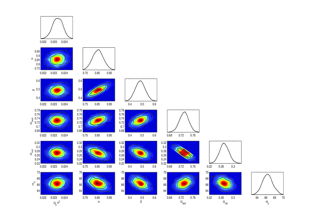
Figure 1: 1-D constraints on individual parameters ($\Omega_{b}h^{2},\alpha,\beta,\Omega_{de0},\Omega_{m0},H_{0}$) and 2-D contours on these parameters with $1\sigma,2\sigma$ errors between each other using the combination of the observational data from SN $397$, BAO, CMB and OHD in the flat holographic DE model with new IR cut-off. Dotted lines in the 1-D plots show the mean likelihood of the samples and the solid lines are marginalized probabilities for the parameters in the flat holographic DE model with new IR cut-off ref:MCMC .

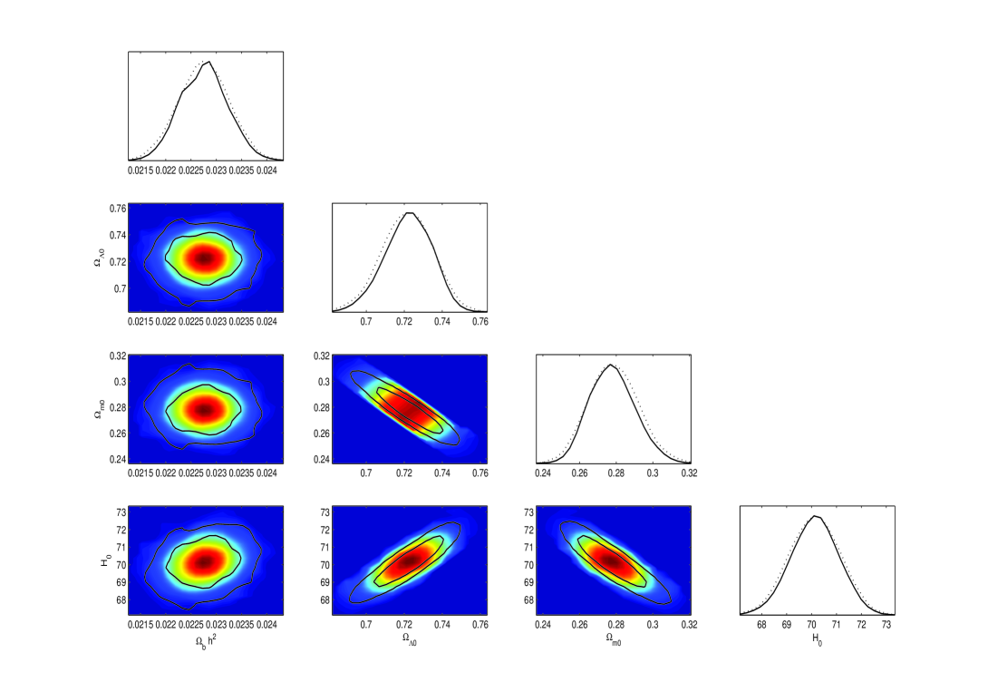
Figure 2: 1-D constraints on individual parameters ($\Omega_{b}h^{2},\Omega_{\Lambda 0},\Omega_{m0},H_{0}$) and 2-D contours on these parameters with $1\sigma,2\sigma$ errors between each other using the combination of the observational data from SN $397$, BAO, CMB and OHD in the flat $\Lambda\textmd{CDM}$ model. Dotted lines in the 1-D plots show the mean likelihood of the samples and the solid lines are marginalized probabilities for the parameters in the flat $\Lambda\textmd{CDM}$ model ref:MCMC .

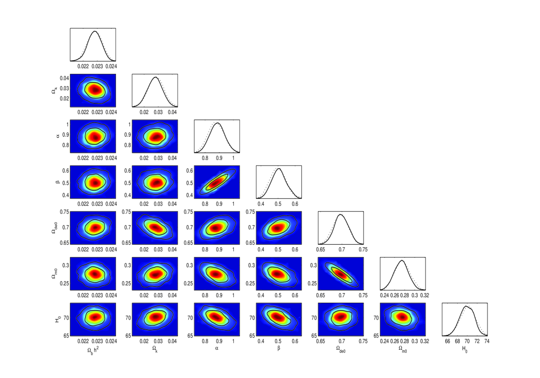
Figure 3: 1-D constraints on individual parameters ($\Omega_{b}h^{2},\Omega_{k},\alpha,\beta,\Omega_{de0},\Omega_{m0},H_{0}$) and 2-D contours on these parameters with $1\sigma,2\sigma$ errors between each other using the combination of the observational data from SN $397$, BAO, CMB and OHD in the non-flat holographic DE model with new IR cut-off. Dotted lines in the 1-D plots show the mean likelihood of the samples and the solid lines are marginalized probabilities for the parameters in the non-flat holographic DE model with new IR cut-off ref:MCMC .

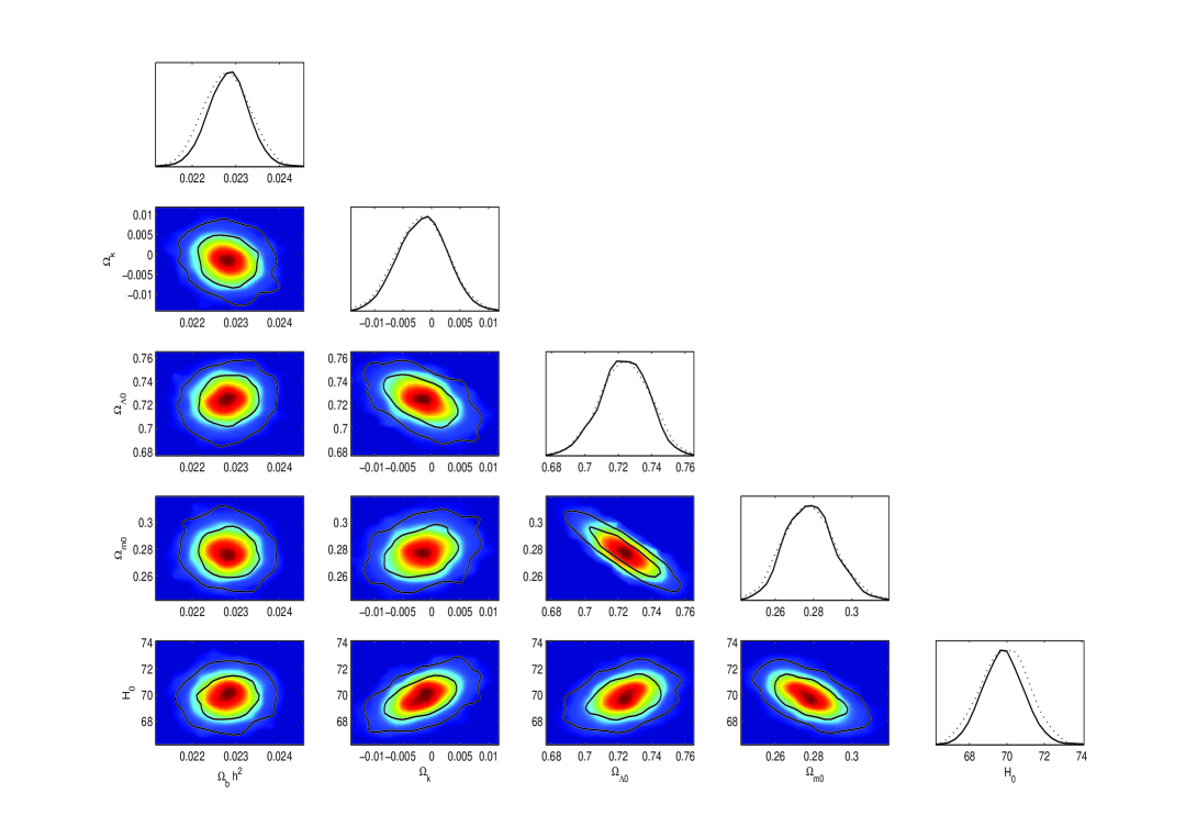
Figure 4: 1-D constraints on individual parameters ($\Omega_{b}h^{2},\Omega_{k},\Omega_{\Lambda 0},\Omega_{m0},H_{0}$) and 2-D contours on these parameters with $1\sigma,2\sigma$ errors between each other using the combination of the observational data from SN $397$, BAO, CMB and OHD in the non-flat $\Lambda\textmd{CDM}$ model. Dotted lines in the 1-D plots show the mean likelihood of the samples and the solid lines are marginalized probabilities for the parameters in the non-flat $\Lambda\textmd{CDM}$ model ref:MCMC .

In this section, we present the method and the data we have used. In our analysis, we perform a global fitting on determining the cosmological parameters using the Markov Chain Monte Carlo (MCMC) method. Since the computational requirements of MCMC procedures are insensitive to the dimensionality of the parameter space, we can expand the dimension of the parameter series, comparing with the traditional Maximum Likelihood (ML) method. The MCMC method is based on the publicly available CosmoMC package ref:MCMC , which has been modified to include the new parameters $\alpha$ and $\beta$ with having taken the weak priors as $\alpha\in[0.5,1.5]$ and $\beta\in[0.1,1.0]$. Besides the two independent model parameters, the basic cosmological parameters are also varying with top-hat priors: the physical baryon density $\Omega_{b}h^{2}\in[0.005,0.9]$, the dark matter energy density $\Omega_{c}h^{2}\in[0.01,0.99]$, and in the non-flat case, the additional parameter $\Omega_{k}\in[-0.1,0.1]$. In addition, we obtain three derived parameters $\Omega_{de0}$, $\Omega_{m0}$ and the Hubble constant $H_{0}$ from the basic cosmological parameters.

In our calculations, we have taken the total likelihood $L\propto e^{-\chi^{2}/2}$ to be the product of the separate likelihoods of SN, BAO, CMB and OHD. Then the $\chi^{2}$ is

$$\chi^{2}=\chi^{2}_{SN}+\chi^{2}_{BAO}+\chi^{2}_{CMB}+\chi^{2}_{OHD}.$$ (20)

The expressions of $\chi^{2}$s and datasets used in our paper are presented in Appendix A.

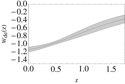
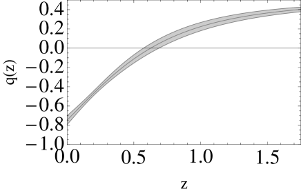
Figure 5: The evolutions of the EOS (the left panel) and the deceleration parameter (the right panel) in the flat holographic DE model with new IR cut-off with respect to the redshift $z$, where we have used the best fittings of the cosmological parameters and model parameters with $1\sigma$ errors.

The best fit values of the cosmological parameters and the model parameters with $1\sigma,2\sigma$ errors in holographic DE model with new IR cut-off and the $\Lambda\textmd{CDM}$ model for the flat case and the non-flat case are listed in Table 1. We calculate the values of $\chi^{2}/dof$, where $dof$ is the compact notation of the number of degrees of freedom and equals the number of observational data points minus the number of free parameters. It is found that the values of $\chi^{2}/dof$ exhibit a significant difference between the flat case and the non-flat case in the holographic DE model with the new IR cut-off. In this two instances, it is seen that the non-flat holographic DE model with a smaller value of $\chi^{2}/dof$ is much supported by the current observations. Subsequently, comparing the value of $\chi^{2}/dof$ in the non-flat holographic DE model with those in the $\Lambda$CDM models, we find the differences are not obvious. From the minor differences among the values of $\chi^{2}/dof$, we can conclude that the current combined datasets do not really favor the holographic DE model with the new IR cut-off over the concordance model. It is seen that the current observations support the flat concordance model with the smallest value of $\chi^{2}/dof$ the best. In Fig. 1, 2, we show one dimensional probability distribution of each parameter and two dimensional plots for parameters between each other in the flat holographic DE model with new IR cut-off and the flat $\Lambda\textmd{CDM}$ model. The corresponding plots in the non-flat holographic DE model with new IR cut-off and the non-flat $\Lambda\textmd{CDM}$ model are presented in Fig. 3,4.

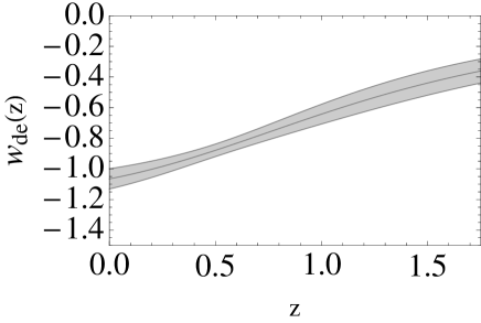
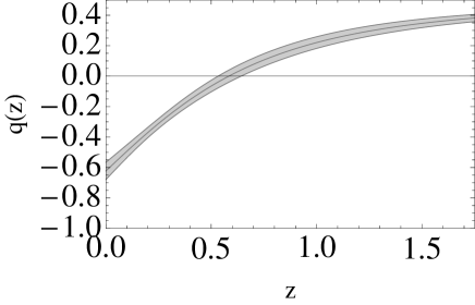
Figure 6: The evolutions of the EOS (the left panel) and the deceleration parameter (the right panel) in the non-flat holographic DE model with new IR cut-off with respect to the redshift $z$, where we have used the best fittings of the cosmological parameters and model parameters with $1\sigma$ errors.

Then, we investigate the evolutions of dark energy EOS and deceleration parameter in the holographic DE model. We consider the propagation of the errors for $w(z)$ and $q(z)$ by the Fisher matrix analysis. The errors are evaluated by using the covariance matrix $C_{ij}$ of the fitting parameters ref:wqerror1 ; ref:wqerror2 , which is the inverse of the Fisher matrix and given by

$$(C_{ij})^{-1}=-\frac{\partial^{2}\ln L}{\partial\theta_{i}\partial\theta_{j}},$$ (21)

where $\theta$ is a set of parameters, and $\ln L$ is the logarithmic likelihood function. The errors on a function $f=f(\theta)$ in terms of the variables $\theta$ are given by ref:wqerror2 ; ref:wqerror3

$$\sigma_{f}^{2}=\sum_{i}^{n}\left(\frac{\partial f}{\partial\theta_{i}}\right)^{2}C_{ii}+2\sum_{i}^{n}\sum_{j=i+1}^{n}\left(\frac{\partial f}{\partial\theta_{i}}\right)\left(\frac{\partial f}{\partial\theta_{j}}\right)C_{ij},$$ (22)

where $n$ is the number of parameters. Here, $f$ will be dark energy EOS $w(z;\theta_{i})$ or deceleration parameter $q(z;\theta_{i})$. The parameters $\theta_{i}$ respectively represent ($\Omega_{c}h^{2},\Omega_{b}h^{2},\alpha,\beta$) for the flat case and ($\Omega_{c}h^{2},\Omega_{b}h^{2},\Omega_{k},\alpha,\beta$) for the non-flat case. As shown in Fig. 5 (flat case) and Fig. 6 (non-flat case), we plot the evolutions of $w(z)$ and $q(z)$ with errors by

$$w_{1\sigma}(z)=w(z)|_{\theta=\bar{\theta}}\pm\sigma_{w},$$ (23)

$$q_{1\sigma}(z)=q(z)|_{\theta=\bar{\theta}}\pm\sigma_{q},$$ (24)

where $\bar{\theta}$ are the best fit values of the constraint parameters.

In Fig. 5 and Fig. 6, it is found that the combined observational data provide a fairly tight constraint on the holographic DE model with new IR cut-off. From the left panel in Fig. 5, it is seen that the EOS $w_{de}(z)$ with the best fit values can cross the boundary $-1$ and its current value is $w_{de}(z=0)=-0.1414$. From the right panel in Fig. 5, the value of the current deceleration parameter is given by $q_{0}=-0.7476\pm 0.0466$. In Fig. 6, we get the current value of the dark energy EOS in the non-flat case is $w_{de}(z=0)=-1.0653<-1$, i.e. it is also phantom-like. The present value of the deceleration parameter is $q_{0}=-0.6231\pm 0.0569$.

IV Conclusion

In summary, in this paper we have performed a global fitting on the parameters in the holographic DE model with new IR cut-off for the flat case and the non-flat case, using a combined cosmic observations from type Ia supernovae, baryon acoustic oscillations, Cosmic Microwave Background and the observational Hubble data. The same constraints are performed on the flat and non-flat concordance models by using the same combined datasets. According to the Markov Chain Monte Carlo (MCMC) analysis, it is shown that the best fitting values of the model parameters ($\alpha,\beta$) in the flat holographic DE model with new IR cut-off tend to be smaller than those in the non-flat case. In the holographic DE models, the non-flat case with a smaller value of $\chi^{2}/dof$ is much supported by the observations. In the non-flat cases, we have obtained the constraint values of the curvature terms $\Omega_{k}=0.0305^{+0.0092+0.0140}_{-0.0134-0.0176}$ for the holographic DE model with new IR cut-off and $\Omega_{k}=-0.0013^{+0.0070+0.0103}_{-0.0076-0.0108}$ for the concordance model. These results indicate the two kinds of the non-flat background geometries in the two models. Then by using the best fit parameters, we plot the evolutions of the dark energy EOS and deceleration parameter with errors. From Fig. 5 and Fig. 6, it is found that the EOS of the holographic DE with new IR cut-off can cross the phantom divide $-1$, respectively with the current best values $w_{de0}=-1.1414$ (flat case) and $w_{de0}=-1.0653$ (non-flat case). Comparing the flat and non-flat holographic DE models with the corresponding cases in the $\Lambda\textmd{CDM}$ model, we can find that the current combined observations do not favor the holographic DE model with new IR cut-off over the $\Lambda\textmd{CDM}$ model.

Appendix A Cosmological Constraints Methods and Dataset

A.1 Type Ia Supernovae constraints

We use the SN Ia Constitution dataset, which includes $397$ SN Ia ref:Condata . The 90 SN Ia from CfA3 sample with low redshifts are added to 307 SN Ia Union sample ref:Kowalski . The CfA3 sample increases the number of the nearby SN Ia and reduces the statistical uncertainties. Following ref:smallomega ; ref:POLARSKI , one can obtain the corresponding constraint by fitting the distance modulus $\mu(z)$ as

$$\mu_{th}(z)=5\log_{10}[D_{L}(z)]+\mu_{0}.$$ (25)

In this expression $D_{L}(z)$ is the Hubble-free luminosity distance $H_{0}d_{L}(z)/c$, with $H_{0}$ the Hubble constant, defined through the re-normalized quantity $h$ as $H_{0}=100h~{}{\rm km~{}s}^{-1}{\rm Mpc}^{-1}$, and

$$d_{L}(z) = \frac{c(1+z)}{\sqrt{|\Omega_{k}|}}\textmd{sinn}[\sqrt{|\Omega_{k}|}\int_{0}^{z}\frac{dz^{\prime}}{H(z^{\prime})}],$$ (26)

$$\mu_{0} \equiv 42.38-5\log_{10}h,$$ (27)

where $\textmd{sinnn}(\sqrt{|\Omega_{k}|}x)$ respectively denotes $\sin(\sqrt{|\Omega_{k}|}x)$, $\sqrt{|\Omega_{k}|}x$, $\sinh(\sqrt{|\Omega_{k}|}x)$ for $\Omega_{k}<0$, $\Omega_{k}=0$ and $\Omega_{k}>0$. Additionally, the observed distance moduli $\mu_{obs}(z_{i})$ of SN Ia at $z_{i}$ is

$$\mu_{obs}(z_{i})=m_{obs}(z_{i})-M,$$ (28)

where $M$ is their absolute magnitudes.

For the SN Ia dataset, the best fit values of the parameters $p_{s}$ can be determined by a likelihood analysis, based on the calculation of

$$\chi^{2}(p_{s},M^{\prime})\equiv\sum_{SN}\frac{\left\{\mu_{obs}(z_{i})-\mu_{th}(p_{s},z_{i})\right\}^{2}}{\sigma_{i}^{2}}\ \ \ \ \ \ \ \ \ \ \ \ \ \ \ \$$

$$=\sum_{SN}\frac{\left\{5\log_{10}[D_{L}(p_{s},z_{i})]-m_{obs}(z_{i})+M^{\prime}\right\}^{2}}{\sigma_{i}^{2}},\ \ \ \$$ (29)

where $M^{\prime}\equiv\mu_{0}+M$ is a nuisance parameter which includes the absolute magnitude and the parameter $h$. The nuisance parameter $M^{\prime}$ can be marginalized over analytically ref:SNchi2 as

$$\bar{\chi}^{2}(p_{s})=-2\ln\int_{-\infty}^{+\infty}\exp\left[-\frac{1}{2}\chi^{2}(p_{s},M^{\prime})\right]dM^{\prime},$$

to obtain

$$\bar{\chi}^{2}=A-\frac{B^{2}}{C}+\ln\left(\frac{C}{2\pi}\right),$$ (30)

with

$$A=\sum_{SN}\frac{\left\{5\log_{10}[D_{L}(p_{s},z_{i})]-m_{obs}(z_{i})\right\}^{2}}{\sigma_{i}^{2}},$$

$$B=\sum_{SN}\frac{5\log_{10}[D_{L}(p_{s},z_{i})]-m_{obs}(z_{i})}{\sigma_{i}^{2}},$$

$$C=\sum_{SN}\frac{1}{\sigma_{i}^{2}}.$$

Relation (29) has a minimum at the nuisance parameter value $M^{\prime}=B/C$, which contains information of the values of $h$ and $M$. Therefore, one can extract the values of $h$ and $M$ provided one get the knowledge of one of them. Finally, it is noted that the expression

$$\chi^{2}_{SN}(p_{s},B/C)=A-(B^{2}/C),$$

which coincides to (30) up to a constant, is often used in the likelihood analysis ref:smallomega ; ref:JCAPXU ; ref:SNchi2 , and thus in this case the results will not be affected by a flat $M^{\prime}$ distribution.

A.2 Baryon Acoustic Oscillation constraints

The Baryon Acoustic Oscillations are detected in the clustering of the combined 2dFGRS and SDSS main galaxy samples, and measure the distance-redshift relation at $z=0.2$. Additionally, Baryon Acoustic Oscillations in the clustering of the SDSS luminous red galaxies measure the distance-redshift relation at $z=0.35$. The observed scale of the BAO calculated from these samples, as well as from the combined samples, are jointly analyzed using estimates of the correlated errors to constrain the form of the distance measure $D_{V}(z)$ ref:Okumura2007 ; ref:Percival2 ; ref:Percival3

$$D_{V}(z)=\left[(1+z)^{2}D^{2}_{A}(z)\frac{cz}{H(z)}\right]^{1/3}.$$ (31)

In this expression $D_{A}(z)$ is the proper (not comoving) angular diameter distance, which has the following relation with $d_{L}(z)$

$$D_{A}(z)=\frac{d_{L}(z)}{(1+z)^{2}}.$$ (32)

The peak positions of the BAO depend on the ratio of $D_{V}(z)$ to the sound horizon size at the drag epoch (where baryons were released from photons) $z_{d}$, which can be obtained by using a fitting formula ref:Eisenstein :

$$z_{d}=\frac{1291(\Omega_{m}h^{2})^{-0.419}}{1+0.659(\Omega_{m}h^{2})^{0.828}}[1+b_{1}(\Omega_{b}h^{2})^{b_{2}}],$$ (33)

with

$$b_{1}=0.313(\Omega_{m}h^{2})^{-0.419}[1+0.607(\Omega_{m}h^{2})^{0.674}],$$ (34)

$$b_{2}=0.238(\Omega_{m}h^{2})^{0.223}.$$ (35)

In this paper, we use the data of $r_{s}(z_{d})/D_{V}(z)$ extracted from the Sloan Digitial Sky Survey (SDSS) and the Two Degree Field Galaxy Redshift Survey (2dFGRS) ref:Percival3 , which are listed in Table 2, where $r_{s}(z)$ is the comoving sound horizon size

$$r_{s}(z) {=}c\int_{0}^{t}\frac{c_{s}dt}{a}=c\int_{0}^{a}\frac{c_{s}da}{a^{2}H}=c\int_{z}^{\infty}dz\frac{c_{s}}{H(z)}$$ (36)

$${=}\frac{c}{\sqrt{3}}\int_{0}^{1/(1+z)}\frac{da}{a^{2}H(a)\sqrt{1+(3\Omega_{b}/(4\Omega_{\gamma})a)}},$$

where $c_{s}$ is the sound speed of the photon$-$baryon fluid ref:Hu1 ; ref:Hu2 ; ref:Caldwell :

$$c_{s}^{-2}=3+\frac{4}{3}\times\frac{\rho_{b}(z)}{\rho_{\gamma}(z)}=3+\frac{4}{3}\times\left(\frac{\Omega_{b}}{\Omega_{\gamma}}\right)a,$$ (37)

and here $\Omega_{\gamma}=2.469\times 10^{-5}h^{-2}$ for $T_{CMB}=2.725K$.

$z$	$r_{s}(z_{d})/D_{V}(z)$
$0.2$	$0.1905\pm 0.0061$
$0.35$	$0.1097\pm 0.0036$

Table 2: The observational $r_{s}(z_{d})/D_{V}(z)$ data ref:Percival2 .

Using the data of BAO in Table 2 and the inverse covariance matrix $V^{-1}$ in ref:Percival2 :

$$V^{-1}=\left(\begin{array}[]{cc}30124.1&-17226.9\\ -17226.9&86976.6\end{array}\right),$$ (40)

thus, the $\chi^{2}_{BAO}(p_{s})$ is given as

$$\chi^{2}_{BAO}(p_{s})=X^{t}V^{-1}X,$$ (41)

where $X$ is a column vector formed from the values of theory minus the corresponding observational data, with

$$X=\left(\begin{array}[]{c}\frac{r_{s}(z_{d})}{D_{V}(0.2)}-0.190533\\ \frac{r_{s}(z_{d})}{D_{V}(0.35)}-0.109715\end{array}\right),$$ (44)

and $X^{t}$ denotes its transpose.

A.3 Cosmic Microwave Background constraints

The CMB shift parameter $R$ is provided by ref:Bond1997

$$R(z_{\ast})=\sqrt{\Omega_{m}H^{2}_{0}}(1+z_{\ast})D_{A}(z_{\ast})/c,$$ (45)

which is related to the second distance ratio $D_{A}(z_{\ast})H(z_{\ast})/c$ by a factor $\sqrt{1+z_{\ast}}$. The redshift $z_{\ast}$ (the decoupling epoch of photons) is obtained using the fitting function Hu:1995uz

$$z_{\ast}=1048\left[1+0.00124(\Omega_{b}h^{2})^{-0.738}\right]\left[1+g_{1}(\Omega_{m}h^{2})^{g_{2}}\right],$$ (46)

where the functions $g_{1}$ and $g_{2}$ read

$$g_{1} = 0.0783(\Omega_{b}h^{2})^{-0.238}\left(1+39.5(\Omega_{b}h^{2})^{0.763}\right)^{-1},$$ (47)

$$g_{2} = 0.560\left(1+21.1(\Omega_{b}h^{2})^{1.81}\right)^{-1}.$$ (48)

In additional, the acoustic scale is related to the first distance ratio, $D_{A}(z_{\ast})/r_{s}(z_{\ast})$, and is defined as

$$l_{A}\equiv(1+z_{\ast})\frac{\pi D_{A}(z_{\ast})}{r_{s}(z_{\ast})}.$$ (49)

Using the data of $R,l_{A},100\Omega_{b}h^{2}$ and their covariance matrix of $[R(z_{\ast}),l_{A}(z_{\ast}),100\Omega_{b}h^{2}]$ referring to ref:Komatsu2008 ; ref:Bueno Sanchez , we can calculate the likelihood $L$ as $\chi^{2}_{CMB}=-2\ln L$:

$$\chi^{2}_{CMB}=\bigtriangleup d_{i}[Cov^{-1}(d_{i},d_{j})][\bigtriangleup d_{i}]^{t},$$ (50)

where $\bigtriangleup d_{i}=d_{i}-d_{i}^{data}$ is a row vector, and $d_{i}=(R,l_{A},100\Omega_{b}h^{2})$.

A.4 Observational Hubble Data constraints

The observational Hubble data are based on differential ages of the galaxies ref:JL2002 . In ref:JVS2003 , Jimenez et al. obtained an independent estimate for the Hubble parameter using the method developed in ref:JL2002 , and used it to constrain the EOS of dark energy. The Hubble parameter depending on the differential ages as a function of redshift $z$ can be written in the form of

$$H(z)=-\frac{1}{1+z}\frac{dz}{dt}.$$ (51)

So, once $dz/dt$ is known, $H(z)$ is obtained directly ref:SVJ2005 . By using the differential ages of passively-evolving galaxies from the Gemini Deep Deep Survey (GDDS) ref:GDDS and archival data ref:archive1 ; ref:archive2 ; ref:archive3 ; ref:archive4 ; ref:archive5 ; ref:archive6 , Simon et al. obtained $H(z)$ in the range of $0\lesssim z\lesssim 1.8$ ref:SVJ2005 . The twelve observational Hubble data from ref:0905 ; ref:0907 are list in Table 3.

$z$	0	0.1	0.17	0.27	0.4	0.48	0.88	0.9	1.30	1.43	1.53	1.75
$H(z)\ ({\rm km~{}s^{-1}\,Mpc^{-1})}$	74.2	69	83	77	95	97	90	117	168	177	140	202
$1\sigma$ uncertainty	$\pm 3.6$	$\pm 12$	$\pm 8$	$\pm 14$	$\pm 17$	$\pm 60$	$\pm 40$	$\pm 23$	$\pm 17$	$\pm 18$	$\pm 14$	$\pm 40$

Table 3: The observational $H(z)$ data ref:0905 ; ref:0907 .

In addition, in ref:0807 , the authors took the BAO scale as a standard ruler in the radial direction, obtaining three more additional data: $H(z=0.24)=79.69\pm 2.32,H(z=0.34)=83.8\pm 2.96,$ and $H(z=0.43)=86.45\pm 3.27$.

The best fit values of the model parameters from observational Hubble data ref:SVJ2005 are determined by minimizing

$$\chi_{Hub}^{2}(p_{s})=\sum_{i=1}^{15}\frac{[H_{th}(p_{s};z_{i})-H_{obs}(z_{i})]^{2}}{\sigma^{2}(z_{i})},$$ (52)

where $p_{s}$ denotes the parameters contained in the model, $H_{th}$ is the predicted value for the Hubble parameter, $H_{obs}$ is the observed value, $\sigma(z_{i})$ is the standard deviation measurement uncertainty, and the summation is over the $15$ observational Hubble data points at redshifts $z_{i}$.

References

- (1) A. G. Riess et al., Astron. J. 116 1009 (1998) [astro-ph/9805201].
- (2) S. Perlmutter et al., Astrophys. J. 517 565 (1999) [astro-ph/9812133].
- (3) D. N. Spergel et al., Astrophys. J. Supp. 148 175 (2003) [astro-ph/0302209].
- (4) D. N. Spergel et al., Astrophys. J. Supp. 170 377 (2007) [astro-ph/0603449].
- (5) M. Tegmark et al., Phys. Rev. D 69 103501 (2004) [astro-ph/0310723].
- (6) M. Tegmark et al., Astrophys. J. 606 702 (2004) [astro-ph/0310725].
- (7) H. K. Jassal, J. S. Bagla and T. Padmanabhan, [astro-ph/0601389].
- (8) T. M. Davis et al., [astro-ph/0701510].
- (9) L. Samushia and B. Ratra, arXiv:0803.3775 [astro-ph].
- (10) P. J. E. Peebles and B. Ratra, Astrophys. J. Lett. 325 L17 (1988).
- (11) B. Ratra and P. J. E. Peebles, Phys. Rev. D 37 3406 (1988).
- (12) I. Zlatev, L. Wang and P. J. Steinhardt, Phys. Rev. Lett. 82 896 (1999) [astro-ph/9807002].
- (13) P. J. Steinhardt, L. Wang and I. Zlatev, Phys. Rev. D 59 123504 (1999) [astro-ph/9812313].
- (14) M. S. Turner, Int. J. Mod. Phys. A 17S1 180 (2002) [astro-ph/0202008].
- (15) V. Sahni, Class. Quant. Grav. 19 3435 (2002) [astro-ph/0202076].
- (16) R. R. Caldwell, M. Kamionkowski and N. N. Weinberg, Phys. Rev. Lett. 91 071301 (2003) [astro-ph/0302506].
- (17) B. Feng et al., Phys. Lett. B 607 35 (2005).
- (18) C. Armendariz-Picon, V. F. Mukhanov and P. J. Steinhardt, Phys. Rev. Lett. 85 4438 (2000) [astro-ph/0004134]; C. Armendariz-Picon, V. F. Mukhanov and P. J. Steinhardt, Phys. Rev. D 63 103510 (2001) [astro-ph/0006373].
- (19) A. Sen, JHEP 0207 065 (2002) [hep-th/0203265]; T. Padmanabhan, Phys. Rev. D 66 021301 (2002) [hep-th/0204150].
- (20) N. Arkani-Hamed, H. C. Cheng, M. A. Luty and S. Mukohyama, JHEP 0405 074 (2004) [hep-th/0312099]; F. Piazza and S. Tsujikawa, JCAP 0407 004 (2004) [hep-th/0405054].
- (21) S. D. H. Hsu, Phys. Lett. B 594 13 (2004) [arXiv:hep-th/0403052].
- (22) M. Li, Phys. Lett. B 603 1 (2004) [hep-th/0403127].
- (23) R. G. Cai, Phys. Lett. B 657 228 (2007).
- (24) H. Wei and R. G. Cai, Phys. Lett. B 660 113 (2008).
- (25) M. Hicken et al., Astrophys. J. 700 1097 (2009).
- (26) M. Kowalski et al., ApJ, 686 749 (2008).
- (27) W.J. Percival et al., arXiv:0907.1660 [astro-ph.CO].
- (28) E. Komatsu et al., [WMAP Collaboration], Astrophys. J. Suppl. 180 330 (2009).
- (29) J. C. Bueno Sanchez, S. Nesseris and L. Perivolaropoulos, JCAP 11 029 (2009).
- (30) H. Li, J. Q. Xia, G. B. Zhao, Z. H. Fan, X. M. Zhang, ApJ 683 L1-L4 (2008).
- (31) Y. Wang, P. Mukherjee, Phys. Rev. D 76 103533 (2007).
- (32) D. Stern et al., arXiv:0907.3149 [astro-ph.CO].
- (33) A. G. Riess et al., arXiv:0905.0695 [astro-ph.CO].
- (34) E. Gaztanaga et al., arXiv:0807.3551 [astro-ph.CO].
- (35) Y. Gong, B. Wang, R. Cai, arXiv:1001.0807 [astro-ph.CO].
- (36) L. Xu, J. Lu, B. Chang, Parameterized Deceleration Parameters and Model selection, Chapter 1. Dark Energy-Current Advances and Ideas, Edited by Dr. Jeong Ryeol Choi.
- (37) C. Gao, X. Chen and Y. G. Shen, Phys. Rev. D 79 043511 (2009).
- (38) L. Xu, J. Lu and W. Li, Eur. Phys. J. C 64 89 (2009).
- (39) L. Xu, JCAP 0909 016 (2009).
- (40) L. Xu, W. Li and J. Lu, arXiv:0905.4772 [astro-ph.CO].
- (41) L. Xu, W. Li, J. Lu and B. Chang, Mod. Phys. Lett. A 24 1355 (2009).
- (42) M. Li, X. D. Li, X. Zhang, arXiv:0912.3988[astro-ph.CO]; M. Li, X. D. Li, S. Wang, X. Zhang, JCAP 0906 036 (2009).
- (43) L. N. Granda and A. Oliveros, Phys. Lett. B 669 275 (2008).
- (44) A. Lewis and S. Bridle, Phys. Rev. D 66 103511 (2002); URL: http://cosmologist.info/cosmomc/.
- (45) W. H. Press et al., Numerical Recipes, Cambridge University Press (1994).
- (46) U. Alam, V. Sahni, T. D. Saini and A. A. Starobinsky, arXiv:astro-ph/0406672.
- (47) S. Nesseris and L. Perivolaropoulos, Phys. Rev. D 72 123519 (2005), arXiv:astro-ph/0511040.
- (48) E. Garcia-Berro, E. Gaztanaga, J. Isern, O. Benvenuto and L. Althaus, arXiv:astro-ph/9907440; A. Riazuelo and J. Uzan, Phys. Rev. D 66 023525 (2002); V. Acquaviva and L. Verde, JCAP 0712 001 (2007).
- (49) R.Gannouji and D. Polarski, JCAP 0805 018 (2008).
- (50) S. Nesseris and L. Perivolaropoulos, Phys. Rev. D 72 123519 (2005); L. Perivolaropoulos, Phys. Rev. D 71 063503 (2005); E. Di Pietro and J. F. Claeskens, Mon. Not. Roy. Astron. Soc. 341 1299 (2003); A. C. C. Guimaraes, J. V. Cunha and J. A. S. Lima, JCAP 0910 010 (2009).
- (51) L. Xu, W. Li and J. Lu, JCAP 0907 031 (2009).
- (52) D. J. Eisenstein et al., Astrophys. J. 633 560 (2005); T. Okumura, T. Matsubara, D. J. Eisenstein, I. Kayo, C. Hikage, A. S. Szalay and D. P. Schneider, Astrophys. J. 676 889 (2008).
- (53) W. J. Percival et al., Mon. Not. R. Astron. Soc. 381 1053 (2007) [arXiv:0705.3323].
- (54) D. J. Eisenstein and W. Hu, Astrophys. J. 496 605 (1998).
- (55) W. Hu and N. Sugiyama, Astrophys. J. 444 489 (1995) [arXiv:astro-ph/9407093].
- (56) W. Hu, M. Fukugita, M. Zaldarriaga and M. Tegmark, Astrophys. J. 549 669 (2001) [arXiv:astro-ph/0006436].
- (57) R. R. Caldwell and M. Doran, Phys. Rev. D 69 103517 (2004).
- (58) J. R. Bond, G. Efstathiou and M. Tegmark, Mon. Not. Roy. Astron. Soc. 291 L33 (1997).
- (59) W. Hu and N. Sugiyama, Astrophys. J. 471 542 (1996).
- (60) R. Jimenez and A. Loeb, Astrophys. J. 573 37 (2002) [astro-ph/0106145].
- (61) R. Jimenez, L. Verde, T. Treu and D. Stern, Astrophys. J. 593 622 (2003) [astro-ph/0302560].
- (62) J. Simon, L. Verde and R. Jimenez, Phys. Rev. D 71 123001 (2005) [astro-ph/0412269].
- (63) R. G. Abraham et al., Astron. J. 127 2455 (2004) [astro-ph/0402436].
- (64) T. Treu, M. Stiavelli, S. Casertano, P. Moller and G. Bertin, Mon. Not. Roy. Astron. Soc. 308 1037 (1999).
- (65) T. Treu, M. Stiavelli, P. Moller, S. Casertano and G. Bertin, Mon. Not. Roy. Astron. Soc. 326 221 (2001) [astro-ph/0104177].
- (66) T. Treu, M. Stiavelli, S. Casertano, P. Moller and G. Bertin, Astrophys. J. Lett. 564 L13 (2002).
- (67) J. Dunlop, J. Peacock, H. Spinrad, A. Dey, R. Jimenez, D. Stern and R. Windhorst, Nature 381 581 (1996).
- (68) H. Spinrad, A. Dey, D. Stern, J. Dunlop, J. Peacock, R. Jimenez and R. Windhorst, Astrophys. J. 484 581 (1997).
- (69) L. A. Nolan, J. S. Dunlop, R. Jimenez and A. F. Heavens, Mon. Not. Roy. Astron. Soc. 341 464 (2003) [astro-ph/0103450].