GALEX far-UV color selection of UV-bright high-redshift quasars

Abstract

We study the small population of high-redshift ($z_{\mathrm{em}}>2.7$) quasars detected by GALEX, whose far-UV emission is not extinguished by intervening H I Lyman limit systems. These quasars are of particular importance to detect intergalactic He II absorption along their sightlines. We correlate almost all verified $z_{\mathrm{em}}>2.7$ quasars to the GALEX GR4 source catalog covering $\sim 25000$ deg², yielding 304 sources detected at S/N$>3$. However, $\sim 50\%$ of these are only detected in the GALEX NUV band, signaling the truncation of the FUV flux by low-redshift optically thick Lyman limit systems. We exploit the GALEX UV color $m_{\mathrm{FUV}}-m_{\mathrm{NUV}}$ to cull the most promising targets for follow-up studies, with blue (red) GALEX colors indicating transparent (opaque) sightlines. Extensive Monte Carlo simulations indicate a He II detection rate of $\sim 60$% for quasars with $m_{\mathrm{FUV}}-m_{\mathrm{NUV}}\lesssim 1$ at $z_{\mathrm{em}}\lesssim 3.5$, a $\sim$50% increase over GALEX searches that do not include color information. We regard 52 quasars detected at S/N$>3$ to be most promising for HST follow-up, with an additional 114 quasars if we consider S/N$>2$ detections in the FUV. Combining the statistical properties of H I absorbers with the SDSS quasar luminosity function, we predict a large all-sky population of $\sim 200$ quasars with $z_{\mathrm{em}}>2.7$ and $i\lesssim 19$ that should be detectable at the He II edge at $m_{\mathrm{304}}<21$. However, SDSS provides just half of the NUV-bright quasars that should have been detected by SDSS & GALEX. With mock quasar photometry we revise the SDSS quasar selection function, finding that SDSS systematically misses quasars with blue $u-g\lesssim 2$ colors at $3\lesssim z_{\mathrm{em}}\lesssim 3.5$ due to overlap with the stellar locus in color space. Our color-dependent SDSS selection function naturally explains the inhomogeneous $u-g$ color distribution of SDSS DR7 quasars as a function of redshift and the color difference between color-selected and radio-selected SDSS quasars. Moreover, it yields excellent agreement between the observed and the predicted number of GALEX UV-bright SDSS quasars. We confirm our previous claims that SDSS preferentially selects $3\lesssim z_{\mathrm{em}}\lesssim 3.5$ quasars with intervening H I Lyman limit systems. Our results imply that broadband optical color surveys for $3\lesssim z_{\mathrm{em}}\lesssim 3.5$ quasars have likely underestimated their space density by selecting IGM sightlines with an excess of strong H I absorbers.

1. Introduction

The intergalactic space is pervaded by a filamentary cosmic web of gas of almost primordial composition, the so-called intergalactic medium (IGM), seen in absorption against background sources (Rauch, 1998; Meiksin, 2009). The absence of H I Ly$\alpha$ absorption troughs in spectra of $z_{\mathrm{em}}<6$ quasars signals that the hydrogen in the IGM is highly ionized (Gunn & Peterson, 1965). Instead, the plethora of narrow H I Ly$\alpha$ absorption lines, known as the Ly$\alpha$ forest, traces the tiny residual neutral hydrogen fraction of the IGM as the largest reservoir of baryons in the universe. The ionizing radiation of quasars and star-forming galaxies is filtered by the IGM, leading to the buildup of the UV background radiation field that determines the ionization state of the gas (Haardt & Madau, 1996; Fardal et al., 1998; Faucher-Giguère et al., 2009). The UV background changes in amplitude and spectral shape due to evolution in the source number density, cosmological expansion and structure formation (e.g. Davé et al., 1999). This is particularly important for the ionization state of helium, the second most abundant element in the IGM. Due to its 5.4 times higher recombination rate and 4 times higher ionization threshold, the reionization epoch of helium (He II$\longrightarrow$He III) is expected to be delayed with respect to hydrogen.

The Ly$\alpha$ transition of intergalactic He II at $\lambda_{\mathrm{rest}}=303.78$Å is observable in the far UV (FUV) from space only at $z>2$ due to the Galactic Lyman limit. The determination of the He II reionization epoch via the He II Gunn-Peterson test towards high-redshift quasars has been a major goal in extragalactic UV astronomy since the launch of the Hubble Space Telescope (HST, e.g. Miralda-Escudé & Ostriker, 1990; Miralda-Escudé, 1993). However, the accumulated Lyman continuum (LyC) absorption of the H I absorber population severely attenuates the quasar flux in the FUV, rendering just a few percent of $z_{\mathrm{em}}>3$ sightlines to be relatively transparent (Møller & Jakobsen, 1990). The combination of the rising LyC absorption and the declining quasar luminosity function results in a sharply dropping number of observable UV-bright quasars at $z_{\mathrm{em}}>3$ (Picard & Jakobsen, 1993; Jakobsen, 1998).

Until very recently He II Ly$\alpha$ absorption had been found only in a handful of sightlines despite considerable effort, since the UV fluxes of most targeted quasars had been unknown. HST observations of Q 0302$-$003 at $z_{\mathrm{em}}=3.285$ (Jakobsen et al., 1994; Hogan et al., 1997; Heap et al., 2000) and PKS 1935$-$692 at $z_{\mathrm{em}}=3.18$ (Anderson et al., 1999) revealed a high He II effective optical depth at $z\gtrsim 3$ that is consistent with a Gunn-Peterson trough ($\tau_{\mathrm{eff,He\,II}}>3$). In contrast, the lines of sight towards HS 1700$+$6416 at $z_{\mathrm{em}}=2.736$ (Davidsen et al., 1996; Fechner et al., 2006), HE 2347$-$4342 at $z_{\mathrm{em}}=2.885$ (Reimers et al., 1997; Kriss et al., 2001; Smette et al., 2002; Zheng et al., 2004b; Shull et al., 2004) and HS 1157$+$3143 at $z_{\mathrm{em}}=2.989$ (Reimers et al., 2005) show patchy He II absorption with voids ($\tau_{\mathrm{eff,He\,II}}<1$) and troughs ($\tau_{\mathrm{eff,He\,II}}>3$). At $z\lesssim 2.7$ this patchy absorption evolves into a He II Ly$\alpha$ forest that has been resolved in high-resolution spectra obtained with the Far Ultraviolet Spectroscopic Explorer (FUSE, Kriss et al., 2001; Zheng et al., 2004b; Shull et al., 2004; Fechner et al., 2006).

The strong evolution of the He II absorption suggests a late reionization epoch of helium at $z\sim 3$, when quasars have been sufficiently abundant to supply the required hard photons. The patch-work of absorption and transmission evokes a picture of overlapping He III zones around quasars that lie close to the sightline (Reimers et al., 1997; Heap et al., 2000; Smette et al., 2002). Indeed, the He III proximity zones of quasars have been detected both along the line of sight (Hogan et al., 1997; Anderson et al., 1999) and in transverse direction (Jakobsen et al., 2003). In the past few years, great progress has been made in developing the theoretical framework to interpret these observations. Both semi-analytic (e.g. Haardt & Madau, 1996; Fardal et al., 1998; Gleser et al., 2005; Furlanetto & Dixon, 2010) and numerical radiative transfer simulations (Maselli & Ferrara, 2005; Tittley & Meiksin, 2007; Paschos et al., 2007; McQuinn et al., 2009) indicate that the He II reionization process should be very inhomogeneous and extended over $3\lesssim z\lesssim 4$, since rare luminous quasars dominate the photoionizing budget of the overall quasar population. The few quasars contributing to the UV radiation field at the He II ionization edge at a given point likely give rise to fluctuations in the FUV background that can be tracked by the co-spatial absorption of He II and H I (Bolton et al., 2006; Worseck & Wisotzki, 2006; Worseck et al., 2007; Furlanetto, 2009). The UV background hardens as He II reionization proceeds (Heap et al., 2000; Zheng et al., 2004b), but $\gtrsim 10$ Mpc fluctuations are expected to persist even after its end (Fechner & Reimers, 2007).

Other, more indirect observations might suggest that He II reionization is ending at $z\sim 3$. The IGM is reheated as the individual He III bubbles around quasars overlap, however the amplitude of this temperature jump is highly uncertain (Bolton et al., 2009a, b; McQuinn et al., 2009). Observationally, several studies indicated a jump in the IGM temperature at $z\sim 3$ (Ricotti et al., 2000; Schaye et al., 2000; Theuns et al., 2002), whereas others are consistent with an almost constant IGM temperature at $2\lesssim z\lesssim 4$ (McDonald et al., 2001; Lidz et al., 2010). Moreover, photoionization models of metal line systems indicate a significant hardening of the UV background at $z\lesssim 3$ (Agafonova et al., 2005, 2007). However, these observations are restricted to rare metal line systems showing various ions with a simple velocity structure.

At present, the five He II absorption sightlines studied at scientifically useful spectral resolution provide the best observational constraints on He II reionization. However, just one or two sightlines probe the same redshift range, and given the large predicted variance in the He II absorption, this small sample clearly limits our current understanding of He II reionization. The Sloan Digital Sky Survey (SDSS) has dramatically increased the number of high-redshift quasars to search for the presence of flux at He II Ly$\alpha$, yielding three $z_{\mathrm{em}}>3.5$ quasars with detected He II Gunn-Peterson troughs (Zheng et al., 2004a, 2005, 2008). More importantly, the almost completed first UV all-sky survey with the Galaxy Evolution Explorer (GALEX) enables the pre-selection of UV-bright quasars for follow-up UV spectroscopy, leading to the recent discovery of 22 new clear sightlines towards SDSS quasars at $3.1<z_{\mathrm{em}}<3.9$ (Syphers et al., 2009a, b). The available GALEX photometry dramatically increases the survey efficiency by almost an order of magnitude to $\simeq 42$% in the Syphers et al. survey.

The recently installed Cosmic Origins Spectrograph (COS) on HST offers unprecedented sensitivity to study He II reionization via He II Ly$\alpha$ absorption spectra. With its confirmed throughput at $\lambda>1105$Å (McCandliss et al., 2010) HST/COS is now able to probe He II Ly$\alpha$ at $z>2.64$, thereby covering the full redshift range of interest for He II reionization. Very recently, Shull et al. (2010) presented a high-quality COS spectrum of HE 2347$-$4342, dramatically improving on earlier FUSE data. In the near future, COS will be employed to both obtain follow-up spectroscopy of the recently confirmed He II sightlines, and to discover new ones. In this paper we introduce the quasar UV color measured by GALEX as a powerful discriminator to select the most promising sightlines for follow-up spectroscopy. Moreover, we significantly improve on earlier predictions on the number of UV-bright quasars (Picard & Jakobsen, 1993; Jakobsen, 1998), based on observational advances to characterize both the quasar luminosity function and the optically thick IGM absorber distribution. The structure of the paper is as follows: In §2 we will present our sample of verified high-redshift quasars detected by GALEX. Section 3 describes our Monte Carlo routine to compute H I absorption spectra and to perform mock GALEX and SDSS photometry. In §4 we determine the expected number of UV-bright $z_{\mathrm{em}}>2.7$ quasars and establish GALEX UV color selection criteria to select quasars with probable He II-transparent sightlines. We compare the observed and predicted number counts of UV-bright SDSS quasars in §5 before concluding in §6.

2. Our sample of $z\geq 2.7$ quasars detected by GALEX

2.1. The initial quasar sample

We compiled a list of practically all known quasars at $z_{\mathrm{em}}\geq 2.7$ from four quasar samples. We started with the SDSS DR5 quasar catalog (Schneider et al., 2007) and added all other spectroscopic SDSS targets from DR6 (Adelman-McCarthy et al., 2008) and DR7 (Abazajian et al., 2009) identified as $z_{\mathrm{em}}\geq 2.7$ quasars by the SDSS spectro1d pipeline. We supplemented this SDSS quasar list by all $z_{\mathrm{em}}\geq 2.7$ sources from the Véron-Cetty & Véron (2006) catalog not discovered or verified by SDSS. This merged quasar catalog is inhomogeneous due to several reasons: (i) the SDSS DR5 quasar catalog represents a non-statistical sample due to changes in the quasar selection criteria in the course of the SDSS (Richards et al., 2006; Schneider et al., 2007), (ii) the inclusion of SDSS quasars discovered by serendipity (Stoughton et al., 2002), (iii) the redshifts of most SDSS DR6/7 sources have not been verified by eye, and (iv) the Véron-Cetty & Véron (2006) catalog is inherently inhomogeneous as it is a collection of quasars discovered by various surveys with sometimes unknown selection criteria.

The merged list of quasars contained 12373 unique entries. However, among them there are SDSS DR6/7 sources misidentified as high-$z$ quasars by the SDSS source identification algorithm either due to misclassification or a wrong redshift assignment. We refrained from the tedious visual classification of all spectro1d DR6/7 quasars (see Schneider et al. 2010 for the DR7 quasar catalog compiled after our analysis was finished), and limited our visual verification to the subset of SDSS DR6/7 sources actually detected by GALEX (see below). Moreover, we caution that the Véron-Cetty & Véron (2006) catalog contains a fair number of quasar candidates with estimated redshifts from slitless spectroscopic surveys. Many of these redshifts will be grossly overestimated as most slitless spectroscopic surveys assign the highest plausible redshifts if just a single emission line is present. Consequently, we removed all misidentified SDSS sources and all quasar candidates without unambiguous redshifts from follow-up spectroscopy, but only after cross-correlating the initial quasar sample to the GALEX GR4 source catalog.

2.2. Cross-correlation with GALEX GR4

The GALEX satellite currently performs the first large-scale UV imaging survey (Martin et al., 2005; Morrissey et al., 2007). Most images are taken simultaneously in two broad bands, the near UV (NUV, $\sim$1770–2830Å) and the far UV (FUV, $\sim$1350–1780Å) at a resolution of $\sim 5\arcsec$ full width at half maximum (FWHM). Three nested GALEX imaging surveys have been defined: the All-Sky Survey (AIS) covering essentially the whole extragalactic sky ($\sim$26000 deg²) to $m_{\mathrm{AB}}\sim 21$, the Medium Imaging Survey (MIS) reaching $m_{\mathrm{AB}}\sim 23$ on 1000 deg², and the Deep Imaging Survey (DIS) extending to $m_{\mathrm{AB}}\sim 25$ on 80 deg². These main surveys are complemented by guest investigator programs. The GALEX Data Release 4 (GR4) covers $\sim$25000 deg², 96% of the anticipated AIS survey area. The officially distributed GR4 data has been homogeneously reduced and analyzed by a dedicated software pipeline. A previous version of this pipeline used for the earlier GR3 data release is described in detail by Morrissey et al. (2007).

We cross-correlated our initial quasar list to the available GALEX GR4 source catalogs using a maximum match radius of 4.8″ around the optical quasar position. The match radius approximately corresponds to the typical GALEX FWHM and was chosen to account for the degrading astrometric accuracy of GALEX towards the detection limit where we expect most of the rare UV-transparent quasars (see §2.3 below). In comparison, the positional errors of the quasars are negligible, $0\farcs 1$ for SDSS (Pier et al., 2003) and $\lesssim 1\arcsec$ for the Véron-Cetty & Véron catalog quasars.

2.3. Source verification and catalog completeness

Substantial screening of the cross-matches was required to create our final list of real $z_{\mathrm{em}}\geq 2.7$ quasars detected in GALEX GR4. We visually confirmed the redshift of every detected SDSS source and searched the references of the Véron-Cetty & Véron catalog quasars for unambiguous redshift determinations and plotted spectra. A large fraction of the GALEX-detected Véron-Cetty & Véron quasars had unconfirmed slitless spectroscopic redshifts, in line with our assertion that most of them are in fact low-redshift interlopers. Consequently we removed these unconfirmed candidates. In addition, we flagged obvious broad-absorption-line (BAL) quasars which are rarely usable for IGM studies due to the difficulty in disentangling the IGM absorption along their sightlines from the high-velocity quasar outflows. This flagging was somewhat restrictive, as it was based on the visual appearance of the spectrum (if available), and quasars with confined low-velocity narrow BAL systems were kept in the sample. Finally, we inspected the SDSS images of all GALEX-detected quasars in the SDSS DR7 footprint, and flagged cases of potential source confusion with blue optical neighbors at $\lesssim 5\arcsec$ separation caused by the broad GALEX point spread function (PSF). Specifically, a quasar was flagged if the spectral energy distribution of the neighbor (as estimated from the SDSS photometry) was likely to extend to the UV (e.g. significant $u$ band flux). In total, $\simeq$20% of the SDSS quasars were flagged. Lacking deep multi-band photometry, we could not inspect the Véron-Cetty & Véron quasars outside of the SDSS footprint with the same scrutiny. For quasars imaged in multiple GALEX exposures we kept only the most significant detection, usually in the deepest exposure unless affected by obvious image artifacts. For every source formally detected in only one GALEX band we obtained a $1\sigma$ upper limit on the flux in the other. In total, we were left with 803 verified $z_{\mathrm{em}}>2.7$ quasars with likely GALEX GR4 counterparts. Almost all of them (782) have been imaged in both GALEX filters, allowing for constraints on the UV color (§2.5).

Due to the strong Lyman continuum absorption by the intervening IGM most of these high-redshift quasars are faint in the UV even if they are optically bright (see §4.1 below). Most of these rare high-redshift quasars with appreciable UV flux will be detected at low signal-to-noise (S/N) close to the limits of the defined GALEX imaging surveys. Incompleteness arises in the source catalog at low S/N, resulting in false negatives (nondetections in one or both bands) and false positives (no UV flux at all). The low-S/N UV fluxes are naturally uncertain and likely overestimated due to Eddington bias (Morrissey et al., 2007). The detection repeatability is generally low at the survey limit, and the detectability of sources sometimes depends on subtle changes in the data analysis. For example, two quasars that Syphers et al. (2009b) confirmed to show flux at He II Ly$\alpha$ were listed in the GR1 catalog, but not in further GALEX data releases with improvements in survey depth, calibration and source detection routines. While low-S/N detections might still indicate UV-transparent quasars, we limit our statistical studies (§5) to sources with S/N$>5$ in at least one of the GALEX bands. At the lowest S/N ratios encountered one has to question the reality of the UV detection, in particular if a source is seen just in one GALEX band. Sources formally detected in both bands should be less affected, as source detection is performed independently on the FUV and NUV images (Morrissey et al., 2007). Compared to the general incompleteness at faint magnitudes, the subtle effect of PSF and sensitivity degradation at the rim of the GALEX field of view can be neglected. We therefore performed our correlation analysis on the full GALEX tiles, thereby maximizing the number of promising UV-bright quasars for He II studies.

We investigated the astrometric performance of GALEX in the low S/N regime by calculating the offset between the optical quasar catalog position and the GALEX NUV and/or FUV position. Given the nested GALEX surveys with a large spread in depth, the astrometric accuracy primarily depends on S/N rather than on magnitude. Figure 1 plots the cumulative fraction of the squared separation between the GALEX positions and the optical position of GALEX-detected SDSS $z_{\mathrm{em}}>2.7$ quasars for various ranges in S/N. In this metric, false positives will be uniformly distributed in $r^{2}$, whereas quasar (neighbor) matches should be concentrated at small (large) offsets. Indeed, for SDSS quasars having blue optical neighbors within 5″, the distribution has two peaks, one at small separations for matches to the quasar, and one at large separations corresponding to the detected blue neighbor instead of the quasar. Therefore, it is essential to flag such cases of potential source confusion caused by the broad GALEX PSF. With the assumption that all GALEX sources in the SDSS footprint should have SDSS counterparts, the GALEX sources without sufficiently blue optical neighbors are either UV counterparts to the quasars in our catalog or false positives (noise).

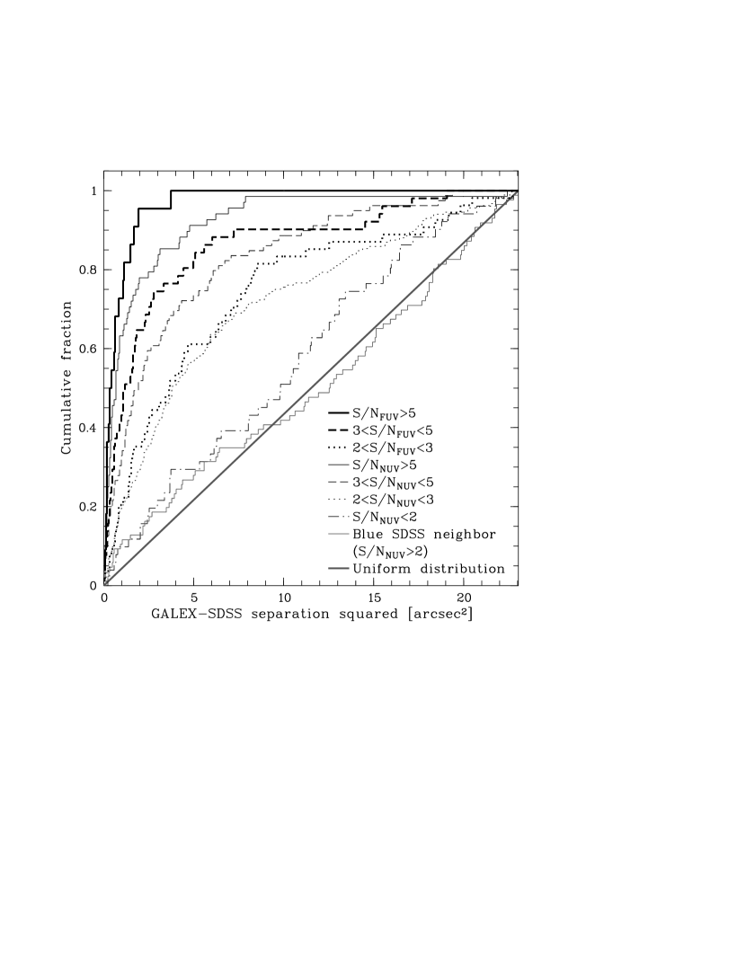
Figure 1.— Cumulative fraction of the squared separation between the GALEX positions and the optical position of GALEX-detected SDSS quasars. Thick (thin) black lines show FUV-optical (NUV-optical) distributions for various ranges in S/N. The thin gray line shows the cumulative distribution of the NUV-optical separations of SDSS quasars having blue optical neighbors within $\simeq$5″. The diagonal line denotes the uniform distribution with squared separation that is expected for false positives.

Figure 1 shows that for SDSS quasars without blue optical neighbors the distributions peak at small offsets with a clear dependence on S/N. Almost all FUV (NUV) S/N$>5$ detections are within $r\lesssim 2\arcsec$ ($r\lesssim 3\arcsec$) of the optical position with the difference being due to the better resolution in the FUV (Morrissey et al., 2007). At lower S/N the astrometric accuracy degrades and the rate of false positives should increase. At S/N${}_{\mathrm{NUV}}<2$ the cumulative fraction begins to resemble the one expected for false positives, with the excess indicating some real detections among them. Since the offset distributions at S/N${}_{\mathrm{NUV}}>2$ are much more concentrated, we infer that a limiting S/N$>2$ rather than a fixed limit in the matching radius yields a source catalog of high purity and completeness. Our chosen matching radius of $4.8\arcsec$ likely encompasses all true matches with S/N$>3$, whereas a few real $2<$S/N$<3$ detections (without neighbors) might exist at even larger separations. After excluding 117 ($\simeq 20$%) of the SDSS quasars with neighbors, restricting our catalog to S/N$>2$ (S/N$>3$) in at least one GALEX band reduces the number of potential (probable) detections to 601 (304).

We examined the GALEX source counts within 3′ around our quasars to estimate the probability of residual false matches between quasars and GALEX detections. Despite their low resolution, GALEX images are confusion-limited only in the longest DIS exposures (Hammer et al., 2010) due to the low source density in the UV. The measured density of S/N${}_{\mathrm{FUV}}>2$ detections in a typical MIS exposure is $\sim 1$/arcmin², which accounts for both real sources and false positives. At this low of a source density, the chance for any S/N${}_{\mathrm{FUV}}>2$ detection to fall in our 4.8″ aperture is small ($\lesssim 2\%$). Given that the source density on AIS plates is even lower, we conclude that essentially all FUV matches on AIS and MIS plates will correspond to optical sources within the chosen aperture. The rejection of SDSS quasars with blue neighbors probably excluded several real SDSS quasar matches (Fig. 1), so that we consider $\gtrsim 98\%$ of the remaining FUV-SDSS matches to be real. For non-SDSS quasars the remaining source confusion is more important than the rate of spurious detections. Adopting our SDSS neighbor fraction of $\sim 20\%$, we estimate a purity of $\sim 80\%$ for the quasars not imaged by SDSS. Due to the challenging reduction and analysis of DIS plates, we flagged the 23 quasars detected on DIS plates as still potentially affected by source confusion (only 7 are in the constrained sample discussed in §4.2).

2.4. Comparison to Source Matching in Syphers et al. (2009a)

Recently, Syphers et al. (2009a) published a catalog of 593 sources detected in GALEX GR4 and its small extension GR5. Apart from a slightly higher redshift cutoff ($z>2.78$) and a smaller matching radius (3″ around the quasar), their approach to source matching (not target selection) was similar to ours. However, they admitted that they did not verify the redshifts of the 165 sources with GALEX GR4+5 counterparts stemming from the Véron-Cetty & Véron (2006) catalog. Syphers et al. (2009a) presented follow-up HST/ACS UV prism spectroscopy of one of these, J1943$-$1502, with an estimated slitless spectroscopic redshift of 3.3 (Crampton et al., 1997). In order to establish whether this object can be used for He II IGM studies, we obtained an optical spectrum with the Kast spectrograph at the 3-m Shane Telescope at Lick Observatory. We confirm J1943$-$1502 as a naturally UV-bright low-redshift emission line galaxy rather than a quasar (Fig. 2). We caution that the Syphers et al. (2009a) list of Véron-Cetty & Véron (2006) sources contains 41 more such candidates the redshifts of which should be confirmed before embarking on follow-up UV spectroscopy with HST. In addition, 5 other sources from the Véron-Cetty & Véron (2006) catalog that are listed by Syphers et al. (2009a) as GALEX-detected $z_{\mathrm{em}}>2.7$ quasars are actually at lower redshifts according to our visual inspection of their spectra.

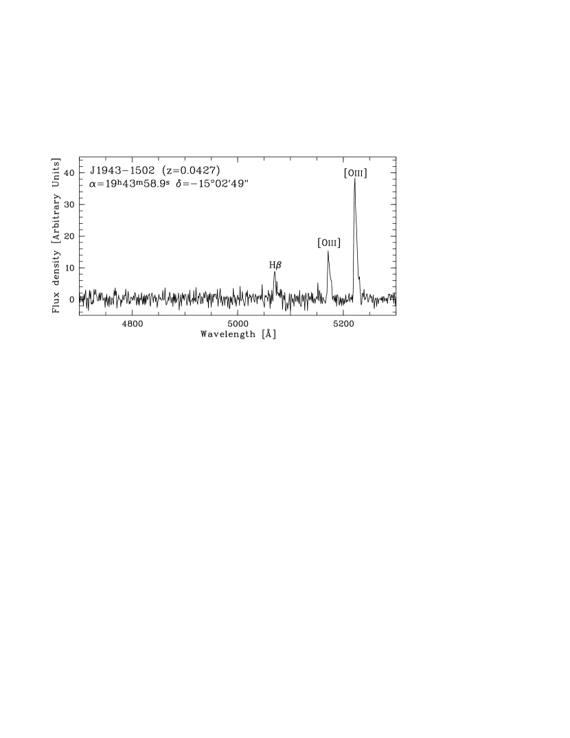
Figure 2.— Lick/Kast spectrum of the emission line galaxy J1943$-$1502 ($z=0.0427$). Identified emission lines are marked.

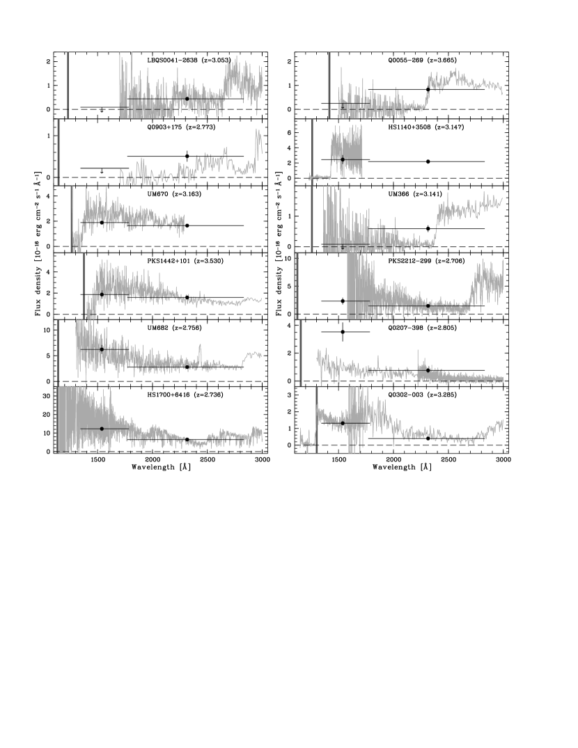
Figure 3.— HST spectra of 12 quasars (gray) and NUV & FUV fluxes measured by GALEX (filled circles with error bars and indicated bandpass). Arrows indicate upper limits from GALEX non-detections. Dashed lines mark zero flux. The thick vertical lines indicate the expected onset of He II absorption.

2.5. The GALEX UV colors of high-redshift quasars

The large sky coverage of GALEX enables the recovery of many UV-bright $z_{\mathrm{em}}>2.7$ quasars that have previously been followed up with HST to search for He II absorption by the IGM. GALEX recovers all 8 quasars known to show flux at He II Ly$\alpha$ that had been selected for observations before the launch of GALEX. Syphers et al. (2009a, b) recently confirmed 22 GALEX-selected sightlines to show He II, and all but the two listed only in GR1 are contained in the GALEX GR4 source catalog. 13 of the total 30 confirmed He II quasars are detected by GALEX at a low S/N$<3$, and we suspect that there is a larger population of UV-transparent quasars missed at the GALEX survey limit. We also recovered UV-bright quasars considered in previous photometric and spectroscopic surveys for He II with HST, the sightlines of which are intercepted by optically thick Lyman limit systems redward of the onset of He II absorption.

Table 1Data on the UV-bright quasars shown in Fig. 3

Object	$z_{\mathrm{em}}$	$m_{\mathrm{FUV}}$ [AB]	$m_{\mathrm{NUV}}$ [AB]	HST spectrum	$z_{\mathrm{LLS}}$	References
PKS 2212$-$299	$2.706$	$20.74$	$20.35$	STIS G230L	$0.6329$	Rao et al. (2006)
HS 1700$+$6416	$2.736$	$18.94$	$18.74$	FOS G130H/G190H/G270H	$\cdots$	Reimers et al. (1992); Evans & Koratkar (2004)
UM 682	$2.756$	$19.68$	$19.65$	FOS G160L/PRISM	$\cdots$	HST Archive
Q 0903$+$175	$2.773$	$>23.32$	$21.50$	FOS G160L/G270H	BAL	Turnshek et al. (1996)
Q 0207$-$398	$2.805$	$20.29$	$21.07$	FOS G160L/G270H	$\cdots$	Bechtold et al. (2002)
LBQS 0041$-$2638	$3.053$	$>24.32$	$21.67$	STIS G230L	$1.38:$	HST Archive
UM 366	$3.141$	$>24.40$	$21.35$	FOS G160L/G270H	$1.6128$	Rao & Turnshek (2000); Evans & Koratkar (2004)
HS 1140+3508	$3.147$	$20.68$	$19.92$	STIS G140L	$0.557$	HST Archive
UM 670	$3.163$	$20.97$	$20.22$	FOS G160L	$0.47:$	Lyons et al. (1994); Evans & Koratkar (2004)
Q 0302$-$003	$3.285$	$21.37$	$21.76$	STIS G140L/G230L	$\cdots$	Jakobsen et al. (1994); Heap et al. (2000)
PKS 1442$+$101	$3.530$	$20.98$	$20.26$	FOS G160L/PRISM	$0.621:$	Lyons et al. (1995); Evans & Koratkar (2004)
Q 0055$-$269	$3.665$	$>23.17$	$20.97$	FOS G160L/PRISM	$1.5335$	Cristiani et al. (1995); Evans & Koratkar (2004)

In Fig. 3 we compare the GALEX fluxes of 12 quasars to their UV spectra taken with HST. Their GALEX UV magnitudes are provided in Table 1 together with references to the UV spectra and the Lyman limit systems zeroing the spectral flux (if any). As these quasars are bright in the UV they are imaged with GALEX at high S/N, so that the GALEX fluxes are in very good agreement with the HST spectrophotometry. More interestingly, we find that several opaque sightlines are just detected in the NUV, but not in the FUV as expected (LBQS 0041$-$2603, Q 0055$-$269 and UM 366 in Fig. 3). In contrast, quasars that show flux down to the onset of He II absorption are detected in both bands with the flux rising towards shorter wavelengths as it recovers from partial Lyman limit systems (HS 1700$+$6416 and Q 0302$-$003). Thus, the GALEX UV color $m_{\mathrm{FUV}}-m_{\mathrm{NUV}}$ can be used to efficiently distinguish between opaque sightlines (red UV color) and transparent ones (blue UV color). The only quasars that remain insensitive to this obvious color selection criterion are those caught by an optically thick Lyman limit break just in the narrow range between the GALEX FUV band and the onset of He II absorption (HS 1140$+$3508, UM 670, PKS 1442$+$101, PKS 2212$-$299 in Fig. 3). We also identify two FUV-detected quasars, the HST spectra of which do not extend to He II Ly$\alpha$ in the rest frame of the quasar, located near the UV sensitivity cutoff of HST (UM 682 and Q 0207$-$398). These two sightlines are likely transparent, as there are no obvious strong Ly$\alpha$ absorbers that could cause a Lyman limit break in the $\sim 200$Å gap to the onset of He II absorption.

With the additional quasars targeted in recent surveys for He II sightlines (Syphers et al., 2009a, b) we can confirm the trend that most quasars with flux down to He II Ly$\alpha$ show blue GALEX colors, whereas most fruitlessly targeted quasars are characterized by red colors (see Fig. 12 below). Although more uncertain at low S/N, the colors still distinguish both quasar populations at S/N$\gtrsim 3$. Excluding sources with neighbors, $\sim 50$% of the SDSS quasars in our sample are detected at S/N$>3$ in the NUV band, but are lacking a significant FUV detection (S/N${}_{\mathrm{FUV}}<2$), indicating the ubiquitous strong Lyman continuum absorption. In particular, FUV dropouts detected in the NUV at high significance likely correspond to optically thick Lyman limit breaks.

In the following sections we will further explore how to further constrain our sample by the GALEX UV color to select the most promising quasar sightlines to detect He II absorption. This requires one to create mock quasar spectra with appropriate H I absorption, and to perform GALEX photometry on them to relate the GALEX UV color to the Lyman continuum absorption along the line of sight.

3. Monte Carlo simulations of high-redshift quasar spectra

3.1. Monte Carlo model for the H I Lyman series and Lyman continuum absorption

3.1.1 General procedure

For the problem at hand we followed standard practice to generate Monte Carlo (MC) H I Lyman forest and Lyman continuum absorption spectra from the observed statistical properties of the Ly$\alpha$ forest (e.g. Møller & Jakobsen, 1990; Madau, 1995; Bershady et al., 1999; Inoue & Iwata, 2008). The spectra were generated under the null hypothesis that the Ly$\alpha$ forest can be approximated as a random collection of absorption lines (Voigt profiles) with uncorrelated parameters (redshift $z$, column density $N_{\mathrm{H\,I}}$ and Doppler parameter $b$). From the line list representing the H I absorber population on a given line of sight from $z=0$ to an emission redshift $z_{\mathrm{em}}$ we created absorption spectra of the Lyman series (up to Ly30). Individual resolved Voigt profiles were computed on $\Delta\lambda=0.05$Å pixels using the approximation by Tepper-García (2006). Lyman continuum absorption was included using the H I ionization cross section by Verner et al. (1996).

In order to accurately predict the far-UV attenuation of high-redshift quasars by the IGM we desired a model that successfully reproduces the observed statistical properties of the Ly$\alpha$ forest at all redshifts, in particular concerning high-column density absorbers. Considering the recent observational advances in Ly$\alpha$ forest statistics, we deviated from previous simple MC descriptions of the Ly$\alpha$ forest and adjusted our input parameters as detailed in the following.

3.1.2 The absorber redshift distribution function

In our MC model the number of H I absorbers per line of sight in a given redshift range is a Poisson process (Zuo & Phinney, 1993). The observed mean differential line density per unit redshift is commonly parameterized as a power law $\mathrm{d}n/\mathrm{d}z|_{\mathrm{forest}}\propto(1+z)^{\gamma}$ that results in an effective optical depth $\tau_{\mathrm{eff,\alpha}}\propto(1+z)^{\gamma+1}$ for Ly$\alpha$ (and higher order series) absorption (Zuo, 1993). While there is some evidence that the redshift evolution depends on the column density even in the low-column density Ly$\alpha$ forest, the uncertainties are still large due to the non-unique process to deblend the forest into a series of Voigt profiles especially at $z\gtrsim 3$, incompleteness at the lowest column densities ($\log N_{\mathrm{H\,I}}\lesssim 12.5$), and the paucity of moderate-column density ($\log N_{\mathrm{H\,I}}\gtrsim 14.5$) systems (Kim et al., 1997, 2002). We therefore chose to parameterize $\mathrm{d}n/\mathrm{d}z$ for absorbers with $12<\log N_{\mathrm{H\,I}}<19$ as a single power law, the parameters of which were fixed by requiring each simulated spectrum to be consistent with a specified power law in $\tau_{\mathrm{eff,\alpha}}(z)$. Observations point to a break at $z\sim 1.5$, below which there is little evolution both in the line density (e.g. Weymann et al., 1998; Kim et al., 2002; Janknecht et al., 2006) and the mean absorption in the Ly$\alpha$ forest $D_{\mathrm{A}}=1-\mathrm{e}^{-\tau_{\mathrm{eff,\alpha}}}$ (Kirkman et al., 2007). Thus, we assumed a broken power law for $\tau_{\mathrm{eff,\alpha}}(z)$. Knowing that a power-law line distribution generally will not yield a power law for $D_{\mathrm{A}}(z)$ assumed by Kirkman et al. (2007), we converted their $D_{\mathrm{A}}$ to $\tau_{\mathrm{eff,\alpha}}$ and obtained a fit $\tau_{\mathrm{eff,\alpha}}(z)=0.017\left(1+z\right)^{1.20}$ for $z\lesssim 1.6$. At $2\lesssim z\lesssim 4$ $\tau_{\mathrm{eff,\alpha}}$ has been precisely measured in high-resolution spectra (Kim et al., 2007; Faucher-Giguère et al., 2008; Dall’Aglio et al., 2008), and the remaining disagreement at $z\gtrsim 4$ is likely due to continuum uncertainties, where very few pixels remain unabsorbed even in high resolution spectra. We adopted the fit $\tau_{\mathrm{eff,\alpha}}=0.0062\left(1+z\right)^{3.04}$ from Dall’Aglio et al. (2008), valid at $1.8<z<4.6$. Note that the break redshift cannot be determined as the intersection of the two power laws, since this would require one to extrapolate $\tau_{\mathrm{eff,\alpha}}(z)$ beyond the quoted validity ranges. Since the break is observationally not well constrained, given the large scatter of $\tau_{\mathrm{eff,\alpha}}$ measurements at $1.7<z<2$ and the paucity of data at $z\sim 1.5$ (Kirkman et al., 2007), we adopted a break redshift of $z=1.5$ for the broken power law in $\tau_{\mathrm{eff,\alpha}}(z)$.

For $\log N_{\mathrm{H\,I}}\geq 19$ absorbers we had to assume different redshift evolution laws, both because these systems are generally excluded in fits of $\tau_{\mathrm{eff,\alpha}}(z)$, and due to the fact that their number densities seem to evolve much slower with redshift. For damped Ly$\alpha$ systems (DLAs, $\log N_{\mathrm{H\,I}}\geq 20.3$) we adopted $\mathrm{d}n/\mathrm{d}z|_{\mathrm{DLA}}=0.044\left(1+z\right)^{1.27}$, determined by Rao et al. (2006) over the redshift range $0<z<5$. Figure 4 compares the observed number densities of DLAs compiled by Rao et al. (2006) to mock number densities obtained on 4000 MC sightlines assuming their fit for $\mathrm{d}n/\mathrm{d}z|_{\mathrm{DLA}}$. For Super Lyman Limit systems (SLLSs, $19\leq\log N_{\mathrm{H\,I}}<20.3$) there are significantly less constraints in the literature. A maximum-likelihood power-law fit to the SLLS survey by O’Meara et al. (2007) yields $\mathrm{d}n/\mathrm{d}z|_{\mathrm{SLLS}}=0.034\left(1+z\right)^{2.14}$ at $1.8<z<4.2$, but extrapolation to lower redshifts underestimates the lower limit $n_{\mathrm{SLLS}}\gtrsim 2n_{\mathrm{DLA}}$ at $z<1.65$ given by Rao et al. (2006). Rather than a break in the number density of SLLSs, this probably indicates that a much larger redshift range is needed to accurately describe the number density evolution of the rare SLLSs. By constraining the slope to $1.27<\gamma_{\mathrm{SLLS}}<2.14$ (i.e. between the evolution rate of DLAs and the SLLS fit at high $z$), and considering the estimated total number of $z<1.65$ SLLSs by Rao et al. (2006) we obtained a rough constraint on the low-redshift evolution of SLLSs (dotted lines in Fig. 4). After binning the high-$z$ measurements by O’Meara et al. (2007) we determined $\mathrm{d}n/\mathrm{d}z|_{\mathrm{SLLS}}\simeq 0.066\left(1+z\right)^{1.70}$ by eye (Fig. 4), noting that these numbers are quite uncertain as the $z<2$ SLLS population is not well constrained.

3.1.3 The Doppler parameter distribution function

Although the Doppler parameter distribution function $\mathrm{d}n/\mathrm{d}b$ is not required to calculate the attenuation of quasars by the IGM below the Lyman limit, our MC simulations reproduce the observed effective optical depth in the Ly$\alpha$ forest instead of a line density distribution. As the equivalent width of the lines on the flat part of the curve of growth ($13.5\lesssim\log N_{\mathrm{H\,I}}\lesssim 18.5$) depends both on the column density $N_{\mathrm{H\,I}}$ and the Doppler parameter $b$, the line density that is consistent with our adopted $\tau_{\mathrm{eff,\alpha}}(z)$ implicitly depends on the Doppler parameter distribution. For simplicity, we adopted the single parameter distribution function suggested by Hui & Rutledge (1999), $\mathrm{d}n/\mathrm{d}b\propto b^{-5}\exp\left(-b^{4}/b_{\sigma}^{4}\right)$, with $b_{\sigma}=24\,\mathrm{km}\,\mathrm{s}^{-1}$ (Kim et al., 2001) independent of redshift and column density, and restricted to the plausible range $10\,\mathrm{km}\,\mathrm{s}^{-1}\leq b<100\,\mathrm{km}\,\mathrm{s}^{-1}$.

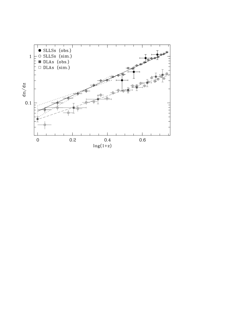
Figure 4.— Adopted differential number densities $\mathrm{d}n/\mathrm{d}z$ of SLLSs and DLAs as a function of redshift $z$. Filled symbols represent observed data (see text), whereas open symbols show the distributions recovered from 4000 MC simulations. The straight solid and dashed lines denote the power law fits to the observed data adopted for the simulations. The dotted lines show different normalizations to yield the number density of SLLSs at $z<1.65$ observed by Rao et al. (2006) adopting the slope of the DLA evolution law and the SLLS slope found at high $z$.

3.1.4 The column density distribution function

Previous studies on the IGM attenuation of high-redshift sources approximated the column density distribution function (CDDF) by a single or a broken power law, mainly driven by the reasonable approximation of the CDDF as a single power law $\mathrm{d}n/\mathrm{d}N_{\mathrm{H\,I}}\propto N_{\mathrm{H\,I}}^{-\beta}$ with $\beta\simeq 1.5$ over practically the full observable column density range (Tytler, 1987). However, more recent studies revealed significant deviations in the high-redshift CDDF from a single power law at intermediate ($14.5\lesssim\log N_{\mathrm{H\,I}}\lesssim 16$, Petitjean et al., 1993; Hu et al., 1995; Kim et al., 2002) and at the highest column densities ($\log N_{\mathrm{H\,I}}\gtrsim 19$, Storrie-Lombardi & Wolfe, 2000; Prochaska et al., 2005; O’Meara et al., 2007). A careful treatment of these systems is necessary, since even the intermediate column densities have a strong impact on the total LyC absorption (Madau, 1995; Haardt & Madau, 1996). However, due to the scarcity of $14.5\lesssim\log N_{\mathrm{H\,I}}\lesssim 17$ systems, the shape of the CDDF in this important range is presently not well constrained (Kim et al., 2002).

We took a novel approach to constrain the high-$z$ CDDF at $14.5<\log N_{\mathrm{H\,I}}<19$ by matching the mean free path (MFP) to Lyman limit photons calculated from the CDDF to our recent measurements from SDSS at $3.6<z<4.2$ (Prochaska et al., 2009, see also Prochaska et al. 2010). The effective optical depth to Lyman limit photons emitted at $z_{\mathrm{em}}$ and observed at $z_{\mathrm{obs}}$ is (e.g. Paresce et al., 1980)

$$\tau_{\mathrm{eff,LL}}\left(z_{\mathrm{obs}},z_{\mathrm{em}}\right) = \int_{z_{\mathrm{obs}}}^{z_{\mathrm{em}}}\int_{0}^{\infty}f\left(N_{\mathrm{H\,I}},z\right)$$ (1)

$$\times\left[1-\mathrm{e}^{-N_{\mathrm{H\,I}}\sigma_{\mathrm{LL}}\left(\frac{1+z}{1+z_{\mathrm{obs}}}\right)^{-3}}\right]\,\mathrm{d}N_{\mathrm{H\,I}}\mathrm{d}z,$$

with the Lyman limit photoionization cross section $\sigma_{\mathrm{LL}}=6.33\times 10^{-18}\mathrm{cm}^{2}$ and the frequency distribution of absorbers in redshift and column density $f\left(N_{\mathrm{H\,I}},z\right)=\frac{\partial^{2}n}{\partial N_{\mathrm{H\,I}}\partial z}$. Considering the different power-law redshift distributions of different absorber populations as outlined above, we approximated the CDDF as piecewise power laws that do not change over the considered redshift range, yielding

$$\tau_{\mathrm{eff,LL}}\left(z_{\mathrm{obs}},z_{\mathrm{em}}\right) = \sum_{j}C_{j}\int_{z_{\mathrm{obs}}}^{z_{\mathrm{em}}}\int_{N_{\mathrm{H\,I,min,j}}}^{N_{\mathrm{H\,I,max},j}}\left(1+z\right)^{\gamma_{j}}N_{\mathrm{H\,I}}^{-\beta_{j}}$$ (2)

$$\times\left[1-\mathrm{e}^{-N_{\mathrm{H\,I}}\sigma_{\mathrm{LL}}\left(\frac{1+z}{1+z_{\mathrm{obs}}}\right)^{-3}}\right]\,\mathrm{d}N_{\mathrm{H\,I}}\mathrm{d}z,$$

with different normalizations $C_{j}$ and power law exponents $\left(\gamma_{j},\beta_{j}\right)$ in different column density ranges $\left[N_{\mathrm{H\,I,min},j},N_{\mathrm{H\,I,max},j}\right]$. The normalization constants $C_{j}$ are the products of the line density normalizations $A_{j}$ ($\mathrm{d}n/\mathrm{d}z=A_{j}\left(1+z\right)^{\gamma_{j}}$) and the CDDF normalizations to yield an integral of unity in the respective column density range

$$C_{j}=\frac{A_{j}\left(1-\beta_{j}\right)}{N_{\mathrm{H\,I,max},j}^{1-\beta_{j}}-N_{\mathrm{H\,I,min},j}^{1-\beta_{j}}}.$$ (3)

For the SLLSs we assumed $\beta_{\mathrm{SLLS}}=1.4$ (O’Meara et al., 2007), whereas for DLAs we adopted $\beta_{\mathrm{DLA}}=2$ (Prochaska et al., 2005). We fixed the contributions of SLLSs and DLAs to $\tau_{\mathrm{eff,LL}}$ with our explicit line density evolutions. These absorbers are highly optically thick to LyC photons, so their incidence rather than their column density distribution determines their share to $\tau_{\mathrm{eff,LL}}$.

By definition the MFP corresponds to the proper distance where $\tau_{\mathrm{eff,LL}}=1$ for Lyman limit photons emitted at $z_{\mathrm{em}}$. In order to constrain the shape of the CDDF of Lyman limit systems and the Ly$\alpha$ forest, we considered a contiguous triple power law at $12<\log N_{\mathrm{H\,I}}<19$ that results in a quasi-continuous CDDF over the full column density range. Requiring the $12<\log N_{\mathrm{H\,I}}<19$ forest to result in our assumed power-law redshift evolution of the effective Ly$\alpha$ optical depth, we fixed $\gamma=2.04$ ($\gamma=0.20$) for $\log N_{\mathrm{H\,I}}<19$ at $z>1.5$ ($z\leq 1.5$). We then varied the triple power law CDDF, each time simulating 1000 MC sightlines at $0<z<4.6$ in order to determine the normalization constants for the line densities $A_{j}$ followed by computing the resulting total Lyman limit effective optical depth (eq. 2) and comparing the corresponding MFP at $3.6<z<4.2$ to our measurements (Prochaska et al., 2009).

In order to find the most plausible values for the slopes and breaks in the CDDF we considered additional observational constraints. The CDDF is best determined in the $z\sim 3$ Ly$\alpha$ forest and we adopted $\beta_{1}=1.5$ for $12<\log N_{\mathrm{H\,I}}<14.5$ at $z>1.5$ (e.g. Hu et al., 1995). At $\log N_{\mathrm{H\,I,max,1}}=14.5$ we imposed the first break in the CDDF to account for the deficit of absorbers at $\log N_{\mathrm{H\,I}}\gtrsim 14.5$ (e.g. Petitjean et al., 1993). Initially, we tried a single $\beta=1.5$ power law that strongly underpredicted the MFP, but remarkably extrapolates into the SLLS and DLA range where the CDDF was set independently. This probably reflects the fact that the $\beta=1.5$ power law approximation relies on both ends of the CDDF, which are by far the best constrained. We then varied the second break column density $N_{\mathrm{H\,I,max,2}}$ and the slope $\beta_{2}$ between the two breaks, requiring the slope $\beta_{3}$ at $\log N_{\mathrm{H\,I,max,2}}<\log N_{\mathrm{H\,I}}<19$ to meet the extrapolated $\beta=1.5$ power law at $\log N_{\mathrm{H\,I}}=19$, thus yielding a quasi-continuous CDDF, which we used at $z>1.5$.

Figure 5.— Comparison of the mean free path $\lambda_{\mathrm{mfp}}$ as a function of redshift $z$ resulting from our adopted redshift evolution and column density distribution of Ly$\alpha$ absorbers (open circles), direct measurements from Prochaska et al. (2009, filled circles) and the previous theoretical estimate by Madau et al. (1999). All values are reported for a flat cosmological model with $\left(\Omega_{\mathrm{m}},\Omega_{\Lambda}\right)=(0.3,0.7)$ and $H_{0}=72\,\mathrm{km}\,\mathrm{s}^{-1}\,\mathrm{Mpc}^{-1}$. The solid line shows a power law fit to our empirical estimates $\lambda_{\mathrm{mfp}}=50.14\left[\left(1+z\right)/4.6\right]^{-4.89}$ Mpc, valid for $z>3$. The dotted line shows the mean free path implied by a single $\beta=1.5$ power law at $\log N_{\mathrm{H\,I}}<19$ instead of the adopted broken power law.

Our calculations confirmed previous results that the MFP, and thus the mean LyC absorption at high redshift, is very sensitive to the shape of the CDDF at intermediate column densities (e.g. Madau, 1995). In particular, we could rule out many parameter combinations $\left(\log N_{\mathrm{H\,I,max,2}},\beta_{2}\right)$ by requiring the calculated MFP to be consistent with both the normalization and the redshift evolution of the measured MFP at $z>3.6$. In Fig. 5 we show our best match to the actual observations, obtained for $\left(\log N_{\mathrm{H\,I,max,2}},\beta_{2}\right)=(17.5,1.8)$, which imply a remarkably flat $\beta_{3}\simeq 0.9$. The modeled MFP agrees extremely well with the observed values and can be accurately described by a power law at $z>3$, yielding $\lambda_{\mathrm{mfp}}=50.14\left[\left(1+z\right)/4.6\right]^{-4.89}$ proper Mpc for a flat cosmology with $\left(\Omega_{\mathrm{m}},\Omega_{\Lambda}\right)=(0.3,0.7)$ and $H_{0}=72\,\mathrm{km}\,\mathrm{s}^{-1}\,\mathrm{Mpc}^{-1}$. In contrast, by adopting a featureless $\beta=1.5$ power law at $\log N_{\mathrm{H\,I}}<19$ together with the the slightly different distributions for the higher column density systems, the MFP is smaller by a factor $\simeq 2.3$ and is strongly inconsistent with the MFP measurements. The very good agreement between this underestimate and the MFP adopted by Madau et al. (1999) is not too surprising, as they assumed a single $\beta=1.5$ and a single absorber population evolving with redshift at $\gamma=2$, very similar to the $\gamma=2.04$ we adopted for $\log N_{\mathrm{H\,I}}<19$. We emphasize that at least two inflections in the CDDF are required at $\log N_{\mathrm{H\,I}}<19$ in order to yield a quasi-continuous CDDF that is consistent with our direct MFP measurements (see also Prochaska et al., 2010).

Figure 6 shows the corresponding model CDDFs at $z=4$ (covered by our MFP measurements) and $z=2$ (extrapolated from higher redshifts using the redshift evolution laws from Section 3.1.2). The CDDF at $\log N_{\mathrm{H\,I}}>19$ is remarkably smooth, given that independent and uncertain redshift evolution laws set the CDDF normalization there. The requirement for the CDDF to match the $\beta=1.5$ power law extrapolation from the low column density forest at $\log N_{\mathrm{H\,I}}\simeq 19$ yields a continuous CDDF, both at $z=4$ and at $z=2$, as intended.

As a consistency check we used our chosen distribution parameters to predict the incidence of Lyman limit systems (LLSs; $\log N_{\mathrm{H\,I}}\geq 17.2$). Figure 7 compares the mock differential number densities of LLSs to observations based on line counting (Stengler-Larrea et al., 1995; Péroux et al., 2003; Prochaska et al., 2010; Songaila & Cowie, 2010). Given the large statistical and systematic uncertainties in the observations, the agreement is remarkable, even at $1.5<z<3.6$, where we rely on the CDDF extrapolation from higher redshifts. While our MFP measurements tightly constrain the incidence of LLSs at $z>3.6$, the extrapolated CDDF might underestimate the incidence of LLSs if the CDDF straightens at lower $z$. By the same token, if LLSs evolve as strongly as indicated by Prochaska et al. (2010), we might have underestimated the MFP at $z<3.6$. Our prediction for the evolution of LLSs is most consistent with the fit by Stengler-Larrea et al. (1995), who sampled $z\sim 3$ based on earlier studies. Better models and predictions hinge on measurements of the MFP and the incidence of LLSs at $z\simeq 2$–3.

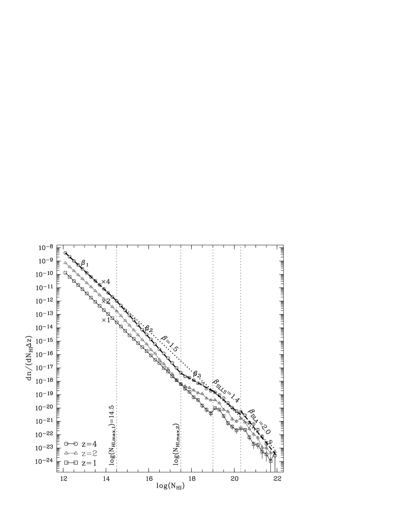
Figure 6.— Modeled column density distribution functions (CDDFs) $\mathrm{d}n/\left(\mathrm{d}N_{\mathrm{H\,I}}\Delta z\right)$ as a function of H I column density $N_{\mathrm{H\,I}}$ in a range $\Delta z=0.1$ around $z=1$, $z=2$ and $z=4$. For clarity the CDDFs have been scaled by the indicated factors. The symbols represent the binned CDDFs recovered from 4000 MC sightlines. The thick dashed lines show fits to the column density distribution at $z=4$ with the different slopes adopted in different column density regions (vertical dotted lines) designed to yield the measured MFP and its redshift evolution. The thick dotted line shows the CDDF at $z=4$ adopted for the forest ($\beta=1.5$) extrapolated to high column densities. Note that the redshift distributions and CDDFs in the SLLS and DLA range are set independently, whereas continuity is required for $\log N_{\mathrm{H\,I}}<19$.

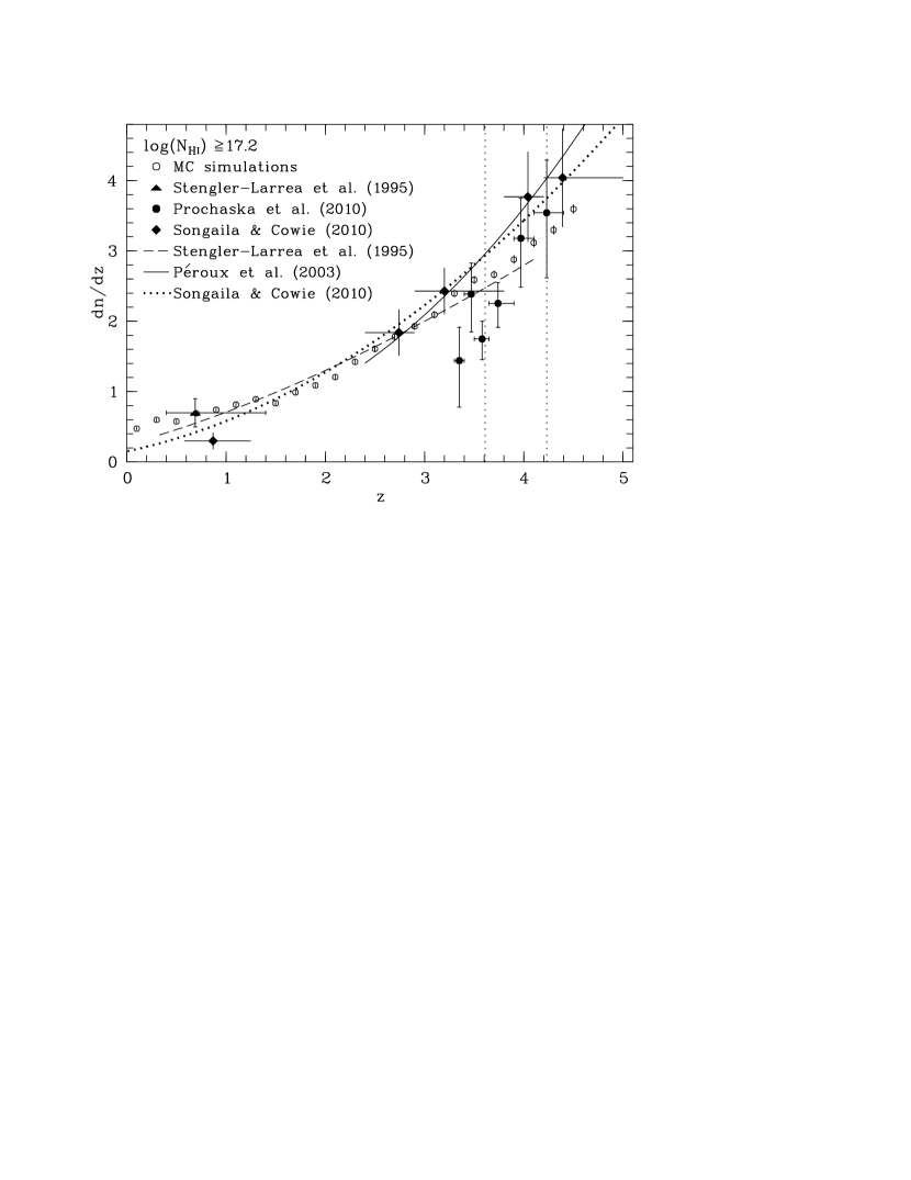
Figure 7.— Differential number density $\mathrm{d}n/\mathrm{d}z$ for Lyman limit systems ($\log{N_{\mathrm{H\,I}}}\geq 17.2$) as a function of redshift $z$ predicted from our MC simulations (open circles) compared to power law fits to actual data from Stengler-Larrea et al. (1995) (dashed), Péroux et al. (2003) (solid) and Songaila & Cowie (2010) (thick dotted) in their quoted validity range. The filled symbols show actual measurements (Stengler-Larrea et al., 1995; Prochaska et al., 2010; Songaila & Cowie, 2010). Note that the fit from Songaila & Cowie (2010) includes previous data from Stengler-Larrea et al. (1995) at low $z$ and Péroux et al. (2003) at high $z$. The vertical dotted lines mark the redshift range of our MFP measurements which constrain the number of Lyman limit systems in the MC simulations.

At low redshifts the CDDF is considerably less constrained, as the declining line density requires large samples of sightlines to be observed from space. Janknecht et al. (2006) determined a single power law for the CDDF at $0.5<z<1.9$ with $\beta=1.6$, but their fit is dominated by the low column density forest and slightly overpredicts the fraction of $\log N_{\mathrm{H\,I}}\gtrsim 14.5$ lines (their Fig. 5). Lehner et al. (2007) found that the $z<0.4$ CDDF steepens further at low column densities, whereas $\log N_{\mathrm{H\,I}}\gtrsim 14.5$ lines show a flatter slope $\beta\sim 1.5$. The low-redshift observations are inconsistent with our high-$z$ model CDDF with its inferred low abundance of $14.5\lesssim\log N_{\mathrm{H\,I}}\lesssim 17.5$ absorbers. For simplicity, we therefore assumed a featureless power law at $z<1.5$ for the column density range $12<\log N_{\mathrm{H\,I}}<19$, the slope of which was constrained by requiring a rough match to the CDDF at $\log N_{\mathrm{H\,I}}\approx 19$ (set independently by the SLLS distribution from above), while yielding the observed number of LLSs at low redshifts (Stengler-Larrea et al., 1995) and preserving the continuity in $\mathrm{d}n/\mathrm{d}z$ for LLSs predicted from our extrapolation from higher redshifts (Fig. 7). A slope $\beta=1.55$ matched these requirements. As an example, we show the modeled $z=1$ CDDF in Fig. 6. A lower incidence of LLSs at $z\sim 1$ as recently indicated by Songaila & Cowie (2010) would not drastically change our predictions, because the total LyC absorption at the He II edge primarily depends on the sparsely sampled redshift range $z\simeq 2$–3.

Table 2Monte Carlo simulation parameters

$z$ range	$z$ norm.	$\gamma$	$N_{\mathrm{H\,I}}$ range	$\beta$	$b_{\sigma}$	$b$ range
			[cm-2]		[km s-1]
$\left[0.0,1.5\right]$	$B=0.0170$	$0.20$	$\left[10^{12.0},10^{19.0}\right)$	$1.55$	$24$	$\left[10,100\right)$
$\left(1.5,4.6\right]$	$B=0.0062$	$2.04$	$\left[10^{12.0},10^{14.5}\right)$	$1.50$	$24$	$\left[10,100\right)$
$\left(1.5,4.6\right]$	$B=0.0062$	$2.04$	$\left[10^{14.5},10^{17.5}\right)$	$1.80$	$24$	$\left[10,100\right)$
$\left(1.5,4.6\right]$	$B=0.0062$	$2.04$	$\left[10^{17.5},10^{19.0}\right)$	$0.90$	$24$	$\left[10,100\right)$
$\left[0.0,4.6\right]$	$A=0.0660$	$1.70$	$\left[10^{19.0},10^{20.3}\right)$	$1.40$	$24$	$\left[10,100\right)$
$\left[0.0,4.6\right]$	$A=0.0440$	$1.27$	$\left[10^{20.3},10^{22.0}\right)$	$2.00$	$24$	$\left[10,100\right)$

With our final set of input parameters (Table 2) we computed 4000 MC line lists over the relevant redshift range $0\leq z\leq 4.6$. The number of sightlines is large enough to reach convergence in the incidence of optically thick H I absorbers even at low redshifts (Figs. 4 & 7), thus providing sufficient statistics for the highly stochastic UV LyC absorption.

3.2. Mock quasar photometry

We used another Monte Carlo routine to generate mock quasar catalogs, i.e. distributions in emission redshift and observed magnitude, from the observed luminosity function of quasars. Due to the strong attenuation by the IGM, only quasars that are intrinsically bright in the continuum redward of H I Ly$\alpha$ can be detected with current UV instruments. Thus, we adopted the SDSS DR3 luminosity function (Richards et al., 2006) that is well determined at bright magnitudes. We integrated their $z_{\mathrm{em}}>2.4$ pure luminosity evolution model of the differential luminosity function in the observed $i$ band at redshift two $\phi\left(M_{i}^{z_{\mathrm{em}}=2},z_{\mathrm{em}}\right)$ combined with the comoving volume in their adopted cosmological model to determine the all-sky surface counts of quasars in a given range of redshift and absolute magnitude

$$C_{4\pi}=\int_{z_{\mathrm{min}}}^{z_{\mathrm{max}}}\int_{M_{i,\mathrm{min}}^{z_{\mathrm{em}}=2}}^{M_{i,\mathrm{max}}^{z_{\mathrm{em}}=2}}\phi\left(M_{i}^{z_{\mathrm{em}}=2},z_{\mathrm{em}}\right)\frac{\mathrm{d}V(z_{\mathrm{em}})}{\mathrm{d}z_{\mathrm{em}}}\,\mathrm{d}M_{i}^{z_{\mathrm{em}}=2}\,\mathrm{d}z_{\mathrm{em}}.$$ (4)

We chose to convert from absolute magnitude $M_{i}^{z_{\mathrm{em}}=2}$ to $m_{1450}$, the observed AB magnitude at $1450$Å in the quasar rest frame, via the relation $M_{i}^{z_{\mathrm{em}}=2}=M_{1450}-1.486$ (Richards et al., 2006), yielding

$$m_{1450}=M_{i}^{z_{\mathrm{em}}=2}+5\log{\left(\frac{d_{L}}{\mathrm{Mpc}}\right)}-2.5\log{\left(1+z_{\mathrm{em}}\right)}+26.486$$ (5)

with the luminosity distance $d_{L}(z_{\mathrm{em}})$. By varying the integration limits of Equation 4 we obtained a parameterization for $\partial C_{4\pi}/\partial z_{\mathrm{em}}$ and $\partial C_{4\pi}/\partial m_{\mathrm{1450}}$ which we used to simulate $\sim 200000$ pairs $(z_{\mathrm{em}},m_{\mathrm{1450}})$ at $2.6<z_{\mathrm{em}}<4.6$ and $15<m_{\mathrm{1450}}<19$. This large mock sample ensured an accurate sampling of the rare UV-bright population of quasars transparent at the He II edge (see §4.1 below). For comparison, Equation 4 predicts just $\sim 11000$ quasars on the full sky over the same range in redshift and magnitude.

For each simulated quasar we assumed a unique spectral energy distribution modeled as a power law $f_{\nu}\propto\nu^{-\alpha}$ with a break at H I Ly$\alpha$ (Telfer et al., 2002), normalized to yield the modeled $m_{\mathrm{1450}}$. Redward of the break we assumed a Gaussian distribution of spectral slopes with $(\left<\alpha_{\mathrm{cont}}\right>,\sigma\left(\alpha_{\mathrm{cont}}\right))=(0.5,0.3)$ whereas blueward of the break we assumed $(\left<\alpha_{\mathrm{UV}}\right>,\sigma\left(\alpha_{\mathrm{UV}}\right))=(1.6,0.6)$ consistent with the large variation in far-UV spectral slopes found by Telfer et al. (2002). To the quasar continua we added the major quasar emission lines in the spectral range of interest (Ly$\beta$, Ly$\alpha$, N V, Si IV+O IV], C IV, C III], Mg II). The emission lines were modeled as Gaussian profiles, the strengths and widths of which were chosen consistent with Vanden Berk et al. (2001), with small variations from quasar to quasar.

Lastly we blanketed each spectrum blueward of H I Ly$\alpha$ by H I absorption in the IGM. For a given model quasar at a redshift $z_{\mathrm{em}}$ we randomly drew one of our 4000 MC sightlines and computed the H I Lyman series and continuum absorption at $0<z<z_{\mathrm{em}}$ (§ 3.1.1), yielding a final mock quasar spectrum at 912Å$<\lambda<$12000Å. Blueward of He II Ly$\alpha$ we assumed a He II Gunn-Peterson trough, resulting in zero flux (a reasonable assumption since the GALEX FUV band covers the He II break at $z_{\mathrm{em}}>3.44$). We then obtained mock SDSS $ugriz$ photometry (asinh magnitudes, Lupton et al., 1999) and mock GALEX FUV & NUV photometry (AB magnitudes) using the published filter curves (Morrissey et al., 2005). As Galactic extinction becomes important in the UV, we also computed the magnitudes after reddening each spectrum by the Galactic extinction curve (Cardelli et al., 1989), adopting $R_{V}=3.1$ and a lognormal distribution in $E(B-V)$ that closely resembles the color excess distribution towards SDSS quasars (Schneider et al., 2007). At the high Galactic latitudes considered here, the average extinction is $\simeq 0.26$ mag and $\simeq 0.22$ mag in the FUV and NUV, respectively.

4. Results

4.1. The expected number of UV-bright quasars at $z>2.7$

For each of our $\sim 200000$ model quasars we calculated the total H I Lyman continuum optical depth $\tau_{\mathrm{LyC}}$ at He II Ly$\alpha$ in the quasar rest frame, i.e. the accumulated H I attenuation by $\left[0.33\left(1+z_{\mathrm{em}}\right)-1\right]<z<z_{\mathrm{em}}$ absorbers. This quantity characterizes the transparency of a sightline to the onset of the He II absorption, irrespective of lower-redshift LLSs that might truncate the spectrum in the He II forest region. We also computed the AB magnitude of the quasar at He II Ly$\alpha$

$$m_{304}=m_{1450}+0.191\alpha_{\mathrm{cont}}+1.506\alpha_{\mathrm{UV}}+1.086\tau_{\mathrm{LyC}},$$ (6)

which depends on the input quasar magnitude $m_{1450}$, the spectral slopes of the continuum blueward ($\alpha_{\mathrm{UV}}$) and redward ($\alpha_{\mathrm{cont}}$) of H I Ly$\alpha$ and $\tau_{\mathrm{LyC}}$.

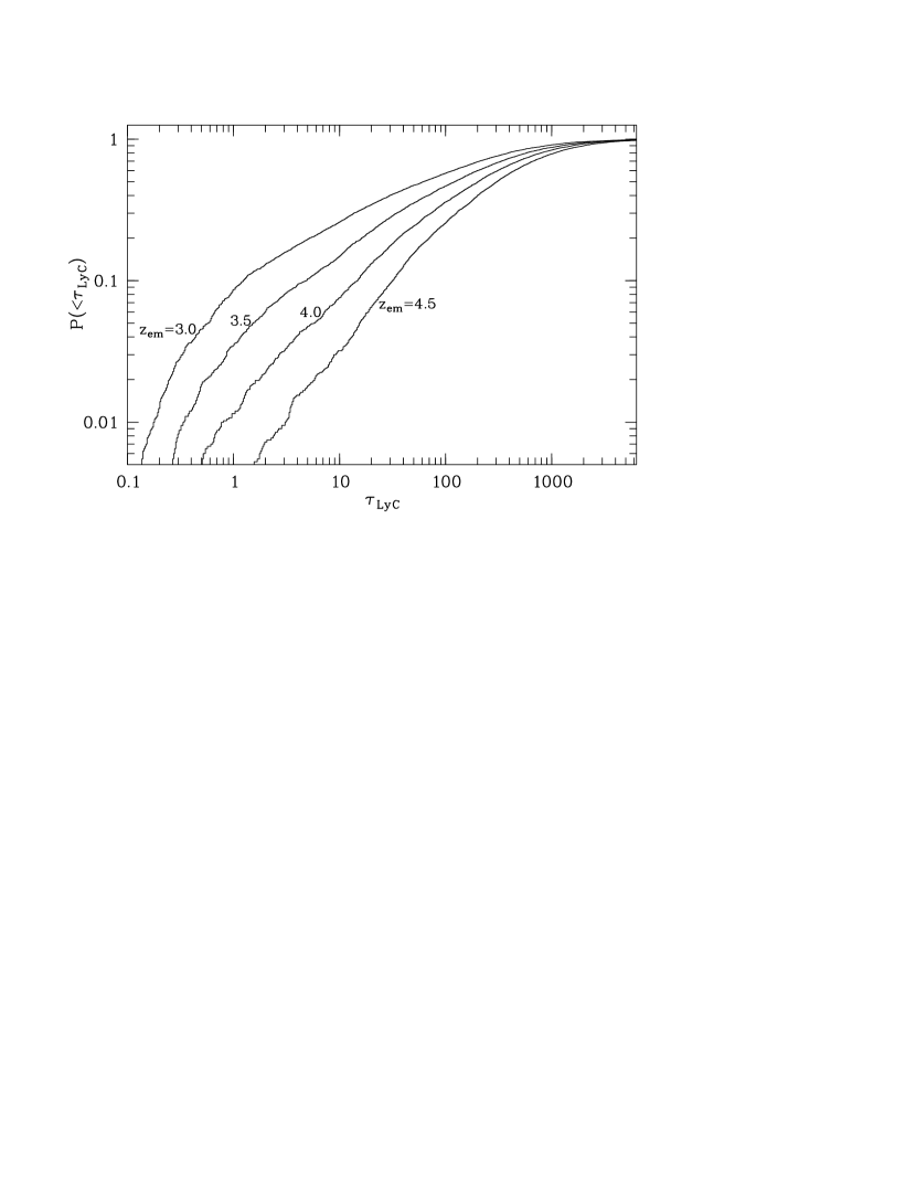
Figure 8.— Predicted cumulative probability distributions of the H I Lyman continuum optical depth $\tau_{\mathrm{LyC}}$ at He II Ly$\alpha$ in the rest frame of a source at redshift $z_{\mathrm{em}}$.

In Fig. 8 we plot the cumulative distribution function of $\tau_{\mathrm{LyC}}$ from our 4000 MC sightlines for different quasar emission redshifts. Our calculations indicate a very low probability to encounter a sightline that is not highly attenuated at the He II edge, consistent with previous estimates (Picard & Jakobsen, 1993; Jakobsen, 1998). The accumulated continuum optical depth strongly increases with emission redshift. While $\simeq 9$% of all quasars at $z_{\mathrm{em}}=3$ should be ’transparent’ ($\tau_{\mathrm{LyC}}<1$), this fraction drops to $\sim 1$% at $z_{\mathrm{em}}=4$.

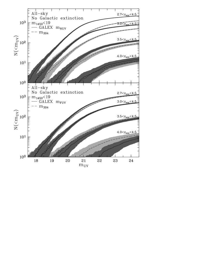
Figure 9.— Predicted cumulative all-sky number counts of $m_{1450}<19$ quasars as a function of limiting UV magnitude for various redshift ranges. The upper (lower) panel compares the predicted source counts in the GALEX NUV (GALEX FUV) band (solid lines) to the ones inferred at He II Ly$\alpha$ in the source rest frame (shown dashed in both panels), respectively. The gray shaded regions indicate $1\sigma$ errors in the source counts due to cosmic variance. Note that these predictions include the attenuation by the IGM, but they have not been corrected for Galactic extinction.

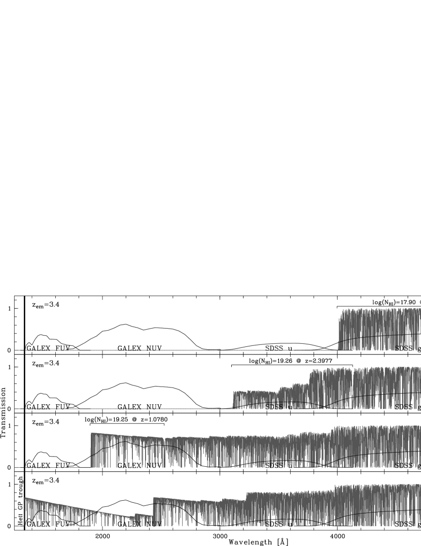
Figure 10.— Four simulated normalized H I forest Lyman series and Lyman continuum absorption spectra of a source at $z_{\mathrm{em}}=3.4$ with overplotted filter bandpasses. The upper three panels show sightlines with optically thick systems that result in photometric dropouts without recovery at the He II Ly$\alpha$ edge (vertical line). In the sightline shown in the uppermost panel, an intervening SLLS prevents the spectrum from recovering from the first encountered LLS break. The sightline in the lowest panel does not have an intervening optically thick absorber, so that the background source is detectable in all photometric bands until the onset of the assumed He II Gunn-Peterson trough.

The predicted number of high-$z$ quasars detectable in the far UV primarily depends on the increasing opacity and the declining quasar space density at $z_{\mathrm{em}}\gtrsim 3$. Figure 9 shows the predicted cumulative all-sky number counts of $m_{1450}<19$ quasars in the GALEX FUV & NUV bands compared to their predicted $m_{304}$ for various redshift ranges. These estimates have not been corrected for Galactic extinction, in particular close to the Galactic plane. For an $E(B-V)>1$ commonly encountered at Galactic latitudes $|b|\lesssim 20\arcdeg$, the FUV extinction is $>8$ mag, so that $\sim 25$% of the sky are effectively blocked for He II studies even if quasars are found in this ’Zone of Avoidance’ (Hubble, 1934).

The SDSS luminosity function predicts $\sim 9200$ $m_{1450}<19$ quasars on the entire sky at $2.7<z_{\mathrm{em}}<4.5$ (eq. 4). More than 200 of these should have $m_{304}<21$, well within the capabilities of HST. However, at $4<z_{\mathrm{em}}<4.5$ there should be just $\sim 600$ $m_{1450}<19$ quasars on the whole sky, the sightlines of which encounter larger LyC attenuation, yielding just $\sim 1$ quasar at $m_{304}<21$. At these high redshifts cosmic variance has a strong impact on the real number counts. The same is true for the least-attenuated UV-brightest quasars that are located at the lowest redshifts. In order to obtain accurate results both at the highest redshifts and the brightest UV magnitudes we had to simulate the large set of $\sim 200000$ quasars, corresponding to $\sim 20\times$ the predicted all-sky number counts.

The GALEX bands trace the small UV-transparent quasar population very well, but differently at different redshifts. At $z_{\mathrm{em}}<3.5$ the GALEX NUV band is not a good indicator for the flux at He II Ly$\alpha$ because of the high probability to encounter a Lyman limit break in the large wavelength range between the NUV band and the onset of He II absorption. As the FUV band is closer to the He II edge it is a more sensitive indicator of flux at He II Ly$\alpha$. At $z_{\mathrm{em}}>3.44$ the FUV band samples the He II edge and the presumed He II Gunn-Peterson trough. The He II Ly$\alpha$ absorption progressively attenuates the FUV flux and likely causes FUV dropouts at $z_{\mathrm{em}}>4$. Only at $z_{\mathrm{em}}>4$ will the GALEX NUV flux indicate a likely transparent sightline.

Figure 10 further illustrates the importance of detected FUV flux to select promising sightlines for He II absorption. We show the normalized H I Lyman series and Lyman continuum transmission spectra of four representative mock sightlines from the onset of the He II Gunn-Peterson trough to H I Ly$\alpha$ at the emission redshift $z_{\mathrm{em}}=3.4$. In the sightlines shown in the upper three panels the indicated optically thick H I absorbers truncate the spectra at the Lyman limit, causing dropouts in the overplotted filter bands. Obviously, only $z_{\mathrm{em}}\sim 3.4$ quasars detected in the GALEX FUV band will show a transparent sightline that has recovered from intervening LLS breaks. Even for the small subset of high-$z$ quasars detected by GALEX, intervening low-redshift LLSs likely truncate the quasar flux between the two GALEX bands. Thus, in order to select transparent sightlines at a high success rate, FUV detections are required at least at $z_{\mathrm{em}}<3.4$ where the FUV band still samples the quasar continuum redward of He II Ly$\alpha$.

4.2. Far-UV color selection of probable He II sightlines

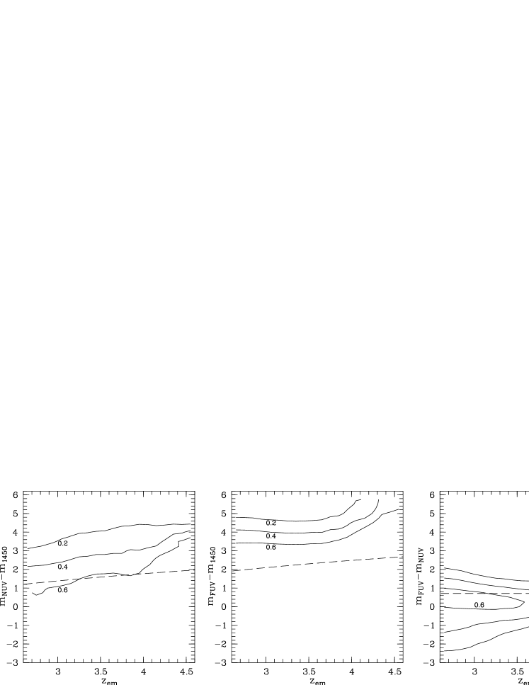
Figure 11.— Predicted colors of quasars detectable with GALEX as a function of emission redshift $z_{\mathrm{em}}$ (left: $m_{\mathrm{NUV}}-m_{\mathrm{1450}}$; middle: $m_{\mathrm{FUV}}-m_{\mathrm{1450}}$; right: $m_{\mathrm{FUV}}-m_{\mathrm{NUV}}$). The contours delineate the probability that a quasar at a given redshift $z_{\mathrm{em}}$ detected by GALEX at a given color will be transparent at the He II 304Å edge ($\tau_{\mathrm{LyC}}<1$). The dashed lines mark the colors of the mean adopted quasar spectral energy distribution (§3.2) ignoring intergalactic absorption.

Figure 10 also illustrates that the GALEX UV color $m_{\mathrm{FUV}}-m_{\mathrm{NUV}}$ can be used to select the most promising sightlines to discover He II absorption. Significantly red GALEX colors indicate low-$z$ LLS breaks (3rd panel of Fig. 10) between the FUV and the NUV band, whereas blue GALEX colors signal the recovery from a LLS break or the relatively unabsorbed hard quasar continuum. NUV-only detections indicate transparent sightlines only if the FUV band significantly covers the strong He II absorption, i.e. at very high redshift ($z_{\mathrm{em}}\gtrsim 4$).

We used our mock quasar photometry to determine the fraction of transparent sightlines (defined as the fraction of sightlines with $\tau_{\mathrm{LyC}}<1$) as a function of redshift. In Figure 11 we plot the probability contours that a quasar detected by GALEX at a given color will show a total $\tau_{\mathrm{LyC}}<1$ along the line of sight at He II Ly$\alpha$ in the quasar rest frame. The UV-optical colors $m_{\mathrm{NUV}}-m_{1450}$ and $m_{\mathrm{FUV}}-m_{1450}$ just give modest hints whether the quasar will show flux at He II Ly$\alpha$. The NUV-optical color indicates a transparent sightline just at the highest redshifts, but is otherwise quite insensitive due to the frequent low-$z$ LLS breaks between the NUV band and the He II edge. Thus, at any redshift the least-absorbed quasars with the bluest $m_{\mathrm{NUV}}-m_{1450}$ colors are the most promising candidates to detect He II. The FUV-optical color $m_{\mathrm{FUV}}-m_{1450}$ provides better constraints. Quasars at $z_{\mathrm{em}}<3.4$ at a $m_{\mathrm{FUV}}-m_{1450}\lesssim 3.4$ have a $\gtrsim 60$% chance to show a low $\tau_{\mathrm{LyC}}<1$ along the line of sight. At higher redshifts, the He II Gunn-Peterson trough reddens the FUV-optical color.

The UV color $m_{\mathrm{FUV}}-m_{\mathrm{NUV}}$ (right panel of Fig. 11) yields the most natural color-selection constraints. Any quasar detected in both GALEX bands at a rather blue UV color has a high chance to show flux at He II Ly$\alpha$. Unless the FUV fluxes get severely absorbed by He II at $z_{\mathrm{em}}\gtrsim 4$, the GALEX UV colors of transparent quasars should be similar to those of their unabsorbed spectral energy distributions, with the slightly bluer colors indicating the recovery from partial LLSs that result in a steeply rising flux towards the FUV due to the strong frequency dependence of the LyC cross-section. Quasars at $m_{\mathrm{FUV}}-m_{\mathrm{NUV}}\gtrsim 2$ are likely to show a LLS break at the blue end of the FUV band even if they are detected in the FUV. Very blue quasars below the lower 20% line in the right panel of Fig. 11 are recovering from a $\tau_{\mathrm{LL}}>1$ LLS break at $z>2$ so that their flux rises steeply in both GALEX bands.

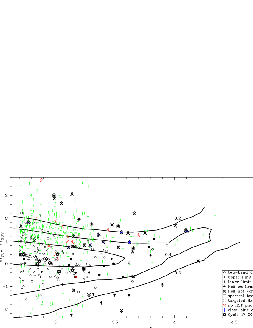
Figure 12.— GALEX UV color $m_{\mathrm{FUV}}-m_{\mathrm{NUV}}$ of $z_{\mathrm{em}}>2.7$ quasars in the GALEX GR4 source catalog. For quasars in the SDSS footprint without UV follow-up observations we only show those that do not have sufficiently blue neighboring objects out to 5″ separation to avoid GALEX source confusion. Open circles show quasars detected in both GALEX bands, whereas arrows indicate upper (lower) color limits for sources detected in the NUV (FUV) only. Filled circles indicate the UV colors of quasar sightlines spectroscopically confirmed to be transparent at He II Ly$\alpha$. Quasars showing low spectroscopic FUV flux, either due to a Lyman limit break in the FUV or a recovery from a Lyman limit break in the NUV, are shown as open squares. Thick crosses mark quasars targeted with HST, but not confirmed to show flux at He II Ly$\alpha$, either because of optically thick Lyman limit breaks in the FUV spectral range (crossed squares) or no detectable FUV flux at all (thick $\times$ crosses). Quasars without significant FUV flux in follow-up HST images are indicated as well (thin $\times$ crosses). Some spectroscopically observed quasars exhibit BAL features (diamonds), and several previous follow-up observations seem to have been affected by GALEX source confusion ($+$ signs). Thick star symbols mark the 8 UV-bright quasars we selected for upcoming follow-up spectroscopy with HST/COS in Cycle 17. The thick lines show the probability contours that a quasar at a given UV color shows flux down to the onset of the He II absorption, based on our MC simulations.

With these estimates on the UV color range of quasars that show flux at He II Ly$\alpha$, we can estimate He II detection probabilities for the actual GALEX-detected $z_{\mathrm{em}}>2.7$ quasars. Figure 12 compares the GALEX $m_{\mathrm{FUV}}-m_{\mathrm{NUV}}$ colors of our transparent ($\tau_{\mathrm{LyC}}<1$) mock quasars to actual observations. We find that the UV colors of quasars having sightlines that are known to be transparent down to the onset of He II absorption are similar to the simulated UV colors of transparent quasars. A posteriori, the blue UV colors of most known He II quasars indicate a high probability for transparency. Among the GALEX-detected quasars without further follow-up the rare quasars at $m_{\mathrm{FUV}}-m_{\mathrm{NUV}}\lesssim 1$ are the best candidates to search for flux at He II Ly$\alpha$. Our MC simulations indicate a probability of $\gtrsim 60$% that a $z_{\mathrm{em}}\lesssim 3.5$ quasar detected at $0\lesssim m_{\mathrm{FUV}}-m_{\mathrm{NUV}}\lesssim 1$ will show $\tau_{\mathrm{LyC}}<1$. The slight offset between the simulated and the observed UV colors of transparent quasars could be due to a generally harder UV spectral energy distribution than assumed in the simulations (i.e. $\left<\alpha_{\mathrm{UV}}\right><1.6$) and/or a higher mean LyC absorption from a larger population of $z\lesssim 2$ LLSs. We suspect the latter is more likely given the poor existing constraints on the exact CDDF and the evolution of the MFP at $z<3.6$ (§3.1.4).

In contrast, quasars confirmed by HST follow-up to show zero flux at He II Ly$\alpha$ are mostly redder in $m_{\mathrm{FUV}}-m_{\mathrm{NUV}}$ than the UV-transparent population, consistent with our simulations. Especially the high upper limits $m_{\mathrm{FUV}}-m_{\mathrm{NUV}}\gtrsim 2$ correspond to significant detections in the NUV, but no formal detection in the FUV, signaling the cutoff by an optically thick LLS. The only opaque sightlines that remain insensitive to our UV color selection are the ones intercepted by a LLS just within the narrow range between the blue end of the FUV bandpass and He II Ly$\alpha$ (e.g. PKS 1442$+$101 in Fig. 3). This is reflected in our simulations by the broadening color contours towards lower redshifts.

If the LLS is not optically thick then the flux can recover, but the quasar is of very limited scientific value because it is too faint for follow-up at He II Ly$\alpha$ (i.e. $\tau_{\mathrm{LyC}}>1$; Syphers et al. 2009a, b have identified two such quasars). Moreover, the two BALQSOs confirmed in the FUV by Syphers et al. show red GALEX UV colors, presumably due to their intrinsically redder spectral energy distributions and/or BAL troughs extending in the UV. While these quasars are interesting to study the BAL phenomenon, they are effectively useless for investigating intergalactic He II absorption as one cannot distinguish IGM He II Gunn-Peterson troughs from potential BAL troughs.

The UV color separates well between blue He II-transparent quasars and red opaque ones, despite the low S/N near the GALEX detection limit. However, quasars just detected in one of the GALEX bands require further attention. FUV-only detected sightlines probably recover from a partial LLS break so that the low NUV flux is beyond the detection limit. Given that we just quote $1\sigma$ flux limits on NUV dropouts, the colors of the 6 very blue confirmed He II quasars could be similar to those of the other He II quasars. Likewise, the FUV flux of some transparent quasars detected just in the NUV should have been detected as well. Nevertheless, since significant NUV-only detections indicate opaque sightlines, such background quasars should not be regarded as prime candidates for spectroscopic follow-up. Generally, we do not consider very low S/N$<2$ detections in a single GALEX band to be real, whereas sources detected in both GALEX bands probably are, as the GALEX pipeline performs the source detection independently before merging the catalogs (Morrissey et al., 2007).

Moreover, quasars with nearby optical neighbors should be avoided, as they will be likely affected by GALEX source confusion due to the broad instrument PSF. Apart from GALEX-detected $z_{\mathrm{em}}>2.7$ quasars with HST follow-up, Fig. 12 shows only those sources which qualify for further investigation (non-BAL, no blue neighboring source in SDSS DR7 at separation $<5\arcsec$). Given that the UV color is not well constrained at low S/N (a S/N$>3$ in both bands corresponds to $\sigma(m_{\mathrm{FUV}}-m_{\mathrm{NUV}})<0.51$) we consider two subsets of these quasars as the most promising ones for further detections of He II: (i) those 52 which have been significantly detected in both bands at S/N$>3$ and have $m_{\mathrm{FUV}}-m_{\mathrm{NUV}}<1$, and (ii) the 114 remaining quasars detected at S/N$>2$ in the FUV band. These samples are presented in Tables 3 and 4, respectively. We caution that several GALEX detections outside the SDSS DR7 footprint will correspond to confused GALEX sources ($\sim 20\%$ if we adopt our estimate from SDSS). Likewise, a few quasars with red optical neighbors (flagged in Tables 3 and 4) might be confused sources, since our neighbor classification was based on the broadband SED shape from SDSS and GALEX. Seven quasars detected on DIS survey plates have been flagged as potentially affected by source confusion. The majority (90%) of the $z_{\mathrm{em}}>2.78$ quasars in Tables 3 and 4 were previously suggested as candidate He II quasars by Syphers et al. (2009a). All but one of the 13 additional $z_{\mathrm{em}}>2.78$ quasars have GALEX counterparts beyond the match radius adopted by Syphers et al. 2009a (3″).

5. Application to the Sloan Digital Sky Survey

5.1. Comparing UV-bright SDSS quasars to predictions

With a homogeneous well-characterized large area quasar survey such as SDSS, we can compare our predicted number counts of UV-bright quasars to actual observations after accounting for several observational effects. First, the predicted all-sky number counts (Fig. 9) were corrected for Galactic foreground extinction as incorporated in our calculations (§3.2). Then we accounted for the actual GALEX GR4 sky coverage and depth. The exposure time varies significantly among tiles of a given GALEX imaging survey, rendering them inherently inhomogeneous. Therefore we used the GALEX instrument sensitivity (Morrissey et al., 2007) and the actual GR4 tile exposure times to calculate a $5\sigma$ limiting magnitude for each tile. With an approximate area correction for the overlapping circular GALEX tiles (e.g. Budavári et al., 2009) we then calculated the GR4 sky coverage as a function of limiting magnitude. We regard the S/N$\geq 5$ threshold as sufficient to avoid incompleteness in the GALEX source catalog, but we note that apart from general source counts (Bianchi et al., 2007) the repeatability and S/N stability of GALEX is not well established at its instrumental limit.

Next, we accounted for the SDSS sky coverage. Considering that GALEX GR4 covers almost the full sky at high Galactic latitude ($|b|\gtrsim 20\arcdeg$), we avoided the cumbersome calculation of the actual overlapping area of SDSS DR7 and GALEX GR4 (see Budavári et al. 2009 for an application to DR6+GR3), and adopted instead the SDSS Legacy spectroscopic sky coverage of 8032 deg². SEGUE fields were not taken into account, as they are mainly at low Galactic latitude and have a significantly smaller quasar targeting rate. Lastly, we corrected for the SDSS quasar selection efficiency to predict the number of UV-bright SDSS quasars detectable with GALEX. As SDSS selects quasars primarily by color, we used the photometric SDSS selection function by Richards et al. (2006) averaged at $i<19.1$. The magnitude cut provides a homogeneous survey limit at $z_{\mathrm{em}}>2.7$ (SDSS selects $z\gtrsim 3$ quasar candidates at $i<20.2$) and ensures that the selection function does not depend on magnitude. Moreover, it is well matched to the rest-frame magnitude limit we applied in our simulations ($i\sim m_{1450}<19$), as the $i$ band covers the quasar continuum redward of Ly$\alpha$ at the relevant redshifts. The different bandpasses induce a slight redshift-dependent offset $i-m_{1450}\sim-0.1$, but uncertainties in the $K$ correction used to determine the quasar luminosity function are larger than this.

From our sample of quasars we then selected only those 58 which were targeted by SDSS, have $i<19.0$ and have been detected by GALEX at S/N$>5$ in the NUV band. If we exclude SDSS quasars with blue optical neighbors that could be cases of GALEX source confusion, this number reduces to 52. Figure 13 compares the cumulative number counts of these NUV-detected quasars to the prediction based on our IGM model and the SDSS selection function by Richards et al. (2006, upper curve). Adopting the Richards et al. (2006) selection efficiency, the number of NUV-detectable quasars is a factor of $\sim 2$ larger than observed, even including potentially confused GALEX sources. The predicted number counts can only be lowered by increasing the LyC opacity in our IGM model or by decreasing the SDSS selection efficiency. The uncertainties on other model ingredients, such as the luminosity function of bright quasars, the $K$ correction, and the GALEX+SDSS footprint corrections, are too small to create this discrepancy. Given that our IGM model fits the MFP measurements (Fig. 5) and independently reproduces the observed redshift evolution of LLSs (Fig. 7) we have focused here on systematic effects in the SDSS selection efficiency.

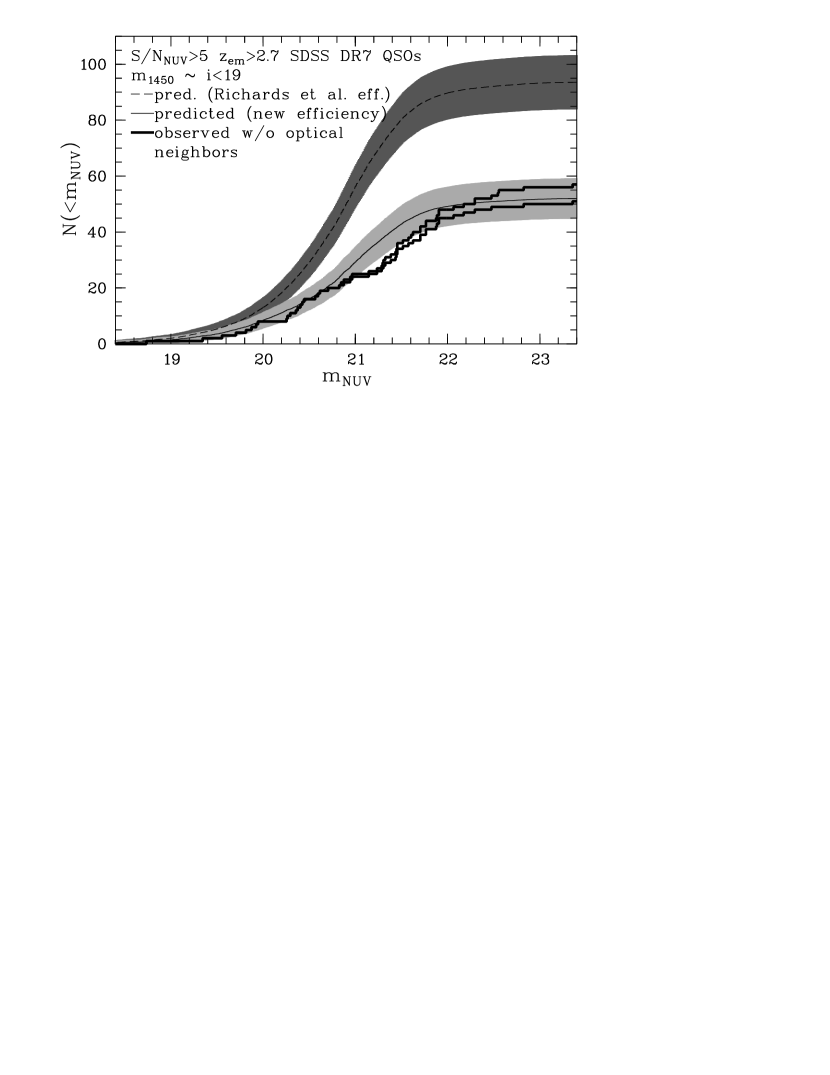
Figure 13.— Comparison of predicted and observed cumulative number counts of $z_{\mathrm{em}}>2.7$ $i\lesssim 19$ SDSS DR7 quasars detectable with GALEX at S/N$>5$ in the NUV. The thin lines plot the predicted number counts using the SDSS color selection efficiency from Richards et al. (2006, dashed), and our color-dependent selection efficiency (solid), respectively. Shaded regions outline Poisson errors on the source counts. The thick solid lines show the observed cumulative number counts of SDSS DR7 w/o potentially confused GALEX detections due to nearby blue optical neighbors.

5.2. A color-dependent SDSS color selection function

Quasar selection by broadband colors is expected to be inefficient and highly model-dependent at $z\sim 3$, where quasar colors are similar to those of main-sequence stars (e.g Richards et al., 2006). We used the simulated SDSS photometry of our $\sim 200000$ $z_{\mathrm{em}}>2.6$ model quasars (§3.2) to reassess the SDSS quasar selection function. SDSS selects most quasar candidates as outliers from the stellar locus in multi-dimensional color space. Because this procedure depends on the photometric errors, we computed these by fitting the photometric errors of observed $z_{\mathrm{em}}>2.7$ SDSS DR5 quasars (Schneider et al., 2007) as a function of magnitude. We associated each mock SDSS magnitude $m$ with the fitted mean photometric error $\sigma_{m}$ without modifying the mock magnitude. Thus, we assume perfect SDSS photometry with a realistic mean error, which simplifies our further discussion, but will likely result in an overestimate of the selection efficiency due to photometric uncertainties near the SDSS survey limit, particularly in the $u$ band. Potential effects of asymmetric distribution functions of SDSS magnitudes and their errors at the survey limit are beyond the scope of this paper.

Gordon Richards kindly agreed to process our mock photometry with the final SDSS quasar target selection algorithm (Richards et al., 2002) that incorporates the imposed 10% follow-up targeting rate of quasars whose colors intersect the stellar locus (the ’mid-$z$’ inclusion box of Richards et al. 2002). The result of that operation is a selection flag for each mock quasar indicating whether it would have been targeted under SDSS routine operations. We then computed average SDSS selection efficiency as the fraction of selected mock quasars in $\Delta z_{\mathrm{em}}=0.05$ bins.

In Fig. 14 we compare our selection function to the one by Richards et al. (2006). Both selection functions are essentially unity at $z_{\mathrm{em}}\gtrsim 3.6$ where colors of quasars are sufficiently red because of IGM absorption to separate well from the stellar locus. In particular, high-redshift LLSs will result in red $u-g$ colors due to $u$ band dropouts (Fig. 10). At $z_{\mathrm{em}}\lesssim 3.5$, however, there is a striking difference between the two selection functions. Our average selection efficiency at $z_{\mathrm{em}}\simeq 3.2$ is $\sim 25$% smaller than the one by Richards et al. (2006), whereas at $z_{\mathrm{em}}\simeq 2.7$ it is a factor of $\sim 4$ higher, and is in better agreement with their upper limit based on the expected smoothness of the luminosity function with redshift. The main model ingredients affecting the colors, and thus the selection efficiency, are the quasar spectral energy distributions and the IGM, i.e. the LyC absorption. Apart from a larger spread in the power-law spectral index blueward of H I Ly$\alpha$, our parameters to model the intrinsic quasar spectra are very similar to the ones used by Richards et al. (2006), so these discrepancies must be due to different assumptions regarding the properties of the IGM that result in statistically different quasar colors.

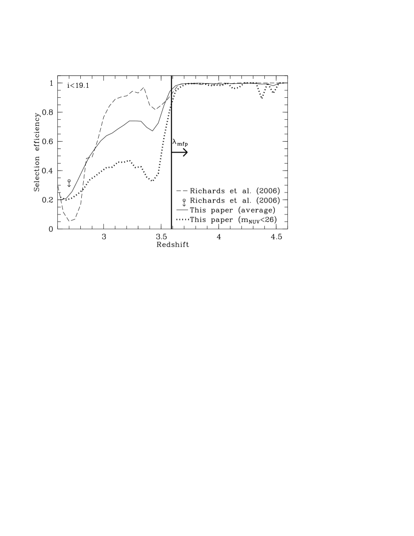
Figure 14.— Average SDSS quasar color selection efficiency derived using our MC simulations of SDSS photometry (solid line) compared to the previous estimate by Richards et al. (dashed line). The average selection efficiency is almost magnitude-independent for the bright $i<19.1$ quasars considered here. The open circle marks the lower limit on the $z\simeq 2.7$ selection efficiency estimated by Richards et al. (2006) by requiring a smooth luminosity function at lower and higher redshifts. The thick dotted line shows the SDSS color selection efficiency of $m_{\mathrm{NUV}}<26$ quasars. The vertical bar marks the start of the first redshift bin we regarded as unbiased for the measurement of the MFP (Prochaska et al., 2009).

The selection efficiency of our model quasars critically depends on the $u-g$ color. Figure 15 compares the distribution of mock $u-g$ quasar colors to observed $i<19.1$ SDSS DR7 quasars (Schneider et al., 2010), either selected based solely on the Richards et al. (2002) color selection criteria, or on their radio flux. SDSS targets radio-detected quasar candidates independently of color. The color-selected quasars have significantly redder $u-g$ colors than the radio-selected ones at all redshifts $z_{\mathrm{em}}>2.7$ allowing for such a comparison (see the inset in Fig. 15). They are also redder than most of our simulated quasars at $z_{\mathrm{em}}\lesssim 3.5$, whereas the radio-selected quasars fill the simulated range in $u-g$ color. We verified that most quasars with very red $u-g$ colors outside the simulated range are BALQSOs that were not treated by our MC simulations (for the selection efficiency of BALQSOs see Allen et al. 2010).

The characteristic shape of the simulated color distribution is due to the SDSS magnitude system (Lupton et al., 1999) that yields finite values even for zero or negative fluxes. At $z_{\mathrm{em}}>3.4$ the frequent LLSs result in $u$ band dropouts with a finite $u=24.63$ at zero flux as defined for SDSS. At higher redshifts the $g$ band flux is progressively attenuated by the IGM, which results in an artificially blue $u-g$ color if the $u$ band flux is zero. The $u-g$ colors of $z_{\mathrm{em}}>3.4$ quasars are not well determined as the $u$ magnitude exceeds usually employed detection limits. In this regime, the $u$ band flux is systematically overestimated due to Eddington bias, so that the observed $u-g$ colors are bluer than the simulated ones without Eddington bias. Considering that SDSS selects even fainter $i<20.2$ high-redshift candidates, systematic effects in their colors at the faint end of the survey may non-trivially alter the selection function. Such effects are best explored by photometric analysis of simulated survey images (e.g. Hunt et al., 2004; Glikman et al., 2010).

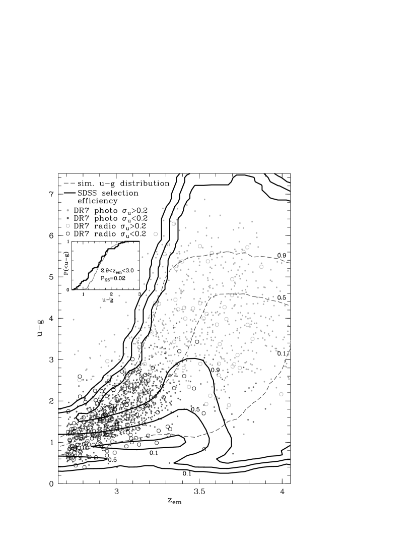
Figure 15.— Mock vs. observed $u-g$ quasar color as a function of redshift. Small filled circles (large open circles) show color-selected (radio-selected) $i<19.1$ quasars from the SDSS DR7 quasar catalog (Schneider et al., 2010). All plotted quasars have been selected by the final SDSS criteria (Richards et al., 2002). Quasars marginally detected in the $u$ band ($\sigma_{u}=0.2$ corresponds to S/N$\simeq 5$) are plotted in light gray. The dashed lines show the 10%, 50% and 90% percentiles of the $u-g$ color distribution of the simulated quasars. The solid contours show our derived SDSS selection efficiency at a given redshift and $u-g$ color. At $3.2\lesssim z_{\mathrm{em}}\lesssim 3.6$ blue ($u-g\lesssim 2$) quasars are missed by the SDSS color criteria, in contrast to radio-loud quasars selected independent of color. The lines in the inset compare the cumulative probability distributions of color-selected (thin) and radio-selected (thick) $2.9<z_{\mathrm{em}}<3$ SDSS quasars. The latter exhibit systematically bluer $u-g$ color than the former.

The thick contours in Fig. 15 show the SDSS selection efficiency at a given quasar redshift as a function of the $u-g$ color. At high redshifts ($z_{\mathrm{em}}\gtrsim 3.6$) the large range in color with a high selection efficiency means that almost all simulated quasars are selected regardless of their $u-g$ color. However, at $3\lesssim z_{\mathrm{em}}\lesssim 3.5$ the SDSS quasar targeting algorithm preferably selects red quasars and systematically misses blue ones. This color-dependent selection efficiency is in good agreement with the distribution of the observed color-selected SDSS quasars in Fig. 15. In particular, very few observed quasars have $u-g<1$ at $z_{\mathrm{em}}>3$, and most $z_{\mathrm{em}}\simeq 3.4$ SDSS quasars have $u-g>2$, leaving a prominent ’hole’ in color space compared to our predictions. On the other hand, the radio-selected SDSS quasars still reside in the color range of low selection efficiency. Our simulations also recover inhomogeneities in the color selection of $z_{\mathrm{em}}\lesssim 3$ quasars. Richards et al. (2002) define the ’mid-$z$’ inclusion box at $0.6<u-g<1.5$ with a targeting rate limited to 10% due to overlap with the stellar locus. However, candidates having $u-g<0.6$ are always followed up (this is the UV-excess criterion of Richards et al. 2002). Hence, there is a ’cluster’ of DR7 quasars at $u-g\simeq 0.6$ selected by UV excess, whereas at $0.7<u-g\lesssim 1$ there are very few color-selected quasars.

The color-dependent selection efficiency of SDSS is due to the difficulty to differentiate quasar colors from stellar colors. The blue quasars at $3\lesssim z_{\mathrm{em}}\lesssim 3.5$ do not separate well from the stellar locus, hence they are preferentially missed by the SDSS color selection criteria. But how does this explain the difference in the selection functions? Richards et al. (2006) used the IGM model by Fan (1999) that results in significantly redder $u-g$ colors and a high selection efficiency of $z_{\mathrm{em}}\gtrsim 3$ quasars and, therefore, in a higher predicted selection efficiency. An explicit color dependence of the selection efficiency complicates ’completeness’ corrections of color-based quasar surveys, rendering the average selection functions of Fig. 14 invalid. To illustrate this further, we plot in Fig. 14 the average selection function of simulated quasars with a measurable NUV flux ($m_{\mathrm{NUV}}<26$ including attenuation by the IGM). GALEX NUV-detected quasars are unusually blue in $u-g$, and consequently largely missed by the SDSS color selection criteria.

The inefficiency of SDSS to select high-redshift quasars with blue optical colors (and likely NUV flux) naturally explains why the Richards et al. (2006) selection function substantially overestimates the number counts of NUV-bright quasars in Fig. 13. Applying instead our color-dependent selection function lowers the prediction by almost a factor of 2. Unexpectedly, the predicted number counts are now in excellent agreement with the observed ones. In total, we predict $\sim 50$ SDSS quasars in the DR7 footprint that can be detected at S/N$>5$ in the NUV, very close to the actual 52 (58) with (without) flagging potential cases of source confusion. We predict slightly too many NUV-bright quasars at $21\lesssim m_{\mathrm{NUV}}\lesssim 22$, which may be due to the assumptions regarding the quasar UV spectral energy distribution or the LyC opacity (the MFP is extrapolated at $z<3.6$, Fig. 5).

5.3. The SDSS Lyman limit system bias revisited

Both, the observed differences in $u-g$ color of color-selected and radio-selected quasars and the good match of our strongly color-dependent selection function to observations, point to significant selection effects of SDSS, either regarding the quasars themselves, or the intergalactic absorption along their lines of sight. As all relevant spectral parameters of the model quasars and all IGM absorbers along their sightlines were saved in our MC simulations, we could explore both possibilities by comparing the statistical properties of the full MC sample and the subsample fulfilling the SDSS color selection criteria.

Indeed, we find that the median UV spectral index of SDSS-selected model quasars is larger at $z_{\mathrm{em}}<3.5$ (Fig. 16). The Gaussian distribution of spectral indices is well preserved, but the mean is shifted to higher values, yielding redder $u-g$ colors. Due to the increasing LyC opacity with redshift (see below), this bias decreases with increasing redshift. At $z_{\mathrm{em}}\simeq 2.7$ there is a sharp break in the UV spectral index distribution of quasars that would be selected by SDSS. This feature can be attributed to the inhomogeneities in the SDSS targeting rate in $u-g$ color space (Fig. 15). Blue $u-g$ colors can be due to hard UV spectral energy distributions, and the different targeting rates may cause non-trivial changes in the overall appearance of SDSS quasar spectra (e.g. composite spectra) as a function of redshift. The continuum redward of Ly$\alpha$ is not significantly biased considering our simple model assumptions. Nevertheless, the slight shift to a harder spectral index at $z_{\mathrm{em}}<3.5$ might indicate too stringent selection criteria in the other three SDSS colors. We conclude that SDSS preferentially selects $2.7\lesssim z_{\mathrm{em}}\lesssim 3.5$ quasars with red spectral energy distributions in the $u$ and $g$ band.

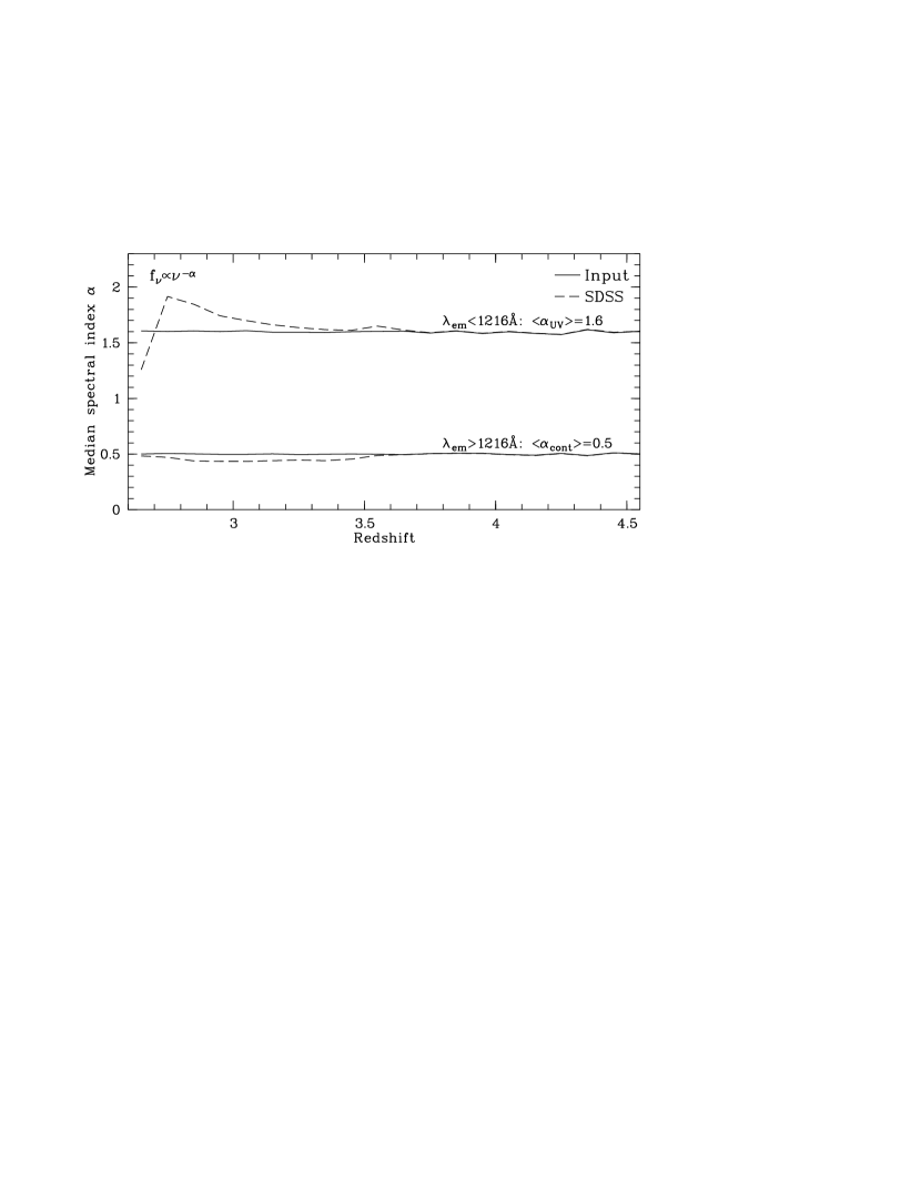
Figure 16.— Median spectral index $\alpha$ blueward and redward of H I Ly$\alpha$ as a function of redshift as adopted in the MC simulations (solid) and for the subset selected by the SDSS quasar targeting algorithm (dashed).

Lyman series and continuum absorption should have an even stronger impact on the $u-g$ color at these redshifts (Fig. 10). Therefore, we computed the mean IGM Lyman series and continuum transmission at different emission redshifts, both for the full sample of 4000 MC sightlines and for the subsample of sightlines towards quasars fulfilling the SDSS color selection criteria in a $\Delta z_{\mathrm{em}}=0.02$ window around the emission redshift of interest. The resulting average ’Lyman valley transmission spectra’ (e.g. Møller & Jakobsen, 1990) are plotted in Fig. 17. The sample of model spectra is large enough to clearly show the sawtooth-like features of overlapping Lyman series absorption. After an initial drop due to beginning series absorption at $z<z_{\mathrm{em}}$ the transmission recovers, because high-order high-redshift absorption overlaps with low-order low-redshift absorption that decreases with decreasing redshift. Beyond Ly$\epsilon$ there is a quasi-continuous roll-off of the transmission until LyC absorption sets in. At $z_{\mathrm{em}}=3.6$ there is essentially no difference between the average transmission of the full MC sample and SDSS-selected sightlines (compare the solid and dashed curves). However, at lower redshifts, the average LyC transmission towards SDSS-selected model sightlines is much lower than for general sightlines from the MC sample. The on average stronger LyC absorption corresponds to an on average redder $u-g$ color. Quasars at these redshifts are still in the vicinity of the stellar locus and LLSs in their sightlines will significantly redden the $u-g$ color, moving them away from the stellar locus so that they can be selected by broadband colors. On the other hand, quasars with little LyC absorption (e.g. without LLS) will have colors similar to main-sequence stars, and are preferentially missed by broadband color selection. Due to the rarity of LLSs, however, their excess towards SDSS quasars should not significantly bias the Ly$\alpha$ forest effective optical depth.

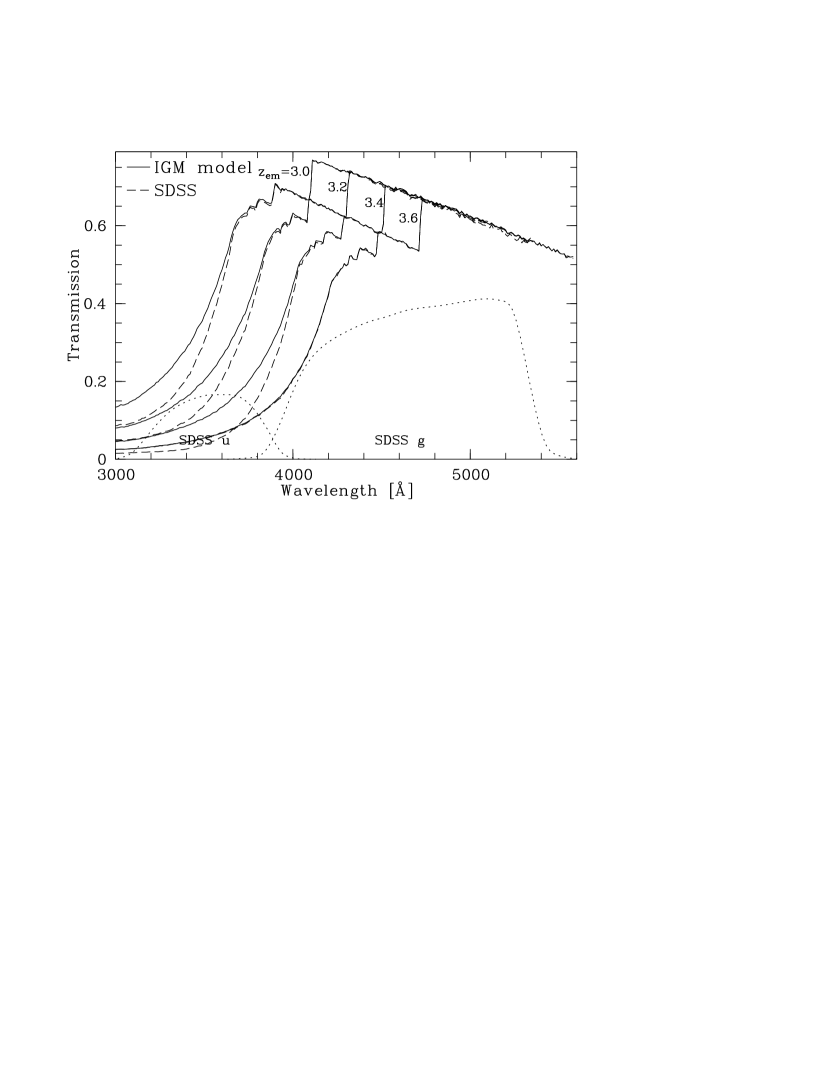
Figure 17.— Mean IGM Lyman series and continuum transmission for sources at $z_{\mathrm{em}}\in\left\{3.0,3.2,3.4,3.6\right\}$ from our 4000 MC simulations (solid) and for the subset selected by the SDSS quasar targeting algorithm (dashed). Each sawtooth curve is due to accumulating Lyman series absorption (first Ly$\alpha$, then Ly$\alpha$+Ly$\beta$, etc.), whereas the exponential-like roll-off is associated with the LyC opacity. Overplotted are the SDSS $u$ and $g$ filter curves (dotted).

Figure 17 presents further evidence that SDSS preferentially selects sightlines with strong H I absorbers at $z_{\mathrm{em}}<3.6$, an effect that plagued the interpretation of our previous results on the MFP and the number density of LLSs. In Prochaska et al. (2009) we found a significant flattening of the MFP at $z<3.6$ that coincides with an apparent overabundance of LLSs (Prochaska et al., 2010). We were puzzled that observed $z_{\mathrm{em}}\sim 3.5$ SDSS quasars are significantly redder than their brethren at $z_{\mathrm{em}}\sim 3.6$ and suspected that the SDSS color selection criteria had biased our measurements. The mock quasar spectra processed with the SDSS color selection routines support our previous claims. The SDSS-selected model quasars turn redder in $u-g$ towards lower redshifts, as only these red quasars are outliers from the stellar locus. At $3\lesssim z_{\mathrm{em}}\lesssim 3.5$ SDSS is essentially a Lyman break survey, resulting in an overabundance of LLSs and an underestimated MFP if the analysis is based solely on quasars from SDSS. Redder UV spectral indices of the quasars can alleviate this LLS bias somewhat, but not entirely.

6. Concluding remarks

We have correlated verified $z_{\mathrm{em}}>2.7$ quasars to GALEX photometry to reveal the rare high-redshift quasars whose far-UV fluxes are not extinguished by intervening Lyman limit systems, with the goal to establish a sample of UV-bright quasars that likely show intergalactic He II absorption. We have used the GALEX UV color $m_{\mathrm{FUV}}-m_{\mathrm{NUV}}$ to cull the most promising targets for follow-up. Red UV colors indicate that the quasar flux is prematurely truncated redward of the He II edge, whereas the rare quasars with blue UV colors and significant FUV flux will likely show flux at He II Ly$\alpha$.

We have performed extensive Monte Carlo simulations to estimate the UV color distribution of UV-bright quasars and their surface density on the sky. We predict that $\sim 600$ ($\sim 200$) quasars with $z_{\mathrm{em}}>2.7$ and $m_{1450}<19$ should be detectable in the NUV (FUV) at $m_{\mathrm{UV}}<21$ (Fig. 9; without considering sources near the Galactic plane). The number of UV-bright quasars strongly declines with redshift due to the declining quasar space density and the increasing H I Lyman continuum absorption experienced at the He II edge (Fig. 8). Nevertheless, there are enough targets within reach of HST/COS to significantly constrain He II reionization by He II absorption spectra, provided that the quasars are known and have been imaged with GALEX for efficient pre-selection.

Most confirmed $z_{\mathrm{em}}<3.5$ He II quasars have blue UV colors and our simulations indicate a $\sim 60$% He II detection rate of quasars at similar UV color (Fig. 12), a $\sim$50% increase over approaches that do not include color information (Syphers et al., 2009a, b). We have identified 166 additional quasars as prime targets for UV follow-up spectroscopy with HST/COS to significantly extend the sample of He II sightlines before the end of HST’s mission (Tables 3 and 4). We have started a survey with HST/COS in Cycle 17 to obtain FUV follow-up spectra of 8 UV-bright quasars selected from the much smaller GALEX GR3 footprint (star symbols in Fig. 12).

We have reassessed the SDSS color selection efficiency by applying the SDSS quasar selection criteria to mock photometry of our Monte Carlo spectra. We find that SDSS preferentially misses UV-bright quasars due to their blue colors that make them indistinguishable from main-sequence stars (Figs. 14 and 15). The observed $u-g$ colors of color-selected SDSS quasars are significantly redder than those of radio-selected ones at $3\lesssim z_{\mathrm{em}}\lesssim 3.5$, and agree well with our color-dependent SDSS selection function (Fig. 15). These missing quasars lack strong Lyman continuum absorption due to Lyman limit systems along their lines of sight that would redden the $u-g$ color (Fig. 17).

The SDSS color bias has not been well studied previously. Figure 18 of Bernardi et al. (2003) reveals that SDSS rarely selected blue quasars at $3.2<z_{\mathrm{em}}<3.6$, but the authors did not investigate this further. Richards et al. (2006) explored whether primarily radio-selected SDSS quasars have different color selection efficiencies, but due to low number statistics, they regarded the differences to be insignificant (their Fig. 10). For the first time we have been able to demonstrate the full effect and its consequences.

Since the UV-brightest quasars are among the bluest in SDSS $u-g$ at all epochs, we conclude that SDSS is inefficient in finding further promising targets for detecting intergalactic helium. Although about two dozen quasars in the SDSS database already have been confirmed to show He II (Syphers et al., 2009a, b), we predict that the FUV-brightest quasars without strong Lyman continuum absorption are insensitive to standard color selection techniques.

Due to the restrictive SDSS selection criteria the statistics of high-column density IGM absorbers measured towards color-selected SDSS quasars will be biased high (Prochaska et al., 2009, 2010). Our results also indicate that the incidence of DLAs based on SDSS samples (e.g Prochaska et al., 2005) has been overestimated. At $3\lesssim z_{\mathrm{em}}\lesssim 3.5$ the few radio-selected quasars are probably the only ones within SDSS that are truly unbiased in the statistics of high-column density absorbers.

The Lyman limit system bias will also affect the frequency of metal absorption lines that primarily occur at moderate to high H I column densities. Because these absorbers trace the large-scale structure of the IGM, the Lyman limit system bias might also impact analyses of the clustering properties and the power spectrum of the Ly$\alpha$ forest. Presumably all $z_{\mathrm{em}}\gtrsim 3$ quasars that have been first detected in broadband color surveys are affected by such a bias to some sort, depending on the exact color selection criteria and the number and effective wavelengths of the employed filters. Because the abundance of optically thick absorbers is far less constrained in reality than in ’completeness’ simulations like ours, determinations of the optical quasar luminosity function at $3<z_{\mathrm{em}}<3.5$ should invoke a variety of IGM models which will result in large systematic uncertainties in the luminosity function. Our study indicates that results based on color-selected high-redshift quasar samples are not as easy to interpret as previously thought due to the intertwined demographics of strong IGM absorbers and their background candles.

Table 3Promising targets to search for He II (GALEX S/N$>3$ and $m_{\mathrm{FUV}}-m_{\mathrm{NUV}}<1$).

Object	$\alpha$ (J2000)	$\delta$ (J2000)	$z_{\mathrm{em}}$	$m_{\mathrm{opt}}$	filter	$m_{\mathrm{FUV}}$ [AB]	$m_{\mathrm{NUV}}$ [AB]	limit	S/NFUV	S/NNUV	neighbors
2QZ J1411$-$0229	$14^{\mathrm{h}}11^{\mathrm{m}}24\fs 63$	$-02\arcdeg 29\arcmin 42\farcs 6$	$2.702$	$19.42$	$r$	$22.52$	$21.76$	0	5.3	9.1	0
FIRST J1007$+$4003	$10^{\mathrm{h}}07^{\mathrm{m}}16\fs 85$	$+40\arcdeg 03\arcmin 56\farcs 3$	$2.728$	$19.11$	$r$	$20.33$	$20.65$	0	4.6	5.3	0
SDSS J2330$+$0001	$23^{\mathrm{h}}30^{\mathrm{m}}26\fs 26$	$+00\arcdeg 01\arcmin 23\farcs 9$	$2.733$	$20.04$	$r$	$23.79$	$24.79$	0	12.3	5.5	3
CTS 0216	$02^{\mathrm{h}}16^{\mathrm{m}}23\fs 10$	$-39\arcdeg 07\arcmin 55\farcs 0$	$2.735$	$17.90$	$B$	$19.77$	$19.37$	0	5.2	11.9	2
SDSS J0029$+$0019	$00^{\mathrm{h}}29^{\mathrm{m}}12\fs 91$	$+00\arcdeg 19\arcmin 46\farcs 6$	$2.736$	$18.66$	$r$	$20.68$	$20.70$	0	25.6	28.7	1
SDSS J0142$-$0027	$01^{\mathrm{h}}42^{\mathrm{m}}43\fs 54$	$-00\arcdeg 27\arcmin 54\farcs 0$	$2.737$	$19.93$	$r$	$22.85$	$22.58$	0	4.1	5.2	0
SDSS J2358$-$0032	$23^{\mathrm{h}}58^{\mathrm{m}}07\fs 79$	$-00\arcdeg 32\arcmin 24\farcs 5$	$2.753$	$19.14$	$r$	$21.67$	$21.31$	0	9.9	16.7	0
UM 682	$03^{\mathrm{h}}10^{\mathrm{m}}28\fs 10$	$-19\arcdeg 09\arcmin 43\farcs 7$	$2.756$	$17.90$	$V$	$19.68$	$19.65$	0	7.2	11.6	2
PC 2204$+$0127	$22^{\mathrm{h}}06^{\mathrm{m}}46\fs 19$	$+01\arcdeg 41\arcmin 45\farcs 7$	$2.757$	$19.07$	$R$	$22.33$	$21.43$	0	5.0	12.0	2
PC 1640$+$4711	$16^{\mathrm{h}}41^{\mathrm{m}}25\fs 86$	$+47\arcdeg 05\arcmin 45\farcs 8$	$2.770$	$19.51$	$r$	$23.20$	$23.06$	0	4.0	4.8	0
SDSS J2324$-$0005	$23^{\mathrm{h}}24^{\mathrm{m}}52\fs 55$	$-00\arcdeg 05\arcmin 15\farcs 3$	$2.779$	$19.43$	$r$	$22.31$	$22.16$	0	31.1	32.9	3
SDSS J1309$-$0333	$13^{\mathrm{h}}09^{\mathrm{m}}34\fs 18$	$-03\arcdeg 33\arcmin 18\farcs 4$	$2.781$	$19.19$	$r$	$22.55$	$22.24$	0	5.6	6.8	0
SDSS J0809$+$3116	$08^{\mathrm{h}}09^{\mathrm{m}}12\fs 68$	$+31\arcdeg 16\arcmin 02\farcs 1$	$2.796$	$18.86$	$r$	$21.27$	$20.97$	0	3.1	6.7	0
Q 0207$-$398	$02^{\mathrm{h}}09^{\mathrm{m}}28\fs 59$	$-39\arcdeg 39\arcmin 39\farcs 5$	$2.805$	$17.15$	$V$	$20.29$	$21.07$	0	5.2	4.2	2
LBQS 1216$+$1656	$12^{\mathrm{h}}19^{\mathrm{m}}20\fs 40$	$+16\arcdeg 39\arcmin 29\farcs 5$	$2.818$	$18.17$	$r$	$20.80$	$20.04$	0	3.5	6.9	0
SDSS J1519$+$3609	$15^{\mathrm{h}}19^{\mathrm{m}}10\fs 37$	$+36\arcdeg 09\arcmin 40\farcs 5$	$2.819$	$18.70$	$r$	$20.87$	$20.59$	0	5.2	9.5	0
Q 2315$-$4230	$23^{\mathrm{h}}18^{\mathrm{m}}15\fs 10$	$-42\arcdeg 13\arcmin 48\farcs 0$	$2.830$	$20.00$	$V$	$21.94$	$21.37$	0	11.6	21.0	2
SDSS J1230$-$0253	$12^{\mathrm{h}}30^{\mathrm{m}}53\fs 16$	$-02\arcdeg 53\arcmin 52\farcs 0$	$2.837$	$18.92$	$r$	$21.88$	$23.30$	0	7.0	3.3	0
2QZ J2158$-$3037	$21^{\mathrm{h}}58^{\mathrm{m}}29\fs 66$	$-30\arcdeg 37\arcmin 21\farcs 6$	$2.838$	$20.35$	$b_{J}$	$24.57$	$24.61$	1	3.9	3.3	3
HS 1024$+$1849	$10^{\mathrm{h}}27^{\mathrm{m}}34\fs 13$	$+18\arcdeg 34\arcmin 27\farcs 5$	$2.840$	$17.83$	$r$	$19.97$	$19.82$	0	5.3	16.9	0
SDSS J0141$+$1341	$01^{\mathrm{h}}41^{\mathrm{m}}34\fs 01$	$+13\arcdeg 41\arcmin 58\farcs 9$	$2.843$	$19.52$	$r$	$22.95$	$22.76$	0	3.5	5.8	0
SDSS J2156$+$0037	$21^{\mathrm{h}}56^{\mathrm{m}}04\fs 18$	$+00\arcdeg 37\arcmin 42\farcs 3$	$2.844$	$19.01$	$r$	$21.90$	$21.39$	0	9.2	13.3	1
CSO 0806	$13^{\mathrm{h}}04^{\mathrm{m}}11\fs 99$	$+29\arcdeg 53\arcmin 48\farcs 8$	$2.850$	$17.65$	$r$	$20.46$	$20.47$	0	15.9	26.1	0
SDSS J2331$+$0036	$23^{\mathrm{h}}31^{\mathrm{m}}31\fs 48$	$+00\arcdeg 36\arcmin 44\farcs 4$	$2.852$	$19.53$	$r$	$22.55$	$21.96$	0	4.1	5.3	0
SBS 1602$+$576	$16^{\mathrm{h}}03^{\mathrm{m}}55\fs 92$	$+57\arcdeg 30\arcmin 54\farcs 4$	$2.858$	$17.33$	$r$	$19.76$	$19.08$	0	8.2	16.1	0
PMN J1404$+$0728	$14^{\mathrm{h}}04^{\mathrm{m}}32\fs 99$	$+07\arcdeg 28\arcmin 46\farcs 9$	$2.866$	$18.87$	$r$	$20.78$	$21.29$	0	4.0	3.7	0
PC 0058$+$0215	$01^{\mathrm{h}}00^{\mathrm{m}}58\fs 40$	$+02\arcdeg 31\arcmin 32\farcs 0$	$2.868$	$18.91$	$R$	$21.32$	$21.22$	0	6.4	7.4	2
CTS 0347	$22^{\mathrm{h}}05^{\mathrm{m}}36\fs 26$	$-34\arcdeg 26\arcmin 03\farcs 9$	$2.870$	$18.70$	$R$	$20.89$	$20.48$	0	5.4	7.9	2
2QZ J0126$-$3124	$01^{\mathrm{h}}26^{\mathrm{m}}00\fs 17$	$-31\arcdeg 24\arcmin 21\farcs 5$	$2.881$	$20.43$	$b_{J}$	$21.48$	$22.84$	0	4.6	3.0	2
SDSS J1626$+$3856	$16^{\mathrm{h}}26^{\mathrm{m}}12\fs 99$	$+38\arcdeg 56\arcmin 27\farcs 2$	$2.882$	$18.63$	$r$	$21.23$	$21.82$	0	3.2	3.1	0
SDSS J2342$-$0042	$23^{\mathrm{h}}42^{\mathrm{m}}36\fs 90$	$-00\arcdeg 42\arcmin 32\farcs 8$	$2.885$	$20.47$	$r$	$24.06$	$23.21$	0	4.6	4.2	0
SDSS J1410$+$4727	$14^{\mathrm{h}}10^{\mathrm{m}}59\fs 61$	$+47\arcdeg 27\arcmin 33\farcs 3$	$2.901$	$19.38$	$r$	$21.74$	$21.31$	0	3.1	5.2	0
SDSS J1443$+$3546	$14^{\mathrm{h}}43^{\mathrm{m}}11\fs 58$	$+35\arcdeg 46\arcmin 46\farcs 3$	$2.941$	$18.79$	$r$	$20.96$	$21.19$	0	4.3	4.6	0
RDS 477A	$10^{\mathrm{h}}53^{\mathrm{m}}06\fs 04$	$+57\arcdeg 34\arcmin 24\farcs 6$	$2.949$	$20.47$	$r$	$24.55$	$24.51$	0	3.1	3.6	3
SDSS J0818$+$4908	$08^{\mathrm{h}}18^{\mathrm{m}}50\fs 01$	$+49\arcdeg 08\arcmin 17\farcs 0$	$2.954$	$18.52$	$r$	$21.49$	$21.46$	0	11.6	22.6	0
SDSS J1033$+$5406	$10^{\mathrm{h}}33^{\mathrm{m}}10\fs 71$	$+54\arcdeg 06\arcmin 46\farcs 8$	$2.959$	$19.27$	$r$	$22.55$	$23.13$	0	4.9	4.4	0
FIRST J1456$-$0218	$14^{\mathrm{h}}56^{\mathrm{m}}40\fs 98$	$-02\arcdeg 18\arcmin 19\farcs 4$	$2.963$	$19.53$	$r$	$22.80$	$22.07$	0	4.5	7.4	0
SDSS J0922$+$5321	$09^{\mathrm{h}}22^{\mathrm{m}}47\fs 83$	$+53\arcdeg 21\arcmin 46\farcs 6$	$3.000$	$19.75$	$r$	$22.76$	$23.32$	0	4.1	3.4	0
SDSS J1657$+$3553	$16^{\mathrm{h}}57^{\mathrm{m}}51\fs 68$	$+35\arcdeg 53\arcmin 18\farcs 0$	$3.005$	$19.23$	$r$	$23.35$	$22.81$	0	5.2	7.4	0
SDSS J0905$+$3057	$09^{\mathrm{h}}05^{\mathrm{m}}08\fs 88$	$+30\arcdeg 57\arcmin 57\farcs 3$	$3.027$	$17.37$	$r$	$20.89$	$21.62$	0	6.5	5.5	0
SDSS J1101$+$1053	$11^{\mathrm{h}}01^{\mathrm{m}}55\fs 73$	$+10\arcdeg 53\arcmin 02\farcs 3$	$3.031$	$18.97$	$r$	$21.59$	$21.94$	0	4.0	4.0	0
SDSS J1244$+$6201	$12^{\mathrm{h}}44^{\mathrm{m}}56\fs 98$	$+62\arcdeg 01\arcmin 43\farcs 0$	$3.057$	$18.63$	$r$	$21.08$	$21.33$	0	4.7	7.8	0
SDSS J1052$+$2543	$10^{\mathrm{h}}52^{\mathrm{m}}54\fs 49$	$+25\arcdeg 43\arcmin 03\farcs 9$	$3.062$	$18.52$	$r$	$21.43$	$20.96$	0	3.1	3.9	0
PC 2211$+$0119	$22^{\mathrm{h}}14^{\mathrm{m}}27\fs 81$	$+01\arcdeg 34\arcmin 57\farcs 3$	$3.100$	$19.10$	$R$	$22.26$	$22.35$	0	5.4	6.7	2
SDSS J1025$+$0452	$10^{\mathrm{h}}25^{\mathrm{m}}09\fs 63$	$+04\arcdeg 52\arcmin 46\farcs 7$	$3.244$	$18.02$	$r$	$21.37$	$21.72$	0	3.8	3.1	0
SDSS J0955$+$6842	$09^{\mathrm{h}}55^{\mathrm{m}}54\fs 30$	$+68\arcdeg 42\arcmin 01\farcs 2$	$3.269$	$19.26$	$r$	$24.05$	$24.06$	0	5.4	6.1	3
SDSS J1220$+$4549	$12^{\mathrm{h}}20^{\mathrm{m}}17\fs 06$	$+45\arcdeg 49\arcmin 41\farcs 1$	$3.293$	$18.20$	$r$	$22.78$	$22.83$	0	3.8	5.7	0
HS 0911$+$4809	$09^{\mathrm{h}}15^{\mathrm{m}}10\fs 01$	$+47\arcdeg 56\arcmin 58\farcs 7$	$3.337$	$17.84$	$r$	$20.53$	$20.25$	0	5.3	9.4	0
SDSS J0054$+$0028	$00^{\mathrm{h}}54^{\mathrm{m}}01\fs 48$	$+00\arcdeg 28\arcmin 47\farcs 7$	$3.413$	$19.93$	$r$	$22.06$	$21.79$	0	7.6	8.6	1
CLASXS 449	$10^{\mathrm{h}}34^{\mathrm{m}}58\fs 01$	$+57\arcdeg 50\arcmin 46\farcs 5$	$3.430$	$23.80$	$R$	$24.19$	$23.63$	0	4.5	6.1	0
SDSS J1233$+$0941	$12^{\mathrm{h}}33^{\mathrm{m}}02\fs 74$	$+09\arcdeg 41\arcmin 44\farcs 2$	$3.816$	$20.36$	$r$	$23.66$	$23.03$	0	3.7	3.4	0
CDFN 097	$12^{\mathrm{h}}36^{\mathrm{m}}12\fs 93$	$+62\arcdeg 19\arcmin 29\farcs 8$	$3.938$	$22.80$	$R$	$25.78$	$24.97$	0	4.5	5.3	0

Note. — 39 of the 41 $z_{\mathrm{em}}>2.78$ quasars were previously suggested as candidate He II quasars by Syphers et al. (2009a).

Table 4Further quasars with potential FUV flux (GALEX S/N${}_{\mathrm{FUV}}>2$).

Object	$\alpha$ (J2000)	$\delta$ (J2000)	$z_{\mathrm{em}}$	$m_{\mathrm{opt}}$	filter	$m_{\mathrm{FUV}}$ [AB]	$m_{\mathrm{NUV}}$ [AB]	limit	S/NFUV	S/NNUV	neighbors
2QZ J0035$-$2837	$00^{\mathrm{h}}35^{\mathrm{m}}24\fs 23$	$-28\arcdeg 37\arcmin 14\farcs 7$	$2.702$	$20.73$	$b_{J}$	$22.70$	$22.27$	0	2.2	2.6	2
2QZ J0258$-$2941	$02^{\mathrm{h}}58^{\mathrm{m}}09\fs 15$	$-29\arcdeg 41\arcmin 08\farcs 7$	$2.702$	$20.12$	$b_{J}$	$21.78$	$22.43$	0	3.5	2.8	2
SDSS J1039$+$3040	$10^{\mathrm{h}}39^{\mathrm{m}}24\fs 05$	$+30\arcdeg 40\arcmin 59\farcs 5$	$2.705$	$19.99$	$r$	$21.96$	$23.78$	2	2.9	0.7	0
SDSS J1301$-$0038	$13^{\mathrm{h}}01^{\mathrm{m}}47\fs 88$	$-00\arcdeg 38\arcmin 17\farcs 3$	$2.705$	$19.40$	$r$	$22.99$	$24.47$	2	2.4	0	0
2QZ J2153$-$2719	$21^{\mathrm{h}}53^{\mathrm{m}}16\fs 08$	$-27\arcdeg 19\arcmin 38\farcs 6$	$2.706$	$20.04$	$b_{J}$	$22.14$	$21.59$	0	2.5	3.8	2
2QZ J0203$-$3153	$02^{\mathrm{h}}03^{\mathrm{m}}15\fs 58$	$-31\arcdeg 53\arcmin 54\farcs 9$	$2.710$	$20.65$	$b_{J}$	$22.21$	$20.95$	2	2.5	2.0	2
CTS 0538	$14^{\mathrm{h}}21^{\mathrm{m}}01\fs 60$	$-23\arcdeg 07\arcmin 32\farcs 0$	$2.710$	$18.50$	$R$	$21.31$	$21.35$	0	2.7	3.0	2
SDSS J1407$+$2127	$14^{\mathrm{h}}07^{\mathrm{m}}01\fs 12$	$+21\arcdeg 27\arcmin 15\farcs 9$	$2.711$	$18.35$	$r$	$21.86$	$20.88$	0	2.2	6.8	0
SDSS J1325$+$0814	$13^{\mathrm{h}}25^{\mathrm{m}}17\fs 85$	$+08\arcdeg 14\arcmin 08\farcs 4$	$2.715$	$18.70$	$r$	$22.31$	$22.69$	0	2.8	2.5	0
SDSS J0014$-$0112	$00^{\mathrm{h}}14^{\mathrm{m}}43\fs 69$	$-01\arcdeg 12\arcmin 06\farcs 4$	$2.717$	$18.84$	$r$	$23.99$	$21.76$	0	3.7	12.3	0
Q 0040$-$370	$00^{\mathrm{h}}42^{\mathrm{m}}43\fs 93$	$-36\arcdeg 47\arcmin 41\farcs 5$	$2.723$	$17.85$	$V$	$21.30$	$21.33$	0	2.8	3.8	2
2QZ J0141$-$3209	$01^{\mathrm{h}}41^{\mathrm{m}}54\fs 69$	$-32\arcdeg 09\arcmin 11\farcs 6$	$2.724$	$20.03$	$b_{J}$	$22.77$	$22.20$	2	2.3	4.3	2
SDSS J1159$+$0222	$11^{\mathrm{h}}59^{\mathrm{m}}04\fs 30$	$+02\arcdeg 22\arcmin 14\farcs 1$	$2.725$	$19.11$	$r$	$22.40$	$21.10$	1	3.5	10.7	0
Q 1613$+$172	$16^{\mathrm{h}}15^{\mathrm{m}}56\fs 87$	$+17\arcdeg 07\arcmin 51\farcs 4$	$2.729$	$18.24$	$r$	$22.00$	$22.78$	0	2.8	2.5	0
QSO J0059$-$3541	$00^{\mathrm{h}}59^{\mathrm{m}}14\fs 21$	$-35\arcdeg 41\arcmin 42\farcs 1$	$2.730$	$18.04$	$V$	$22.24$	$20.97$	0	6.3	16.4	2
SDSS J1026$+$2842	$10^{\mathrm{h}}26^{\mathrm{m}}54\fs 39$	$+28\arcdeg 42\arcmin 54\farcs 5$	$2.739$	$19.68$	$r$	$22.62$	$22.09$	0	2.2	3.7	0
HE 0151$-$4326	$01^{\mathrm{h}}53^{\mathrm{m}}27\fs 20$	$-43\arcdeg 11\arcmin 38\farcs 0$	$2.740$	$17.19$	$b_{J}$	$20.63$	$19.30$	0	5.8	15.5	2
2QZ J1129$+$0134	$11^{\mathrm{h}}29^{\mathrm{m}}57\fs 65$	$+01\arcdeg 34\arcmin 16\farcs 0$	$2.743$	$19.74$	$r$	$22.35$	$22.49$	1	2.2	2.7	1
2QZ J1326$+$0042	$13^{\mathrm{h}}26^{\mathrm{m}}22\fs 41$	$+00\arcdeg 42\arcmin 37\farcs 3$	$2.743$	$18.72$	$r$	$21.66$	$21.65$	0	2.7	3.4	0
2QZ J0053$-$3140	$00^{\mathrm{h}}53^{\mathrm{m}}30\fs 68$	$-31\arcdeg 40\arcmin 18\farcs 8$	$2.751$	$19.99$	$b_{J}$	$23.67$	$21.87$	0	2.1	7.1	2
2QZ J0012$-$3131	$00^{\mathrm{h}}12^{\mathrm{m}}43\fs 11$	$-31\arcdeg 31\arcmin 13\farcs 6$	$2.755$	$19.84$	$b_{J}$	$22.64$	$22.35$	1	2.2	3.2	2
HELLAS 149	$20^{\mathrm{h}}44^{\mathrm{m}}34\fs 80$	$-10\arcdeg 28\arcmin 08\farcs 0$	$2.755$	$17.79$	$V$	$21.34$	$20.15$	0	3.7	8.0	2
QSO J0056$-$4013	$00^{\mathrm{h}}56^{\mathrm{m}}11\fs 76$	$-40\arcdeg 13\arcmin 16\farcs 2$	$2.758$	$18.10$	$R$	$21.58$	$23.15$	0	2.7	2.2	2
SDSS J1600$+$4033	$16^{\mathrm{h}}00^{\mathrm{m}}33\fs 09$	$+40\arcdeg 33\arcmin 43\farcs 9$	$2.761$	$19.20$	$r$	$22.28$	$21.58$	1	2.4	6.1	0
SDSS J0150$-$0825	$01^{\mathrm{h}}50^{\mathrm{m}}09\fs 46$	$-08\arcdeg 25\arcmin 10\farcs 8$	$2.763$	$18.96$	$r$	$23.64$	$23.29$	0	2.7	3.4	0
SDSS J0809$+$0658	$08^{\mathrm{h}}09^{\mathrm{m}}46\fs 14$	$+06\arcdeg 58\arcmin 07\farcs 9$	$2.763$	$20.04$	$r$	$24.17$	$24.01$	1	2.1	2.4	0
SDSS J1546$+$2315	$15^{\mathrm{h}}46^{\mathrm{m}}59\fs 33$	$+23\arcdeg 15\arcmin 47\farcs 3$	$2.777$	$17.80$	$r$	$22.22$	$22.65$	1	2.3	2.9	0
2QZ J0034$-$3048	$00^{\mathrm{h}}34^{\mathrm{m}}47\fs 21$	$-30\arcdeg 48\arcmin 13\farcs 5$	$2.785$	$19.97$	$b_{J}$	$22.59$	$21.46$	0	2.7	6.4	2
SDSS J1418$+$5858	$14^{\mathrm{h}}18^{\mathrm{m}}22\fs 89$	$+58\arcdeg 58\arcmin 06\farcs 4$	$2.785$	$17.78$	$r$	$21.74$	$19.94$	0	2.3	11.7	0
LBQS 0041$-$2707	$00^{\mathrm{h}}43^{\mathrm{m}}51\fs 83$	$-26\arcdeg 51\arcmin 27\farcs 5$	$2.786$	$17.83$	$V$	$21.79$	$22.01$	0	3.3	3.0	2
2QZ J0044$-$3147	$00^{\mathrm{h}}44^{\mathrm{m}}05\fs 04$	$-31\arcdeg 47\arcmin 04\farcs 5$	$2.789$	$19.80$	$b_{J}$	$22.66$	$22.27$	0	2.7	5.5	2
2QZ J2223$-$3131	$22^{\mathrm{h}}23^{\mathrm{m}}12\fs 45$	$-31\arcdeg 31\arcmin 29\farcs 4$	$2.792$	$19.44$	$b_{J}$	$22.07$	$22.59$	0	2.8	2.8	2
SDSS J0103$+$0026	$01^{\mathrm{h}}03^{\mathrm{m}}37\fs 46$	$+00\arcdeg 26\arcmin 08\farcs 2$	$2.795$	$20.35$	$r$	$23.54$	$25.65$	2	4.4	0	0
2QZ J1428$+$0010	$14^{\mathrm{h}}28^{\mathrm{m}}49\fs 85$	$+00\arcdeg 10\arcmin 40\farcs 7$	$2.807$	$19.79$	$r$	$21.65$	$23.60$	2	2.2	0	0
H 0853$+$1953	$08^{\mathrm{h}}56^{\mathrm{m}}26\fs 47$	$+19\arcdeg 41\arcmin 37\farcs 7$	$2.818$	$18.74$	$r$	$23.31$	$22.17$	0	3.8	6.5	0
SDSS J0225$+$0048	$02^{\mathrm{h}}25^{\mathrm{m}}19\fs 50$	$+00\arcdeg 48\arcmin 23\farcs 6$	$2.820$	$20.54$	$r$	$24.82$	$23.01$	0	2.4	5.7	0
SDSS J0030$+$0053	$00^{\mathrm{h}}30^{\mathrm{m}}17\fs 11$	$+00\arcdeg 53\arcmin 58\farcs 8$	$2.831$	$19.92$	$r$	$23.78$	$24.34$	0	3.3	2.4	0
FIRST J0905$+$3555	$09^{\mathrm{h}}05^{\mathrm{m}}36\fs 07$	$+35\arcdeg 55\arcmin 51\farcs 6$	$2.839$	$18.39$	$r$	$21.88$	$21.60$	0	2.3	3.2	0
SDSS J1504$-$0008	$15^{\mathrm{h}}04^{\mathrm{m}}25\fs 53$	$-00\arcdeg 08\arcmin 03\farcs 2$	$2.840$	$18.92$	$r$	$22.44$	$23.94$	2	3.9	0.9	0
2QZ J0024$-$3149	$00^{\mathrm{h}}24^{\mathrm{m}}16\fs 22$	$-31\arcdeg 49\arcmin 42\farcs 9$	$2.846$	$20.24$	$b_{J}$	$22.56$	$22.36$	0	2.6	3.0	2
UM 658	$22^{\mathrm{h}}46^{\mathrm{m}}52\fs 66$	$-22\arcdeg 03\arcmin 09\farcs 2$	$2.852$	$17.80$	$V$	$22.40$	$21.80$	0	2.3	2.5	2
SDSS J0034$-$0109	$00^{\mathrm{h}}34^{\mathrm{m}}20\fs 62$	$-01\arcdeg 09\arcmin 17\farcs 3$	$2.854$	$20.24$	$r$	$23.73$	$22.55$	0	3.6	6.5	0
SDSS J1309$+$2815	$13^{\mathrm{h}}09^{\mathrm{m}}39\fs 49$	$+28\arcdeg 15\arcmin 08\farcs 0$	$2.854$	$18.99$	$r$	$21.71$	$23.17$	2	2.7	0.1	0
SDSS J1439$+$0421	$14^{\mathrm{h}}39^{\mathrm{m}}48\fs 06$	$+04\arcdeg 21\arcmin 12\farcs 8$	$2.857$	$19.00$	$r$	$23.99$	$24.16$	0	2.6	2.2	0
SDSS J1241$+$2719	$12^{\mathrm{h}}41^{\mathrm{m}}40\fs 98$	$-27\arcdeg 19\arcmin 27\farcs 5$	$2.862$	$19.21$	$r$	$22.54$	$23.86$	2	2.0	1.1	0
SDSS J0039$+$1527	$00^{\mathrm{h}}39^{\mathrm{m}}39\fs 96$	$+15\arcdeg 27\arcmin 20\farcs 3$	$2.867$	$19.14$	$r$	$23.04$	$23.99$	2	4.0	1.9	0
FIRST J1231$+$0102	$12^{\mathrm{h}}31^{\mathrm{m}}39\fs 12$	$+01\arcdeg 02\arcmin 29\farcs 3$	$2.883$	$18.33$	$r$	$22.67$	$20.57$	0	3.9	26.2	0
SDSS J1154$+$4030	$11^{\mathrm{h}}54^{\mathrm{m}}13\fs 87$	$+40\arcdeg 30\arcmin 00\farcs 1$	$2.893$	$20.36$	$r$	$21.64$	$23.27$	2	2.4	1.0	0
SDSS J0130$-$0007	$01^{\mathrm{h}}30^{\mathrm{m}}43\fs 41$	$-00\arcdeg 07\arcmin 35\farcs 3$	$2.894$	$19.95$	$r$	$23.76$	$23.57$	0	2.8	2.2	0
2QZ J0114$-$2719	$01^{\mathrm{h}}14^{\mathrm{m}}19\fs 16$	$-27\arcdeg 19\arcmin 12\farcs 4$	$2.896$	$20.55$	$b_{J}$	$22.64$	$23.30$	2	2.6	2.1	2
SDSS J1322$+$3955	$13^{\mathrm{h}}22^{\mathrm{m}}59\fs 97$	$+39\arcdeg 55\arcmin 29\farcs 9$	$2.898$	$18.35$	$r$	$22.19$	$23.10$	0	3.4	2.7	0
SDSS J1427$+$0014	$14^{\mathrm{h}}27^{\mathrm{m}}09\fs 81$	$+00\arcdeg 14\arcmin 50\farcs 2$	$2.908$	$18.54$	$r$	$23.56$	$23.32$	0	2.6	2.8	0
PKS 0246$-$231	$02^{\mathrm{h}}48^{\mathrm{m}}22\fs 74$	$-22\arcdeg 57\arcmin 58\farcs 2$	$2.914$	$20.00$	$R$	$22.15$	$21.42$	0	2.3	3.1	2
SDSS J1525$+$2207	$15^{\mathrm{h}}25^{\mathrm{m}}34\fs 50$	$+22\arcdeg 07\arcmin 00\farcs 7$	$2.914$	$19.12$	$r$	$21.92$	$21.87$	0	2.6	2.8	1
SDSS J1210$+$3509	$12^{\mathrm{h}}10^{\mathrm{m}}40\fs 36$	$+35\arcdeg 09\arcmin 11\farcs 3$	$2.919$	$19.87$	$r$	$22.59$	$21.72$	1	2.1	5.1	0
FIRST J0936$+$2927	$09^{\mathrm{h}}36^{\mathrm{m}}43\fs 51$	$+29\arcdeg 27\arcmin 13\farcs 6$	$2.926$	$18.11$	$r$	$20.80$	$20.59$	0	3.0	4.7	0
SDSS J0300$-$0749	$03^{\mathrm{h}}00^{\mathrm{m}}47\fs 62$	$-07\arcdeg 49\arcmin 02\farcs 8$	$2.939$	$20.02$	$r$	$22.84$	$21.73$	0	3.7	4.3	0
FIRST J1604$+$1645	$16^{\mathrm{h}}04^{\mathrm{m}}41\fs 47$	$+16\arcdeg 45\arcmin 38\farcs 3$	$2.939$	$16.68$	$r$	$21.01$	$19.56$	0	4.7	16.2	0
FIRST J1159$+$4136	$11^{\mathrm{h}}59^{\mathrm{m}}47\fs 10$	$+41\arcdeg 36\arcmin 59\farcs 1$	$2.944$	$18.71$	$r$	$22.12$	$21.93$	0	2.6	4.2	0
FIRST J1332$+$0805	$13^{\mathrm{h}}32^{\mathrm{m}}18\fs 55$	$+08\arcdeg 05\arcmin 48\farcs 3$	$2.947$	$18.86$	$r$	$21.90$	$23.73$	2	2.6	0	1
SDSS J0905$+$4107	$09^{\mathrm{h}}05^{\mathrm{m}}18\fs 02$	$+41\arcdeg 07\arcmin 57\farcs 6$	$2.954$	$19.70$	$r$	$22.56$	$23.01$	1	2.0	1.8	1
QSO J1334$+$2801	$13^{\mathrm{h}}34^{\mathrm{m}}36\fs 63$	$+28\arcdeg 01\arcmin 41\farcs 5$	$2.958$	$19.17$	$r$	$22.17$	$23.85$	2	2.1	0.3	0
SDSS J1143$+$3017	$11^{\mathrm{h}}43^{\mathrm{m}}14\fs 67$	$+30\arcdeg 17\arcmin 11\farcs 8$	$2.964$	$18.89$	$r$	$21.66$	$23.43$	2	2.5	0	0
SDSS J2039$-$0047	$20^{\mathrm{h}}39^{\mathrm{m}}06\fs 09$	$-00\arcdeg 47\arcmin 36\farcs 6$	$2.966$	$19.46$	$r$	$23.40$	$26.03$	2	3.2	0.5	0
SDSS J1335$+$2230	$13^{\mathrm{h}}35^{\mathrm{m}}03\fs 67$	$+22\arcdeg 30\arcmin 52\farcs 7$	$2.972$	$18.95$	$r$	$21.42$	$21.43$	0	2.7	3.2	0
SDSS J1356$+$0556	$13^{\mathrm{h}}56^{\mathrm{m}}20\fs 83$	$+05\arcdeg 56\arcmin 19\farcs 7$	$2.973$	$19.03$	$r$	$21.73$	$21.77$	0	2.6	2.4	0
2QZ J0239$-$2749	$02^{\mathrm{h}}39^{\mathrm{m}}23\fs 60$	$-27\arcdeg 49\arcmin 30\farcs 8$	$2.982$	$20.11$	$b_{J}$	$23.46$	$25.07$	2	3.3	0.5	2
SDSS J2310$+$0048	$23^{\mathrm{h}}10^{\mathrm{m}}55\fs 32$	$+00\arcdeg 48\arcmin 17\farcs 1$	$2.993$	$18.71$	$r$	$22.66$	$21.44$	0	5.5	12.2	0
2QZ J2343$-$2947	$23^{\mathrm{h}}43^{\mathrm{m}}35\fs 21$	$-29\arcdeg 47\arcmin 00\farcs 6$	$2.995$	$19.65$	$b_{J}$	$22.27$	$22.08$	0	2.4	4.4	2
SDSS J1311$+$0857	$13^{\mathrm{h}}11^{\mathrm{m}}27\fs 42$	$+08\arcdeg 57\arcmin 15\farcs 0$	$3.009$	$19.19$	$r$	$21.64$	$23.82$	2	2.3	0	0
SDSS J1040$+$2446	$10^{\mathrm{h}}40^{\mathrm{m}}03\fs 62$	$+24\arcdeg 46\arcmin 53\farcs 0$	$3.012$	$19.46$	$r$	$22.25$	$22.11$	0	2.3	2.1	0
SDSS J0858$+$4012	$08^{\mathrm{h}}58^{\mathrm{m}}33\fs 02$	$+40\arcdeg 12\arcmin 03\farcs 1$	$3.013$	$18.81$	$r$	$22.35$	$22.87$	1	2.4	2.4	0
SDSS J1146$+$2306	$11^{\mathrm{h}}46^{\mathrm{m}}09\fs 81$	$+23\arcdeg 06\arcmin 13\farcs 7$	$3.013$	$18.94$	$r$	$21.44$	$21.13$	0	2.6	3.7	0
SDSS J2334$-$1039	$23^{\mathrm{h}}34^{\mathrm{m}}49\fs 48$	$-10\arcdeg 39\arcmin 41\farcs 0$	$3.019$	$19.96$	$r$	$23.14$	$23.76$	0	4.0	2.2	1
SDSS J0924$+$4852	$09^{\mathrm{h}}24^{\mathrm{m}}47\fs 35$	$+48\arcdeg 52\arcmin 42\farcs 8$	$3.020$	$18.31$	$r$	$21.60$	$21.19$	0	2.8	4.1	0
SDSS J0947$+$1421	$09^{\mathrm{h}}47^{\mathrm{m}}34\fs 19$	$+14\arcdeg 21\arcmin 16\farcs 9$	$3.030$	$17.22$	$r$	$20.94$	$19.70$	0	4.2	9.3	0
SDSS J1630$+$4145	$16^{\mathrm{h}}30^{\mathrm{m}}05\fs 72$	$+41\arcdeg 45\arcmin 09\farcs 1$	$3.033$	$19.53$	$r$	$21.20$	$22.71$	2	3.0	2.2	0
SDSS J1159$+$3134	$11^{\mathrm{h}}59^{\mathrm{m}}11\fs 52$	$+31\arcdeg 34\arcmin 27\farcs 3$	$3.055$	$17.70$	$r$	$21.91$	$21.35$	0	2.4	3.6	0
FIRST J0921$+$3051	$09^{\mathrm{h}}21^{\mathrm{m}}56\fs 27$	$+30\arcdeg 51\arcmin 57\farcs 1$	$3.062$	$18.75$	$r$	$21.63$	$23.94$	2	2.8	0.2	0
SDSS J1430$+$2307	$14^{\mathrm{h}}30^{\mathrm{m}}06\fs 11$	$+23\arcdeg 07\arcmin 21\farcs 4$	$3.062$	$20.16$	$r$	$21.54$	$22.46$	0	2.4	2.9	0
SDSS J1225$+$1933	$12^{\mathrm{h}}25^{\mathrm{m}}45\fs 89$	$+19\arcdeg 33\arcmin 41\farcs 3$	$3.066$	$19.30$	$r$	$21.45$	$21.54$	0	3.0	3.3	0
PMN J1458$+$0855	$14^{\mathrm{h}}58^{\mathrm{m}}05\fs 99$	$+08\arcdeg 55\arcmin 30\farcs 1$	$3.066$	$20.27$	$r$	$22.04$	$23.27$	2	2.4	1.3	0
SDSS J1207$+$3509	$12^{\mathrm{h}}07^{\mathrm{m}}06\fs 99$	$+35\arcdeg 09\arcmin 22\farcs 2$	$3.094$	$19.77$	$r$	$21.78$	$22.19$	0	2.3	3.8	1
SDSS J1644$+$2143	$16^{\mathrm{h}}44^{\mathrm{m}}39\fs 86$	$+21\arcdeg 43\arcmin 11\farcs 5$	$3.111$	$18.43$	$r$	$21.60$	$21.90$	1	2.5	2.9	1
SDSS J1259$+$6355	$12^{\mathrm{h}}59^{\mathrm{m}}48\fs 78$	$+63\arcdeg 55\arcmin 36\farcs 9$	$3.114$	$19.32$	$r$	$21.90$	$22.65$	2	2.2	1.9	0
SDSS J1215$+$3138	$12^{\mathrm{h}}15^{\mathrm{m}}57\fs 28$	$+31\arcdeg 38\arcmin 41\farcs 4$	$3.120$	$20.03$	$r$	$21.99$	$22.37$	0	2.4	2.1	0
SDSS J1103$+$3629	$11^{\mathrm{h}}03^{\mathrm{m}}25\fs 53$	$+36\arcdeg 29\arcmin 14\farcs 4$	$3.122$	$20.36$	$r$	$21.99$	$23.54$	2	2.2	0.5	0
SDSS J1647$+$2305	$16^{\mathrm{h}}47^{\mathrm{m}}54\fs 58$	$+23\arcdeg 05\arcmin 15\farcs 3$	$3.136$	$20.10$	$r$	$22.22$	$24.24$	2	2.2	0	1
SDSS J0838$+$1924	$08^{\mathrm{h}}38^{\mathrm{m}}33\fs 97$	$+19\arcdeg 24\arcmin 26\farcs 2$	$3.142$	$19.43$	$r$	$22.97$	$\cdots$	2	6.6	$\cdots$	0
FIRST J1237$+$0126	$12^{\mathrm{h}}37^{\mathrm{m}}48\fs 99$	$+01\arcdeg 26\arcmin 06\farcs 9$	$3.145$	$18.88$	$r$	$21.66$	$21.95$	0	2.8	2.1	0
SDSS J0847$+$1322	$08^{\mathrm{h}}47^{\mathrm{m}}56\fs 09$	$+13\arcdeg 22\arcmin 02\farcs 0$	$3.147$	$18.69$	$r$	$21.07$	$22.94$	2	3.2	0.5	0
SDSS J1416$+$0644	$14^{\mathrm{h}}16^{\mathrm{m}}08\fs 43$	$+06\arcdeg 44\arcmin 31\farcs 8$	$3.148$	$18.99$	$r$	$22.84$	$22.42$	0	2.6	3.5	0
SDSS J0814$+$4846	$08^{\mathrm{h}}14^{\mathrm{m}}09\fs 76$	$+48\arcdeg 46\arcmin 45\farcs 1$	$3.159$	$21.28$	$r$	$23.80$	$24.24$	0	3.7	2.3	0
Q 0044$-$273	$00^{\mathrm{h}}47^{\mathrm{m}}10\fs 84$	$-27\arcdeg 04\arcmin 41\farcs 0$	$3.160$	$20.20$	$R$	$21.68$	$23.42$	2	2.6	0.4	2
SDSS J1508$+$1654	$15^{\mathrm{h}}08^{\mathrm{m}}28\fs 78$	$+16\arcdeg 54\arcmin 33\farcs 1$	$3.172$	$18.35$	$r$	$21.18$	$22.79$	2	3.0	0.2	0
SDSS J1251$+$4120	$12^{\mathrm{h}}51^{\mathrm{m}}25\fs 36$	$+41\arcdeg 20\arcmin 00\farcs 4$	$3.173$	$18.95$	$r$	$24.56$	$25.65$	2	3.2	1.3	0
SDSS J1404$+$1248	$14^{\mathrm{h}}04^{\mathrm{m}}04\fs 23$	$+12\arcdeg 48\arcmin 59\farcs 1$	$3.187$	$19.23$	$r$	$21.99$	$23.76$	2	2.1	0	0
SDSS J2345$+$0108	$23^{\mathrm{h}}45^{\mathrm{m}}41\fs 56$	$+01\arcdeg 08\arcmin 18\farcs 2$	$3.190$	$19.75$	$r$	$22.84$	$24.32$	2	2.4	0.5	1
QSO J0332$-$2747	$03^{\mathrm{h}}32^{\mathrm{m}}42\fs 84$	$-27\arcdeg 47\arcmin 02\farcs 5$	$3.193$	$24.10$	$R$	$25.82$	$25.17$	1	2.4	3.4	3
SDSS J0856$+$1234	$08^{\mathrm{h}}56^{\mathrm{m}}33\fs 57$	$+12\arcdeg 34\arcmin 28\farcs 5$	$3.195$	$18.68$	$r$	$21.85$	$21.15$	0	3.0	5.4	0
SDSS J1454$+$3741	$14^{\mathrm{h}}54^{\mathrm{m}}37\fs 08$	$+37\arcdeg 41\arcmin 34\farcs 5$	$3.195$	$19.09$	$r$	$21.88$	$23.13$	0	2.6	1.7	0
SDSS J1000$+$3123	$10^{\mathrm{h}}00^{\mathrm{m}}20\fs 25$	$+31\arcdeg 23\arcmin 07\farcs 0$	$3.230$	$20.09$	$r$	$21.71$	$23.06$	2	2.2	0	0
SDSS J0955$+$4322	$09^{\mathrm{h}}55^{\mathrm{m}}46\fs 35$	$+43\arcdeg 22\arcmin 44\farcs 7$	$3.240$	$19.47$	$r$	$21.12$	$21.81$	0	3.3	2.6	0
SDSS J1352$+$1251	$13^{\mathrm{h}}52^{\mathrm{m}}49\fs 76$	$+12\arcdeg 51\arcmin 37\farcs 0$	$3.266$	$18.84$	$r$	$21.73$	$22.32$	0	2.1	1.8	0
SDSS J1110$+$1804	$11^{\mathrm{h}}10^{\mathrm{m}}07\fs 29$	$+18\arcdeg 04\arcmin 39\farcs 6$	$3.270$	$18.36$	$r$	$22.31$	$21.88$	1	2.5	3.8	0
HS 0954$+$3549	$09^{\mathrm{h}}57^{\mathrm{m}}35\fs 37$	$+35\arcdeg 35\arcmin 20\farcs 6$	$3.277$	$18.16$	$r$	$22.38$	$21.40$	0	2.6	3.9	0
SDSS J2313$+$1441	$23^{\mathrm{h}}13^{\mathrm{m}}32\fs 22$	$+14\arcdeg 41\arcmin 22\farcs 4$	$3.337$	$19.75$	$r$	$23.17$	$24.23$	0	3.2	2.9	0
SDSS J0855$+$2932	$08^{\mathrm{h}}55^{\mathrm{m}}03\fs 81$	$+29\arcdeg 32\arcmin 48\farcs 9$	$3.388$	$19.10$	$r$	$22.09$	$21.67$	0	2.7	3.2	1
RDS 080A	$10^{\mathrm{h}}51^{\mathrm{m}}44\fs 63$	$+57\arcdeg 28\arcmin 08\farcs 9$	$3.409$	$21.20$	$R$	$23.44$	$22.31$	0	7.7	22.7	3
2GZ J1153$-$0419	$11^{\mathrm{h}}53^{\mathrm{m}}38\fs 90$	$-04\arcdeg 19\arcmin 53\farcs 0$	$3.410$	$19.10$	$b_{J}$	$21.53$	$20.93$	0	2.2	5.9	2
SDSS J1339$+$0703	$13^{\mathrm{h}}39^{\mathrm{m}}51\fs 84$	$+07\arcdeg 03\arcmin 05\farcs 1$	$3.438$	$20.28$	$r$	$22.26$	$22.67$	2	2.1	2.1	1
SDSS J1334$+$5213	$13^{\mathrm{h}}34^{\mathrm{m}}48\fs 70$	$+52\arcdeg 13\arcmin 18\farcs 0$	$3.605$	$18.77$	$r$	$21.90$	$22.48$	1	2.4	2.0	1
Q 1422$+$231	$14^{\mathrm{h}}24^{\mathrm{m}}38\fs 09$	$+22\arcdeg 56\arcmin 00\farcs 5$	$3.620$	$15.48$	$r$	$21.85$	$21.81$	0	2.0	4.5	1
SDSS J1423$+$1303	$14^{\mathrm{h}}23^{\mathrm{m}}25\fs 92$	$+13\arcdeg 03\arcmin 00\farcs 6$	$5.037$	$21.23$	$r$	$21.96$	$23.91$	2	2.4	0	1

Note. — 76 of the 87 $z_{\mathrm{em}}>2.78$ quasars were previously suggested as candidate He II quasars by Syphers et al. (2009a).

References

- Abazajian et al. (2009) Abazajian, K. N., et al. 2009, ApJS, 182, 543
- Adelman-McCarthy et al. (2008) Adelman-McCarthy, J. K., et al. 2008, ApJS, 175, 297
- Agafonova et al. (2005) Agafonova, I. I., Centurión, M., Levshakov, S. A., & Molaro, P. 2005, A&A, 441, 9
- Agafonova et al. (2007) Agafonova, I. I., Levshakov, S. A., Reimers, D., Fechner, C., Tytler, D., Simcoe, R. A., & Songaila, A. 2007, A&A, 461, 893
- Allen et al. (2010) Allen, J. T., Hewett, P. C., Maddox, N., Richards, G. T., & Belokurov, V. 2010, MNRAS, in press, arXiv:1007.3991
- Anderson et al. (1999) Anderson, S. F., Hogan, C. J., Williams, B. F., & Carswell, R. F. 1999, AJ, 117, 56
- Bechtold et al. (2002) Bechtold, J., Dobrzycki, A., Wilden, B., Morita, M., Scott, J., Dobrzycka, D., Tran, K.-V., & Aldcroft, T. L. 2002, ApJS, 140, 143
- Bernardi et al. (2003) Bernardi, M., et al. 2003, AJ, 125, 32
- Bershady et al. (1999) Bershady, M. A., Charlton, J. C., & Geoffroy, J. M. 1999, ApJ, 518, 103
- Bianchi et al. (2007) Bianchi, L., et al. 2007, ApJS, 173, 659
- Bolton et al. (2006) Bolton, J. S., Haehnelt, M. G., Viel, M., & Carswell, R. F. 2006, MNRAS, 366, 1378
- Bolton et al. (2009a) Bolton, J. S., Oh, S. P., & Furlanetto, S. R. 2009a, MNRAS, 395, 736
- Bolton et al. (2009b) —. 2009b, MNRAS, 396, 2405
- Budavári et al. (2009) Budavári, T., et al. 2009, ApJ, 694, 1281
- Cardelli et al. (1989) Cardelli, J. A., Clayton, G. C., & Mathis, J. S. 1989, ApJ, 345, 245
- Crampton et al. (1997) Crampton, D., Gussie, G., Cowley, A. P., & Schmidtke, P. C. 1997, AJ, 114, 2353
- Cristiani et al. (1995) Cristiani, S., D’Odorico, S., Fontana, A., Giallongo, E., & Savaglio, S. 1995, MNRAS, 273, 1016
- Dall’Aglio et al. (2008) Dall’Aglio, A., Wisotzki, L., & Worseck, G. 2008, A&A, 491, 465
- Davé et al. (1999) Davé, R., Hernquist, L., Katz, N., & Weinberg, D. H. 1999, ApJ, 511, 521
- Davidsen et al. (1996) Davidsen, A. F., Kriss, G. A., & Zheng, W. 1996, Nat, 380, 47
- Evans & Koratkar (2004) Evans, I. N., & Koratkar, A. P. 2004, ApJS, 150, 73
- Fan (1999) Fan, X. 1999, AJ, 117, 2528
- Fardal et al. (1998) Fardal, M. A., Giroux, M. L., & Shull, J. M. 1998, AJ, 115, 2206
- Faucher-Giguère et al. (2009) Faucher-Giguère, C.-A., Lidz, A., Zaldarriaga, M., & Hernquist, L. 2009, ApJ, 703, 1416
- Faucher-Giguère et al. (2008) Faucher-Giguère, C.-A., Prochaska, J. X., Lidz, A., Hernquist, L., & Zaldarriaga, M. 2008, ApJ, 681, 831
- Fechner & Reimers (2007) Fechner, C., & Reimers, D. 2007, A&A, 461, 847
- Fechner et al. (2006) Fechner, C., et al. 2006, A&A, 455, 91
- Furlanetto (2009) Furlanetto, S. R. 2009, ApJ, 703, 702
- Furlanetto & Dixon (2010) Furlanetto, S. R., & Dixon, K. 2010, ApJ, 714, 355
- Gleser et al. (2005) Gleser, L., Nusser, A., Benson, A. J., Ohno, H., & Sugiyama, N. 2005, MNRAS, 361, 1399
- Glikman et al. (2010) Glikman, E., Bogosavljević, M., Djorgovski, S. G., Stern, D., Dey, A., Jannuzi, B. T., & Mahabal, A. 2010, ApJ, 710, 1498
- Gunn & Peterson (1965) Gunn, J. E., & Peterson, B. A. 1965, ApJ, 142, 1633
- Haardt & Madau (1996) Haardt, F., & Madau, P. 1996, ApJ, 461, 20
- Hammer et al. (2010) Hammer, D., Hornschemeier, A. E., Mobasher, B., Miller, N., Smith, R., Arnouts, S., Millard, B., & Jenkins, L. 2010, ApJS, 190, 43
- Heap et al. (2000) Heap, S. R., Williger, G. M., Smette, A., Hubeny, I., Sahu, M. S., Jenkins, E. B., Tripp, T. M., & Winkler, J. N. 2000, ApJ, 534, 69
- Hogan et al. (1997) Hogan, C. J., Anderson, S. F., & Rugers, M. H. 1997, AJ, 113, 1495
- Hu et al. (1995) Hu, E. M., Kim, T.-S., Cowie, L. L., & Songaila, A. 1995, AJ, 110, 1526
- Hubble (1934) Hubble, E. 1934, ApJ, 79, 8
- Hui & Rutledge (1999) Hui, L., & Rutledge, R. E. 1999, ApJ, 517, 541
- Hunt et al. (2004) Hunt, M. P., Steidel, C. C., Adelberger, K. L., & Shapley, A. E. 2004, ApJ, 605, 625
- Inoue & Iwata (2008) Inoue, A. K., & Iwata, I. 2008, MNRAS, 387, 1681
- Jakobsen (1998) Jakobsen, P. 1998, A&A, 335, 876
- Jakobsen et al. (1994) Jakobsen, P., Boksenberg, A., Deharveng, J. M., Greenfield, P., Jedrzejewski, R., & Paresce, F. 1994, Nat, 370, 35
- Jakobsen et al. (2003) Jakobsen, P., Jansen, R. A., Wagner, S., & Reimers, D. 2003, A&A, 397, 891
- Janknecht et al. (2006) Janknecht, E., Reimers, D., Lopez, S., & Tytler, D. 2006, A&A, 458, 427
- Kim et al. (2007) Kim, T.-S., Bolton, J. S., Viel, M., Haehnelt, M. G., & Carswell, R. F. 2007, MNRAS, 382, 1657
- Kim et al. (2002) Kim, T.-S., Carswell, R. F., Cristiani, S., D’Odorico, S., & Giallongo, E. 2002, MNRAS, 335, 555
- Kim et al. (2001) Kim, T.-S., Cristiani, S., & D’Odorico, S. 2001, A&A, 373, 757
- Kim et al. (1997) Kim, T.-S., Hu, E. M., Cowie, L. L., & Songaila, A. 1997, AJ, 114, 1
- Kirkman et al. (2007) Kirkman, D., Tytler, D., Lubin, D., & Charlton, J. 2007, MNRAS, 376, 1227
- Kriss et al. (2001) Kriss, G. A., et al. 2001, Sci, 293, 1112
- Lehner et al. (2007) Lehner, N., Savage, B. D., Richter, P., Sembach, K. R., Tripp, T. M., & Wakker, B. P. 2007, ApJ, 658, 680
- Lidz et al. (2010) Lidz, A., Faucher-Giguère, C.-A., Dall’Aglio, A., McQuinn, M., Fechner, C., Zaldarriaga, M., Hernquist, L., & Dutta, S. 2010, ApJ, 718, 199
- Lupton et al. (1999) Lupton, R. H., Gunn, J. E., & Szalay, A. S. 1999, AJ, 118, 1406
- Lyons et al. (1994) Lyons, R. W., Cohen, R. D., Hamann, F. W., Junkkarinen, V. T., Beaver, E. A., & Burbidge, E. M. 1994, in Bulletin of the American Astronomical Society, Vol. 185, 1801
- Lyons et al. (1995) Lyons, R. W., Cohen, R. D., Junkkarinen, V. T., Burbidge, E. M., & Beaver, E. A. 1995, AJ, 110, 1544
- Madau (1995) Madau, P. 1995, ApJ, 441, 18
- Madau et al. (1999) Madau, P., Haardt, F., & Rees, M. J. 1999, ApJ, 514, 648
- Martin et al. (2005) Martin, D. C., et al. 2005, ApJ, 619, L1
- Maselli & Ferrara (2005) Maselli, A., & Ferrara, A. 2005, MNRAS, 364, 1429
- McCandliss et al. (2010) McCandliss, S. R., France, K., Osterman, S., Green, J. C., McPhate, J. B., & Wilkinson, E. 2010, ApJ, 709, L183
- McDonald et al. (2001) McDonald, P., Miralda-Escudé, J., Rauch, M., Sargent, W. L. W., Barlow, T. A., & Cen, R. 2001, ApJ, 562, 52
- McQuinn et al. (2009) McQuinn, M., Lidz, A., Zaldarriaga, M., Hernquist, L., Hopkins, P. F., Dutta, S., & Faucher-Giguère, C.-A. 2009, ApJ, 694, 842
- Meiksin (2009) Meiksin, A. 2009, RvMP, 81, 1405
- Miralda-Escudé (1993) Miralda-Escudé, J. 1993, MNRAS, 262, 273
- Miralda-Escudé & Ostriker (1990) Miralda-Escudé, J., & Ostriker, J. P. 1990, ApJ, 350, 1
- Møller & Jakobsen (1990) Møller, P., & Jakobsen, P. 1990, A&A, 228, 299
- Morrissey et al. (2005) Morrissey, P., et al. 2005, ApJ, 619, L7
- Morrissey et al. (2007) —. 2007, ApJS, 173, 682
- O’Meara et al. (2007) O’Meara, J. M., Prochaska, J. X., Burles, S., Prochter, G., Bernstein, R. A., & Burgess, K. M. 2007, ApJ, 656, 666
- Paresce et al. (1980) Paresce, F., McKee, C. F., & Bowyer, S. 1980, ApJ, 240, 387
- Paschos et al. (2007) Paschos, P., Norman, M. L., Bordner, J. O., & Harkness, R. 2007, arXiv:0711.1904
- Péroux et al. (2003) Péroux, C., McMahon, R. G., Storrie-Lombardi, L. J., & Irwin, M. J. 2003, MNRAS, 346, 1103
- Petitjean et al. (1993) Petitjean, P., Webb, J. K., Carswell, R. F., & Lanzetta, K. 1993, MNRAS, 262, 499
- Picard & Jakobsen (1993) Picard, A., & Jakobsen, P. 1993, A&A, 276, 331
- Pier et al. (2003) Pier, J. R., Munn, J. A., Hindsley, R. B., Hennessy, G. S., Kent, S. M., Lupton, R. H., & Ivezić, Ž. 2003, AJ, 125, 1559
- Prochaska et al. (2005) Prochaska, J. X., Herbert-Fort, S., & Wolfe, A. M. 2005, ApJ, 635, 123
- Prochaska et al. (2010) Prochaska, J. X., O’Meara, J. M., & Worseck, G. 2010, ApJ, 718, 392
- Prochaska et al. (2009) Prochaska, J. X., Worseck, G., & O’Meara, J. M. 2009, ApJ, 705, L113
- Rao & Turnshek (2000) Rao, S. M., & Turnshek, D. A. 2000, ApJS, 130, 1
- Rao et al. (2006) Rao, S. M., Turnshek, D. A., & Nestor, D. B. 2006, ApJ, 636, 610
- Rauch (1998) Rauch, M. 1998, ARA&A, 36, 267
- Reimers et al. (2005) Reimers, D., Fechner, C., Hagen, H.-J., Jakobsen, P., Tytler, D., & Kirkman, D. 2005, A&A, 442, 63
- Reimers et al. (1997) Reimers, D., Köhler, S., Wisotzki, L., Groote, D., Rodriguez-Pascual, P., & Wamsteker, W. 1997, A&A, 327, 890
- Reimers et al. (1992) Reimers, D., Vogel, S., Hagen, H.-J., Engels, D., Groote, D., Wamsteker, W., Clavel, J., & Rosa, M. R. 1992, Nat, 360, 561
- Richards et al. (2002) Richards, G. T., et al. 2002, AJ, 123, 2945
- Richards et al. (2006) —. 2006, AJ, 131, 2766
- Ricotti et al. (2000) Ricotti, M., Gnedin, N. Y., & Shull, J. M. 2000, ApJ, 534, 41
- Schaye et al. (2000) Schaye, J., Theuns, T., Rauch, M., Efstathiou, G., & Sargent, W. L. W. 2000, MNRAS, 318, 817
- Schneider et al. (2007) Schneider, D. P., et al. 2007, AJ, 134, 102
- Schneider et al. (2010) —. 2010, AJ, 139, 2360
- Shull et al. (2010) Shull, J. M., France, K., Danforth, C. W., Smith, B., & Tumlinson, J. 2010, ApJ, 722, 1312
- Shull et al. (2004) Shull, J. M., Tumlinson, J., Giroux, M. L., Kriss, G. A., & Reimers, D. 2004, ApJ, 600, 570
- Smette et al. (2002) Smette, A., Heap, S. R., Williger, G. M., Tripp, T. M., Jenkins, E. B., & Songaila, A. 2002, ApJ, 564, 542
- Songaila & Cowie (2010) Songaila, A., & Cowie, L. L. 2010, ApJ, 721, 1448
- Stengler-Larrea et al. (1995) Stengler-Larrea, E. A., et al. 1995, ApJ, 444, 64
- Storrie-Lombardi & Wolfe (2000) Storrie-Lombardi, L. J., & Wolfe, A. M. 2000, ApJ, 543, 552
- Stoughton et al. (2002) Stoughton, C., et al. 2002, AJ, 123, 485
- Syphers et al. (2009a) Syphers, D., Anderson, S. F., Zheng, W., Haggard, D., Meiksin, A., Schneider, D. P., & York, D. G. 2009a, ApJS, 185, 20
- Syphers et al. (2009b) Syphers, D., et al. 2009b, ApJ, 690, 1181
- Telfer et al. (2002) Telfer, R. C., Zheng, W., Kriss, G. A., & Davidsen, A. F. 2002, ApJ, 565, 773
- Tepper-García (2006) Tepper-García, T. 2006, MNRAS, 369, 2025
- Theuns et al. (2002) Theuns, T., Bernardi, M., Frieman, J., Hewett, P., Schaye, J., Sheth, R. K., & Subbarao, M. 2002, ApJ, 574, L111
- Tittley & Meiksin (2007) Tittley, E. R., & Meiksin, A. 2007, MNRAS, 380, 1369
- Turnshek et al. (1996) Turnshek, D. A., Kopko, M. J., Monier, E., Noll, D., Espey, B. R., & Weymann, R. J. 1996, ApJ, 463, 110
- Tytler (1987) Tytler, D. 1987, ApJ, 321, 49
- Vanden Berk et al. (2001) Vanden Berk, D. E., et al. 2001, AJ, 122, 549
- Verner et al. (1996) Verner, D. A., Ferland, G. J., Korista, K. T., & Yakovlev, D. G. 1996, ApJ, 465, 487
- Véron-Cetty & Véron (2006) Véron-Cetty, M.-P., & Véron, P. 2006, A&A, 455, 773
- Weymann et al. (1998) Weymann, R. J., et al. 1998, ApJ, 506, 1
- Worseck et al. (2007) Worseck, G., Fechner, C., Wisotzki, L., & Dall’ Aglio, A. 2007, A&A, 473, 805
- Worseck & Wisotzki (2006) Worseck, G., & Wisotzki, L. 2006, A&A, 450, 495
- Zheng et al. (2004a) Zheng, W., Chiu, K., Anderson, S. F., Schneider, D. P., Hogan, C. J., York, D. G., Burles, S., & Brinkmann, J. 2004a, AJ, 127, 656
- Zheng et al. (2004b) Zheng, W., et al. 2004b, ApJ, 605, 631
- Zheng et al. (2005) Zheng, W., et al. 2005, in IAU Colloquium 199: Probing Galaxies through Quasar Absorption Lines, ed. P. R. Williams, C. Shu, & B. Ménard (Cambridge University Press), 484
- Zheng et al. (2008) —. 2008, ApJ, 686, 195
- Zuo (1993) Zuo, L. 1993, A&A, 278, 343
- Zuo & Phinney (1993) Zuo, L., & Phinney, E. S. 1993, ApJ, 418, 28