Structure formation in $f(R)$ gravity: A distinguishing probe between the dark energy and modified gravity

Abstract:

In this work, we study the large scale structure formation in the modified gravity in the framework of Palatini formalism and compare the results with the equivalent smooth dark energy models as a tool to distinguish between these models. Through the inverse method, we reconstruct the dynamics of universe, modified gravity action and the structure formation indicators like the screened mass function and gravitational slip parameter. Consequently, we extract the matter density power spectrum for these two models in the linear regime and show that the modified gravity and dark energy models predictions are slightly different from each other at large scales. It is also shown that the growth index in the modified gravity unlike to the dark energy models is a scale dependent parameter. We also compare the results with those from the modified gravity in the metric formalism. The modification on the structure formation can also change the CMB spectrum at large scales however due to the cosmic variance it is hard to detect this signature. We show that a large number of SNIa data in the order of 2000 will enable us to reconstruct the modified gravity action with a suitable confidence level and test the cosmic acceleration models by the structure formation.

1 Introduction

For more than a decade, the positive acceleration of the universe is one of the challenging questions in physics [1, 2]. The physics and the mechanism behind this phenomenon is unknown. The Cosmological Constant (CC) is the most straightforward suggestion to describe an accelerating universe [3, 4]. However the fundamental questions like the fine tuning and coincidence problems opened new horizons to introduce the alternative models [5] like Dark Energy (DE) [6] and models of the Modified Gravity (MG) [7]. The other motivation for the modified gravity models is unifying the dark matter and the dark energy problems in a unified formalism [8].

The MG theories need to be tested in two domains of the observations: (a) cosmological scales [9] and (b) local gravity [10]. The simplest modification of gravity is the extension of Einstein-Hilbert action where instead of Ricci scalar, we use a generic function of $f(R)$. These modified gravity theories are divided into the Metric and Palatini formalism [11]. There are a lot of debates in the literature on the viability of this type of modified gravity model concerning the local gravity tests [12] where a vast range of them had been falsified [13, 14]. Also many models are proposed to evade the falsification criteria [15, 16, 17]. The Palatini formalism is a second order differential equation which has more simpler structure than the fourth order metric formalism. Since all the conventional field equations are described by the second order differential equation, it seems that gravity should also follow this rule. So this is the main advantage of working with the Palatini formalism. From cosmological point of view, we will show that for a given dynamics of the Universe there is a one-to-one map to the corresponding action in the Palatini formalism. Also in this formalism we don’t have the instability problem as in the metric formalism. While there are advantages in this formalism, there is challenging questions in the Palatini formalism as the microscopic behavior of the matter fields where in the Einstein frame, these models disagrees with the standard scalar-matter coupling theories [18]. Means that we can not apply the perturbation theory in these scales as the gravity field is directly relates to the energy-momentum tensor, in contrast to the Einstein gravity where the amount of the perturbation of the metric at a given point is averaged over all the space. Although there are debates on how we should do averaging procedure over the microscopic scales [19], it has been shown that the problematic microscopic behavior of this theory can be solved in the case of $f(R)$ very near to the $\Lambda$CDM model [11].

Keeping in mind that there are many fundamental questions in the Palatini formalism , here in this work we mainly focus on the behaviors of the modified gravity models at the cosmological scales and their predictions on the structure formation. The main question we address in this work is the investigation of cosmological probes in the structure formation to distinguish between CC, DE and MG models [20]. We first reconstruct the dynamics of the background and the corresponding MG action via the inverse method from the SNIa data, described in [21]. The dynamics of the background (i.e Hubble parameter $H=H(z)$) can only distinguish between CC and the alternative models [21] however in the level of probing the expansion history of the Universe, MG and DE models are not distinguishable. Consequently, we use the structure formation probes as the promising tool to distinguish between alternative models [22, 23]. It is worth to mention that the alternative models can be extended to a complicated forms such as interacting dark energy-dark matter models [24] or clustering DE theories, which can not be distinguished from the MG models even in the level of the structure formation probes [25].

In this work we focus on the structure formation issue in the modified gravity–Palatini formalism and compare the observational effects with that in the smooth dark energy models (sDE). We derive the screened mass function defined as the fraction of effective gravitational constant to the standard gravitational theory as $Q\equiv{G_{eff}}/{G_{N}}$. The effective gravitational constant appears in the Poisson equation depends on the scale of the structure. The other relevant parameter appear in our calculation is the gravitational slip parameter $\gamma=-{\Phi}/{\Psi}$, which is the fraction of spatial perturbation of the metric to the perturbation of the time-time element. The screened mass function as well as the gravitational slip parameter in DE models are equal to one in GR while in MG models they are time and scale dependent parameters . This scale dependance of structure formation in modified gravity theories is a well known effect discussed in literature [16, 17, 26]. A combination of screened mass and gravitational slip parameters recently have been used for distinguishing the MG in metric formalism with the alternative models via analyzing the structure formation and weak lensing [27]. We show that the derived reconstructed matter density power spectrum and growth index in this model are affected by the screened mass function. Also we study the effect of gravitational slip parameter on the Integrated Sachs-Wolf (ISW) and compare it with recent observations of WMAP data. As a comparison with the metric formalism, we compare our results with that of structure formation in the metric formalism.

The structure of this article is as follows: In section 2 we review the standard equations governing the relativistic structure formation. In section 3 we re-derive the structure formation equations for DE and Palatini MG models. Also in this section the metric formalism structure formation equations are derived for comparison with that in the Palatini formalism. In section 4 we extract the screened mass function and gravitational slip parameters, reconstructed from a modified gravity equivalent to a dark energy model and the effect of screened mass function on the power spectrum of the structures as well as the growth index is studied. Also the screened mass in the metric formalism is obtained in order to show the scale dependence of structure’s growth. Details of the calculation in metric formalism is given in Appendix A. In section 5 we investigate the effect of gravitational slip parameter on CMB power spectrum due to the ISW effect and compare the results with recent WMAP data. The conclusion is presented in section 6.

2 Structure Formation: Perturbation theory

The relativistic structure formation in the universe can be studied by the perturbation of the FRW metric and homogenous energy-momentum tensor of the cosmic fluid [28]. A standard technic is decomposition of the metric and energy momentum tensor perturbations into the scalar, vector and tensor modes where each mode evolves independently [29]. Since in this work we only deal with the density contrast evolution of the structures, we study the evolution of the scalar modes in our study. One of the ambiguities in the perturbation of metric is the gauge freedom, similar to what appears in the theory of Electromagnetism. In fact the problem arises due to the excess number of the degrees of freedom (i.e. number of variables) compare to the number of independent field equations. We fix this freedom with so-called Newtonian gauge as follows [30]:

$$ds^{2}=-[1+2\Psi(\vec{x},t)]dt^{2}+a^{2}(t)[1+2\Phi(\vec{x},t)]g^{(3)}_{ij}.$$ (1)

It should be noted that the two scalar perturbations of $\Psi$ and $\Phi$ are gauge invariant variables and hence observable parameters, as the electric and magnetic fields in the electromagnetism [31]. In order to interpret the physical meaning of the perturbations, let us look to the the Newtonian limit. In the Newtonian limit, the geodesic equation reduces to $\ddot{x}=-\vec{\nabla}\Psi(\vec{x},t)$. On the other hand the Einstein equation in the weak field regime reduces to the Poisson equation as follows $\nabla^{2}\Phi=4\pi G\rho\delta$.

The dynamics of the perturbations represent the evolution of the structures which can be obtained from the Boltzman and the Einstein field equations. First we consider the equations arise from the perturbed field equations. The (0-0) component of perturbed Einstein equation (i.e.$\delta G^{\mu}_{\nu}=\kappa\delta T^{\mu}_{\nu}$) in the fourier mode is given by [29]:

$$k^{2}\Phi+3H(\dot{\Phi}-H\Psi)=4\pi Ga^{2}\rho\delta,$$ (2)

where derivative is in terms of the coordinate time defined in the metric and we ignore the subscript $k$ for simplicity. On the other hand the spatial component of the Einstein equation, after applying the projection operator of $\hat{k}_{i}\hat{k}^{j}-1/3\delta_{i}^{j}$ in Fourier space, results in:

$$k^{2}(\Phi+\Psi)=-32\pi G\rho^{0}_{r}\Theta_{2},$$ (3)

where the right hand side of this equation is derived from the first order perturbation of the distribution function of the cosmic radiation. Here $\Theta_{2}$ is the the second moment of anisotropic stress of radiation where $l$-st moment is defined by

$$\Theta_{l}\equiv\frac{1}{(-i)^{l}}\int_{-1}^{+1}\frac{d\mu}{2}P_{l}(\mu)\Theta(\mu),$$ (4)

and $P_{l}(\mu)$ is the Legendre polynomials. $\Theta(\mu)$ is the temperature contrast of radiation and defined by:

$$T(\vec{x},\hat{p}^{i},t)=T_{0}[1+\Theta(\vec{x},\hat{p}^{i},t)],$$ (5)

where $T_{0}$ is the mean temperature of radiation, and the $\mu$ is the cosine of the angle between the momentum of a fluid and the direction that observer looks at the temperature contrast.

In the matter dominated universe where the energy density of radiation is negligible, the right hand side of equation (3) is zero, hence $\Psi=-\Phi$. In the next section we will show that for the modified gravity models even in the matter dominant epoch the scalar perturbations have no more simple relation as in the general relativity. In order to discriminate the modified gravity models from sDE, we use the new parameter of $\gamma$, so-called gravitational slip parameter as [32]:

$$\gamma=-\frac{\Phi}{\Psi},$$ (6)

In the next section we relate the slip parameter to the observable parameters in the structure formation. Any deviation from $\gamma=1$ can show the crackdown in our assumptions.

As we noted before, the other set of the equations governing the structure formation are the perturbed Boltzman equations. For a given perfect fluid for the universe with the energy momentum tensor of $T_{\mu\nu}=(p+\rho)u_{\mu}u_{\nu}+pg_{\mu\nu}$, we can obtain the energy and momentum conservation equations by $T^{\mu\nu}_{~{}~{}~{};\nu}=0$ for $\mu=0$ and $\mu=i$ as below:

$$\frac{\dot{\delta}}{1+\omega}=-\frac{\theta}{a}-3\dot{\Phi}-3H(\frac{\delta p}{\delta\rho}-\omega)\frac{\delta}{1+\omega},$$ (7)

$$\dot{\theta}=-H(1-3\omega)\theta-\frac{\dot{\omega}}{1+\omega}\theta+\frac{1}{a}\frac{\delta p}{\delta\rho}\frac{k^{2}\delta}{(1+\omega)}+\frac{k^{2}\Psi}{a},$$ (8)

where $\theta$ is the divergence of peculiar velocity $\theta=\nabla\cdot v$ and $\omega$ is the equation of state. Since we assume that the cosmic fluids are already decoupled from each other at the late time universe, equations (7) and (8) can be written for each component with the corresponding equation of states.

The goal of structure formation theory is to find the dynamics of the four perturbed quantities of $\Phi$ and $\Psi$ from the metric and $\delta$ and $\theta$ from the energy momentum tensor through the field and Boltzman Equations [33].

3 Structure formation in accelerating universe

In this section we reexpress the perturbation equations for the structure formation in an accelerating universe. We note that the derivation for sub-horizon scalar perturbations in the general case of scalar-tensor gravities were obtained in [34] where the Palatini formalism is a special case of it. In the first subsection we will introduce the equation of the structure formation for a universe filled with a smooth dark energy with an equation of state $\omega_{DE}=\frac{p_{DE}}{\rho_{DE}}<-\frac{1}{3}$. In the second part we derive the equation of the structure formation in the Palatini MG model equivalent to a Dark Energy model.

3.1 Smooth Dark Energy Models

In this subsection, we study the structure formation assuming a DE fills the universe. In a generic case, if we assume a clustering dark energy model, the perturbation of Einstein equation in the non-radiation dominate epoch can be written as [35]:

$$\frac{k^{2}\Phi}{a^{2}}+3H(\dot{\Phi}-H\Psi) = 4\pi G[\rho_{m}\delta_{m}+\delta_{DE}\rho_{DE}]$$ (9)

$$k^{2}(\Phi+\Psi) = -32\pi G\sigma,$$ (10)

where $\sigma$ is the anisotropic stress of DE model. This quantity is a generic property of a fluid with finite shear viscous coefficients [36]. In case of our study, in which we consider a perfect fluid for the matter and DE, the anisotropic stress is vanished (i.e $\sigma=0$) and $\Phi=-\Psi$. Using the trace of perturbed Einstein equation $\delta R=-8\pi G(3\delta p-\delta\rho)$ and combining with Eq. (9), we can eliminate the density perturbation and write a second order differential equation for $\Phi$ as follows [37]:

$$\ddot{\Phi}+4H\dot{\Phi}+(2\dot{H}+3H^{2})\Phi=-4\pi G\delta p_{DE}.$$ (11)

In the simple case where we don’t have clustering of the DE we set $\delta\rho_{DE}\approx 0$ and the dynamics of $\Phi$ can be obtained from (11). We can substitute the numerical value of $\Phi$ in (9) and obtain the evolution of the density contrast for the matter as:

$$\frac{k^{2}}{a^{2}}\Phi+3H^{2}\Phi+3H\dot{\Phi}=4\pi G\delta\rho_{m}.$$ (12)

It is worth to mention that DE models with the clustering properties can modify the structure formation and consequently change the matter power spectrum [25].

In order to compare our results in the following sections with the observation, we reexpress the differential equation (12) in terms of the redshift:

$$\Phi^{{}^{\prime}}-\frac{\Phi}{1+z}-\frac{1}{3}\frac{\tilde{k}^{2}}{E(z)^{2}}(1+z)\Phi=-\frac{1}{2}(1+z)^{2}\Omega^{0}_{m}\delta_{m}.$$ (13)

where $E(z)={H}/{H_{0}}$ is a dimensionless Hubble parameter, $H_{0}$ is the Hubble parameter at the present time and $\tilde{k}={k}/{H_{0}}$ is the dimensionless wavenumber of the structures and $\Omega_{m}^{0}$ is the matter density parameter at the present time.

3.2 $f(R)$ Modified gravity theories in Palatini Formalism

We take $f(R)$–modified gravity in the Palatini formalism as an alternative model for the acceleration of the universe. In this formalism the connection and metric are independent fields. Variation of action with respect to these fields, results in a set of second order differential equation for the metric [38].

The action of MG in palatini formalism is given by:

$$S[f;g,\hat{\Gamma},\Psi_{m}]=-\frac{1}{2\kappa}\int{d^{4}x\sqrt{-g}f(R)+S_{m}[g_{\mu\nu},\Psi_{m}]},$$ (14)

where $\kappa=8\pi{G}$ and $S_{m}[g_{\mu\nu},\Psi_{m}]$ is the matter action depends on the metric $g_{\mu\nu}$ and the matter fields $\Psi_{m}$, $R=g^{\mu\nu}{R_{\mu\nu}}(\hat{\Gamma})$ is the generalized Ricci scalar and $R_{\mu\nu}$ is the Ricci tensor made of affine connection. Varying the action with respect to the metric results in

$$f^{\prime}(R)R_{\mu\nu}(\hat{\Gamma})-\frac{1}{2}f(R)g_{\mu\nu}=\kappa T_{\mu\nu},$$ (15)

where prime is the derivative with respect to the Ricci scalar and $T_{\mu\nu}$ is the energy momentum tensor defined by

$$T_{\mu\nu}=\frac{-2}{\sqrt{-g}}\frac{\delta(\sqrt{-g}{\cal L}_{m})}{\delta g^{\mu\nu}}.$$ (16)

The trace of the field equation results in:

$$RF(R)-2f(R)=\kappa T,,$$ (17)

where $T=g^{\mu\nu}T_{\mu\nu}=-\rho+3p$, and $F(R)={df}/{dR}$. First of all we want to know the background evolution of the Universe in Palatini formalism. We use FRW metric in flat universe (namely $k=0$).

$$ds^{2}=-dt^{2}+a(t)^{2}\delta_{ij}dx^{i}dx^{j},$$ (18)

and assume that universe is filled with a perfect fluid with the energy-momentum tensor of $T^{\nu}{}_{\mu}=diag(-\rho,p,p,p)$, the generalized FRW equations is as below [39]:

$$H^{2}=\frac{1}{6(1-3\omega)f^{\prime}}\frac{3(1+\omega)f-(1+3\omega)Rf^{\prime}}{\left[1+\frac{3}{2}(1+\omega)\frac{f^{\prime\prime}(2f-Rf^{\prime})}{f^{\prime}(Rf^{\prime\prime}-f^{\prime})}\right]^{2}}.$$ (19)

In the matter dominated epoch where $\omega=0$, the Hubble parameter reduces to:

$$H^{2}=\frac{1}{6f^{\prime}}\frac{3f-Rf^{\prime}}{\left[1+\frac{3}{2}\frac{f^{\prime\prime}(2f-Rf^{\prime})}{f^{\prime}(Rf^{\prime\prime}-f^{\prime})}\right]^{2}}.$$ (20)

In order to study the structure formation in MG models, we perturb the metric in the same way as done in the previous part. In the modified Einstein equation, we move the extra geometrical terms out of the Einstein tensor to the right hand side of equation, recalling it by ${T^{\mu}_{~{}\nu}}^{(dark)}$. The perturbed modified Einstein equation can be written as follows:

$$\delta G^{\mu}_{~{}\nu}=\delta T^{\mu}_{~{}\nu}+\delta T^{\mu(dark)}_{~{}\nu}.$$ (21)

The $(0,0)$ component of the field equation is [40, 41]:

$$3(2H+\frac{\dot{F}}{F})(H\Psi-\dot{\Phi})-\frac{2k^{2}}{a^{2}}\Phi+\frac{1}{F}(\frac{3\dot{F}^{2}}{2F}+3H\dot{F})\Psi$$ (22)

$$= \frac{1}{F}\{-\kappa\delta\rho+\delta F[3H^{2}-\frac{3\dot{F}^{2}}{4F^{2}}-\frac{R}{2}+\frac{k^{2}}{a^{2}}]$$

$$+ (\frac{3}{2}\frac{\dot{F}}{F}+3H)\delta\dot{F}\},$$

where $\delta F$ is the variation of the $F(R)$ due to the perturbation of the metric. Eq.(22) is a modified Poisson equation where for $F=1$ we recover equation (9). $G_{i}^{0}$-component of field equation also is given as below:

$$H\Psi-\dot{\Phi}=\frac{1}{2F}\left[\delta\dot{F}-(H+\frac{3\dot{F}}{2F})\delta F-\dot{F}\Psi+\kappa\rho_{m}\frac{\theta_{k}}{k^{2}}\right],$$ (23)

where $\theta_{k}={k}^{i}T^{0}{}_{i}/(\rho+p)$ is a gauge invariant quantity. Now we combine equation (22) and (23) to obtained the Poisson equation in the modified gravity as [42]:

$$k^{2}\Phi=4\pi Ga^{2}\Delta_{m}\rho Q(k,z),$$ (24)

where

$$\Delta_{m}\equiv\delta_{N}+3H\theta_{k}/{k^{2}}$$ (25)

is a gauge invariant quantity in terms of the density contrast [43] and $Q(k,z)$ is so-called screened mass. This term in the Palatini formalism is given as

$$Q=\frac{1}{F}(1+\frac{mR^{-1}D}{1-m}),$$ (26)

where $m=R\frac{d}{dR}\ln F(R)$ is a dimensionless deviation parameter and $D$ is defined as below:

$$D=6H^{2}+\frac{3}{2}(\frac{\dot{F}}{F})^{2}+6H\frac{\dot{F}}{F}-\frac{R}{2}+(\frac{k}{a})^{2}.\\$$

In the modified gravity theories where the action is close to the Einstein Hilbert (i.e $m\ll 1$), the screened mass reduces to [40]:

$$Q(k,z)\equiv\frac{1}{F}(1+\frac{\xi}{1-m}),$$ (27)

where $\xi=mk^{2}a^{-2}R^{-1}$.

We note that in the definition of the gauge invariant density contrast in Eq.(25), the extra term added to $\delta$ is in the order of $v_{H}v_{p}/c^{2}$, where $v_{H}$ is the velocity of Hubble expansion at the size of the structure and $v_{p}$ is the corresponding peculiar velocity. In order to have an estimation from this term, we take Harisson-Zeldovich spectrum for the density contrast. Then the density contrast of a structure changes as $\delta_{k}=\delta_{enter}k^{2}/H^{2}$, where $\delta_{enter}=10^{-5}$ is the density contrast of the structure with the horizon size at the present time. On the other hand the peculiar velocity in the linear regime is in the order of $v_{k}=H_{0}\delta_{k}/k$. Substituting $\delta_{k}$ from the Harisson-Zeldovich spectrum, the peculiar velocity obtained as $v_{k}=k/H_{0}\delta_{enter}$, or $v_{k}v_{H}\simeq 10^{-5}$. For sub-horizon scales where $\delta_{N}\gg 10^{-5}$, we can neglect the second term in equation (25). The results within this approximation is identical to the case where we choose comoving gauge in the analysis. In this gauge, the peculiar velocity is set to zero [44].

Another indication of the modified gravity is that, the right hand side of the Eq. (3) in the late time universe is non-zero. Using the projection operator of $\hat{k}_{i}\hat{k}^{j}-1/3\delta_{i}^{j}$ on the perturbed field equation of (21) results in [22, 40, 44]:

$$\zeta=\Phi+\Psi=-\frac{\delta F}{F},$$ (28)

where $\delta F$ represents the perturbation of the action due to the perturbation of the metric which can be rewritten as $\delta F=F_{,R}\delta R\equiv{dF}/{dR}~{}\delta R$. We note that for any deviation of the gravity law from the Einstein-Hilbert action in Eq. (28), $\Phi+\Psi\neq 0$ and the screened mass function is not equal to one. This may affect on the growth of the large scale structures and consequently modify the expected power spectrum of the structures.

The deviation of the Ricci scalar $\delta R$ due to the perturbation of the energy-momentum tensor is given by the trace of field equation (17) as below:

$$\delta R=\frac{8\pi G\delta T}{RF_{,R}-F},$$ (29)

Where $\delta T$ is trace of perturbed energy-momentum tensor and in the case of matter dominated era is given by $\delta T=-\delta\rho$. We substitute (29) in (28) and change the derivatives from the Ricci scalar to redshift, so the $\zeta_{k}$ in Fourier mode is given by:

$$\zeta_{k}\equiv\Phi+\Psi=\frac{3\Omega_{m}\delta_{m}(k,z)\frac{dF}{dz}(\frac{d\tilde{R}}{dz})^{-1}}{F[\tilde{R}\frac{dF}{dz}(\frac{d\tilde{R}}{dz})^{-1}-F]},$$ (30)

where $\Omega_{m}$ is the matter density parameter in redshift of $z$, $\tilde{R}={R}/{H_{0}^{2}}$ and $\delta_{m}(k,z)$ is the matter density contrast which depends on wavenumber and redshift.

Now we can define the gravitational slip parameter in terms of MG free parameter $F$. Using Eqs. (6) and (28), the slip parameter can be written as:

$$\gamma(k,z)=1+\frac{F_{,R}\delta R}{\Psi F},$$ (31)

On the other hand we want to write the gravitational slip parameter independent of the matter density contrast. The combination of Eqs.(24), (29) and (31) results in:

$${}\gamma(k,z)=[1-\frac{2\tilde{k}^{2}(1+z)^{2}\frac{dF}{dz}(\frac{d\tilde{R}}{dz})^{-1}}{FQ(k,z)(\tilde{R}\frac{dF}{dz}(\frac{d\tilde{R}}{dz})^{-1}-F)}]^{-1}.$$ (32)

We can also rewrite the gravitational slip parameter in terms of deviation parameter as below:

$$\gamma=[1-\frac{2m(1+z)^{2}{\tilde{k}}^{2}}{\tilde{R}FQ(m-1)}]^{-1}.$$ (33)

In the following sections we will apply the gravitational slip parameter in the Integrated Sachs-Wolfe effect (ISW) and study the deviation of the CMB power spectrum from the dark energy models.

In order to find the evolution of the matter density contrast in MG, We start with the conservation of energy momentum tensor in Eqs. (7) and (8). For the matter component of the perturbation $\omega=0$ and for the scales larger than Jeans length $\delta p=0$. The energy-momentum conservation equations reduce to:

$$\dot{\delta}=-\frac{1}{a}\theta-3\dot{\Phi},$$ (34)

$$\dot{\theta}=-H\theta+\frac{k^{2}}{a}\Psi.$$ (35)

Now in order to find the evolution of the density contrast, we take the time derivative from Eq.(34) and eliminate $\dot{\theta}$ by substituting it from equation (35). The density contrast is obtained in terms of the potentials $\Psi$ , $\Phi$ as below:

$$\ddot{\delta}+2H\dot{\delta}+\frac{k^{2}}{a^{2}}\Psi=-6H\dot{\Phi}-3\ddot{\Phi}$$ (36)

In order to determine the evolution of density contrast, we apply the modified Poisson equation, Eq.(24) and the gravitational slip parameter, Eq.(6) in Eq.(36). We find the differential equation as below:

$$[1 +3\frac{\Gamma}{ak^{2}}Q]\ddot{\delta}_{m}+[2H+6\frac{\Gamma}{ak^{2}}\dot{Q}]\dot{\delta}_{m}$$

$$+ [-\gamma^{-1}\Gamma a^{-3}Q-3\frac{\Gamma}{ak^{2}}(H^{2}Q+\dot{H}Q-\ddot{Q})]\delta_{m}=0,$$

where $\Gamma=4\pi G\rho^{0}_{m}$. Eq.(3.2) is the general form of the differential equation for the evolution of matter density. In the limit of quasi-static approximation $\dot{\Phi}\approx 0$ with the assumption of studying the scales deep inside the horizon, where $\frac{\Gamma}{k^{2}}\sim(\frac{H}{k})^{2}\rightarrow 0$, Eq.(3.2) reduces to the equation defined as [43]:

$$\ddot{\delta}_{m}+2H\dot{\delta}_{m}-4\pi G\rho_{m}\delta_{m}\gamma^{-1}Q(k,z)=0.$$ (38)

For the case of GR, we will have $\gamma=Q=1$ and we recover the standard equation for the evolution of density contrast [40].

In the following sections we will solve this differential equation for a suitable modified gravity, reconstructed from the SNIa data.

3.3 $f(R)$ Modified gravity theories in Metric Formalism

As we mentioned earlier there are two different approaches for the modified gravity models. It seems that one of the possible tools to distinguish them is the evolution of the large scale structures in these two formalism. Here in this section we study the the growth of structures in the metric formalism and obtain the evolution of density contrast and the screened mass function. Further investigation in metric formalism for the non-linear regime of the structure formation will be done in our future work.

The action of the modified gravity in metric formalism is given by:

$$S=\frac{1}{16\pi G}\int d^{4}x\sqrt{-g}f(R)+S_{m}(g_{\mu\nu},\Psi_{m}),$$ (39)

where the connections $\Gamma^{\alpha}_{\beta\gamma}$ are usual connections defined in terms of the metric $g_{\mu\nu}$ . The field equations obtained by varying the action (39) with respect to $g_{\mu\nu}$:

$$F(R)R_{\mu\nu}(g)-\frac{1}{2}f(Rg_{\mu\nu}-\nabla_{\mu}\nabla_{\nu}F(R)+g_{\mu\nu}\Box F(R)=8\pi GT_{\mu\nu}$$ (40)

and its trace is

$${}3\Box F(R)+F(R)R-2f=8\pi GT.$$ (41)

The evolution of density contrast will be derived from perturbed Einstein equations in deep inside the Hubble radius is (for more details see Appendix A):

$$-\frac{k^{2}}{a^{2}}\Phi+3H(H\Psi-\dot{\Phi})=\frac{1}{2F}\left[3H\dot{\delta F}-\left(3\dot{H}+3H^{2}-\frac{k^{2}}{a^{2}}\right)\delta F-3H\dot{F}\Psi-3\dot{F}(H\Psi-\dot{\Phi})-\kappa\delta\rho)\right],$$ (42)

$$\ddot{\delta F}+3H\dot{\delta F}+(\frac{k^{2}}{a^{2}}-\frac{R}{3})\delta F=\frac{\kappa}{3}\delta\rho_{m}+\dot{F}(3H\Psi+\dot{\Psi}-3\dot{\Phi})+(2\ddot{F}+3H\dot{F})\Psi-\frac{1}{3}F\delta R,$$ (43)

$$\Psi+\Phi=-\frac{\delta F}{F}.$$ (44)

In the quasi-static regime where $|\dot{F}|\ll|HF|$ and $|\ddot{F}|\leq|H^{2}F|$, the dominate terms will be $k^{2}/a^{2}$ and $\kappa\rho$ and with the assumption of small deviation from GR the equation governing the evolution of matter density will reduce to [43]:

$$\ddot{\delta}_{m}+2H\dot{\delta}_{m}-4\pi G\gamma_{met}^{-1}Q_{met}\delta\rho_{m}\approx 0,$$ (45)

where $\gamma_{met}$ is the gravitational slip parameter and $Q_{met}$ is the screened mass function, both defined in the metric formalism. The screened mass function in the metric formalism is given by:

$$Q\equiv G_{eff}/G=\left[\frac{4}{3}-\frac{1}{3}\frac{M^{2}a^{2}}{k^{2}+M^{2}a^{2}}\right],$$ (46)

where $M^{2}\equiv\frac{F}{3}(\frac{\partial F}{\partial R})^{-1}$, which in the case of $M\rightarrow\infty$ we will recover the GR case $Q=1$. The equation above indicates that in large scales $k\ll Ma$, we will recover $Q_{met}\rightarrow 1$, while in the small scales $k\gg Ma$, the screened mass function converge to $4/3$. Meanwhile by assumption of the same background dynamics, in the Palatini formalism the screen mass function from Eq.(26) predicts a different scale dependance. Consequently the structure formation observables will have different values for metric and Palatini formalisms. It is crucial point to indicate that for this comparison, we should also extract the corresponding modified gravity action in the metric formalism. For this task we refer to modified Friedmann Equations in metric formalism obtained from field equation (40):

$$3FH^{2}=8\pi G\rho_{m}+\frac{RF-f}{2}-3H\dot{F}$$ (47)

$$-2F\dot{H}=8\pi G\rho_{m}+\ddot{F}-H\dot{F}$$

where dot represent derivative with respect to physical time which can be reexpressed in terms of redshift as:

$$F^{{}^{\prime\prime}}+\left[\frac{2}{1+z}+\frac{E^{{}^{\prime}}}{E}\right]F^{{}^{\prime}}-\frac{2F}{1+z}\frac{E^{{}^{\prime}}}{E}=-\frac{3\Omega^{0}_{m}(1+z)}{E^{2}}.$$ (48)

By substituting the reconstructed Hubble parameter $E=\frac{H^{2}}{H^{2}_{0}}$ in Eq (48) from the equivalent sDE model and solving the differential equation with GR boundary conditions in higher redshifts (i.e. $z\sim 100$), we can find $F=F(z)$ and eliminating the Ricci scalar derive the action [53]. We will review the procedure of deriving the equivalent action with a given dark energy model in Palatini formalism in the following section.

4 Structure Formation: Modified gravity versus Dark energy

In this section we first review the dynamical equivalence of a modified gravity with a smooth dark energy model. Knowing the dynamics of the universe from the observational data, we extract the appropriate action for the modified gravity as described in a recent work by Baghram and Rahvar [21]. From the action, we obtain the screened mass function and the gravitational slip parameter. Then we calculate the evolution of the large scale structures for the MG and compare it with that from the dark energy equivalence, assuming the same initial condition for the density contrast. Finally we compare the power spectrum of the structures as a discriminating tool in these two models.

4.1 Geometrical Equivalence of the Modified gravity theories with the smooth Dark Energy models

In this part, we review the equivalence of dark energy and modified gravity in the background dynamics of the universe (i.e. $H=H(z)$) [21]. In the standard GR, from the Friedman equations the energy density is related to the dynamics of the background as:

$$H^{2}=\frac{\kappa}{3}\rho,$$ (49)

$$\frac{\ddot{a}}{a}=-\frac{\kappa}{6}[\rho+3p],$$

where $\rho$ and $p$ are the overall energy density and the pressure of the cosmic fluid. The effective equation of the state for the cosmic fluid can be written as:

$$\omega_{eff}=-1-\frac{2}{3}\frac{\dot{H}}{H^{2}}.$$ (50)

Separating the contribution of the dark matter and dark energy in the matter budget of the universe, the equation of state of the dark energy is related to the effective equation of state as follows:

$$\omega_{DE}(z)=\frac{E^{2}(z)\omega_{eff}}{E^{2}(z)-{\Omega_{m}^{0}(1+z)^{3}}},$$ (51)

where $\Omega_{m}^{0}$ is the matter density parameter at the present time. For a given modified gravity model, we can substitute the Hubble parameter in equations (50) and (51) to obtain the equivalent equation of state of a dark energy model. It should be noted that the geometrical equivalence between the two models is a one-to-one relation.

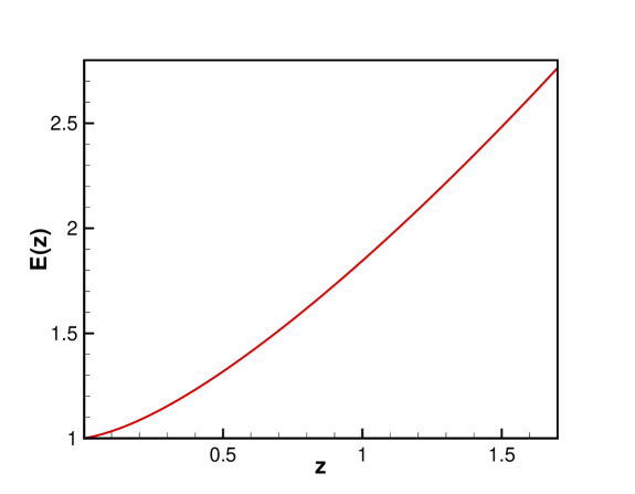
Figure 1: The dimensionless Hubble parameter, $E(z)=H(z)/H_{0}$ versus redshift derived from solving the Eq.(51) for a dark energy model with the equation of state defined in (55).

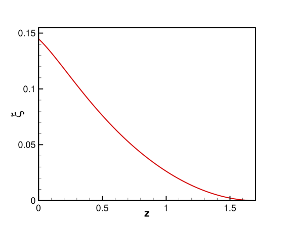
Figure 2: The deviation parameter $\xi={df}/{dR}-1$ versus redshift derived from solving the differential equation (54). Here the modified gravity is obtained from the dynamical equivalance of a dark energy with an equation of state given in (55).

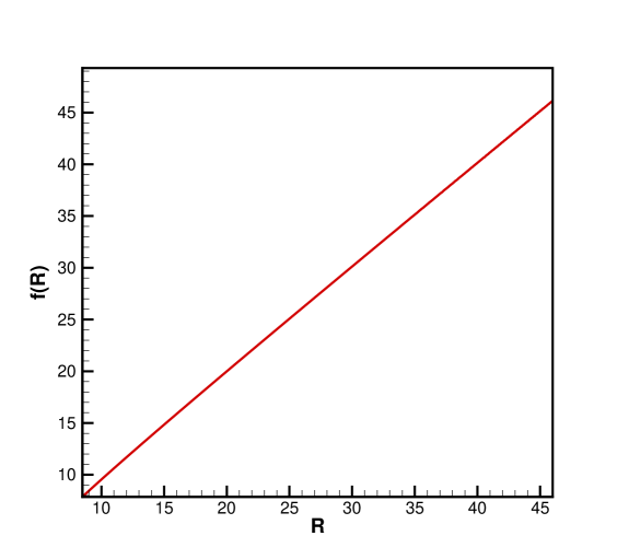
Figure 3: The modified gravity action $f(R)$, which is obtained from integration of deviation parameter $\xi$

On the other hand, for a given equation of state of a dark energy model, $\omega_{DE}(z)$, one can extract the dynamics of the universe, $E(z)$. Knowing the dynamics of the universe, from Eq.(20), the Hubble parameter is given in terms of the derivatives of the action and the Ricci scalar. The Ricci scalar in Palatini formalism is given by:

$$R=R(g)+\frac{3}{2}\frac{\nabla_{\alpha}F\nabla^{\alpha}F}{F^{2}}-\frac{3\nabla_{\alpha}\nabla^{\alpha}F}{F},$$ (52)

in which $R(g)$ is the Ricci scalar in terms of the metric and $R(g)=6\dot{H}+12H^{2}$. For the FRW metric, the Ricci scalar in the Palatini formalism is given by [45]:

$$R =-6HH^{\prime}(1+z)+12H^{2}-\frac{3}{2}H^{2}(1+z)^{2}(\frac{F^{\prime}}{F})^{2}$$ (53)

$$+ 3(1+z)^{2}HH^{\prime}\frac{F^{\prime}}{F}-6H^{2}(1+z)\frac{F^{\prime}}{F}$$

$$+ 3H^{2}(1+z)^{2}\frac{F^{\prime\prime}}{F}.$$

Now we substitute the Ricci scalar in Eq.(20) and with some algebraic manipulation we obtain a differential equation for the evolution of $F$ in terms of redshift:

$$F^{\prime\prime} - \frac{3}{2}\frac{F^{\prime 2}}{F}+F^{\prime}(\frac{H^{\prime}}{H}+\frac{2}{1+z})$$ (54)

$$- \frac{2H^{\prime}}{H(1+z)}F+\frac{\kappa}{H^{2}(1+z)^{2}}(\rho+p)=0,$$

where prime represents the derivative in terms of the redshift. Assuming $p=0$ and $\rho=\rho_{0}(1+z)^{3}$, we eliminate the density in favor of the Hubble constant, using $\kappa\rho_{0}=3H_{0}^{2}\Omega_{m}^{0}$. Finally we can solve the differential equation for a given Hubble parameter and obtain $F$ in terms of redshift.

Here we choose a smooth dark energy ansatz with the equation of state of [46]:

$$\omega=\omega_{0}+\omega_{a}\frac{z}{1+z},$$ (55)

where $\omega_{0}$ and $\omega_{a}$ are the free parameters of the model. In the case of $\omega_{0}=-1$ and $\omega_{a}=0$ we recover the $\Lambda$CDM model. Here in our simulation we choose $\omega_{0}=-1.2$, $\omega_{a}=1.5$ and use Eqs. (50) and (51) to extract the corresponding Hubble parameter for this equation of state as shown in Fig.(1). On the other hand substituting the Hubble parameter in Eq. (54) results in $F$ in terms of redshift. We set the boundary conditions in redshift of $z\sim 100$, where we anticipate to recover the general relativity condition (i.e. $F(z=100)=1$ and $F^{{}^{\prime}}(z=100)=0$). Applying the Hubble parameter in Eq.(53) we get Ricci scalar in terms of the redshift. On the other hand we substitute the Hubble parameter in (54) and get $F$ in terms of the redshift. We plot the parameter of the action deviation, $\xi\equiv F-1$ as a function of $z$ in Fig. (2). Eliminating the redshift between the $F$ and $R$ results in the derivative of the action in terms of the Ricci scalar, $F=F(R)$. One step further we do integration and find the modified gravity action $f(R)$ in terms of $R$, as shown in Fig.(3). A numerical fit to this function is:

$$f(R)\sim R-a\textrm{e}^{-\frac{R}{R_{0}}},$$ (56)

where $a\simeq 0.1$ and $R_{0}\sim 8.48H_{0}^{2}$ is the Ricci scalar at the present time. It is obvious from the form of Eq.(56) that for large scalar Ricci we will have the Einstein-Hilbert action.

It is worth to mention that for a smooth potentials of the scalar fields in the quintessence models, Bassett et al. (2002) and Corasaniti et al. (2003) [47] show that the equivalence dark energy model with this class of the quintessence models can be identify with two free parameters of $w_{0}$ and the derivation of the $w$ at the present time (i.e. $w(z)=w_{0}+\frac{w_{a}z}{1+z}$). We did our analysis based on this class of the dark energy models and didn’t test in the cases that $w(z)$ has dramatic variation with to redshift.

4.2 Reconstruction of the Action in the Modified Gravity

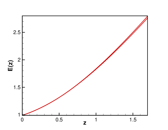
Figure 4: The reconstructed Hubble parameter with 1$\sigma$ confidence level obtained from the reconstruction of 100 ensemble of SNAP data.

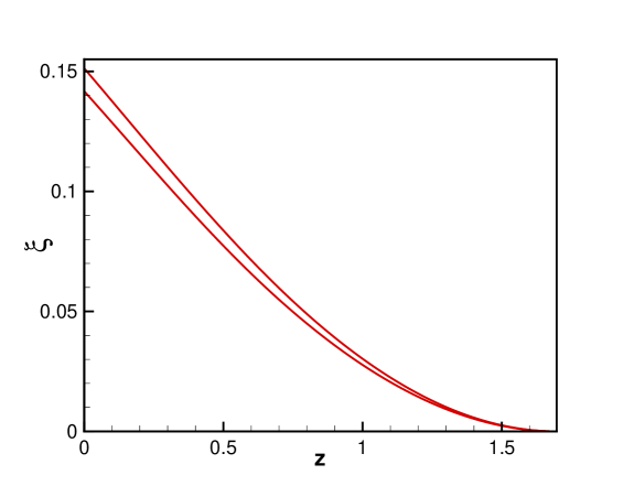
Figure 5: The reconstructed deviation parameter $\xi={df}/{dR}-1$ with 1$\sigma$ confidence level obtained from the synthetic SNAP data. The uncertainly in $\xi$ indicated with the solid lines, represents different realizations of SNIa data in an ensemble of 100 data set.

Our approach for reconstruction of the action is based on the measurement of the distance modulus of the SNIa data. From the SNIa data we can make a continues function for the distance modulus as a function of redshift (i.e. $\mu(z)$), using the smoothing method [48, 49, 50] as described in [51]. The smoothing method suffers from the low statistics of the SNIa data where it has been shown in [21] that at least $\sim 1500$ SNIa data with the quality of Union sample data set [52] is essential to generate a reliable distance modulus.

Here we repeat the same procedure with 1998 synthetic SNIa data with the quality predicted by SNAP project in the redshift range of $0.1<z<1.7$. We also add 25 SNIa data from Nearby Supernova factory project in the redshift of $z<0.1$ to have a full range coverage of SNIa data [50, 51]. Now we use the hypothetical cosmological model as described in Eq. (55) for generating the corresponding luminosity distance for the SNIa data with a systematic error of $\sigma_{sys}=0.07$ in SNAP.

After generating the synthetic distance modulus, we obtain the best curve resulting from the smoothing of the simulated data. For the smoothing discrete data, we first take an initial guess model for the distance modulus based on $\Lambda CDM$ model. Then we smooth the subtraction of the distance modulus of simulated data from the guess model using a Gaussian function as below:

$$\mu^{d}(z)=N(z)\sum_{i}[\mu^{g}(z)-\mu^{sim}(z_{i})]\exp{\frac{-(z-z_{i})^{2}}{2\Delta^{2}}},$$ (57)

where

$$N(z)^{-1}=\sum_{i}\exp[\frac{-(z-z_{i})^{2}}{2\Delta^{2}}],$$ (58)

$z_{i}$ represents the redshift of each SNIa in the simulated SNAP sample. The sum term is considered for all 2023 SNAP simulated data sample, $\mu^{sim}(z_{i})$ is the simulated distance modulus and $\mu^{g}(z)$ is a continues function generated by the guess model. $N(z)$ is a normalization factor, $\Delta$ is a suitable redshift window function and $\mu^{d}(z)$ is a smoothed continues function for the residual of luminosity distance in terms of redshift. Finally we add the smoothed distance modulus to the guess model to generate the new smooth function for the distance modulus:

$$\mu^{s}(z)=\mu^{g}(z)+\mu^{d}(z).$$ (59)

We repeat this procedure using $\mu^{s}(z)$ as the new guess model. It can be shown that after a finite time of irritations, the $\chi^{2}$ of the smoothed function with respect to observed data will converge to a fixed value[51]. Now we have a continues distance modulus function in which the Hubble parameter in terms of redshift can be obtained by:

$$H(z)=[\frac{d}{dz}(\frac{d_{L}(z)}{1+z})]^{-1}.$$ (60)

In order to calculate the uncertainty of this procedure, we generate an ensemble of the SNIa data and extract the corresponding Hubble parameters. Fig.(4) shows the reconstructed Hubble parameter with 1$\sigma$ level of confidence.

Now we can extract the modified gravity action in Palatini formalism through the method of inverse problem [53] in the Palatini formalism as discussed in the last part [21]. Applying the Hubble parameter from Eq.(60) in Eq.(54), we obtain $\xi$ in terms of redshift as plotted in Fig. (5) with 1$\sigma$ level of confidence. Numerical integration of $F(R)$ provides the action, $f(R)$.

4.3 Reconstruction of structure formation indicators and matter density Power Spectrum

In this section by applying the reconstructed action, we obtain the density contrast and corresponding power spectrum of the matter and compare it with that from the dark energy model. We start the procedure by reconstructing the screened mass function by substituting the numerical value for the first derivative of the action in Eq.(26). The corresponding screened mass function for this action is plotted in Fig.(6). At redshifts above $z\gtrsim 1.5$, the screened mass function approaches to unity in which the GR structure formation is recovered. It should be noted that the screened mass function does not depend only on the chosen MG action but also it depends on the wavenumber of the structures. One step further to indicate the probable different predictions of metric and Palatini formalism in matter density power spectrum we also plot the screened mass function in metric formalism $Q^{met}(k,z)$ in Fig.(7) by applying the reconstructed dynamics of universe and MG action in Eq.(46).

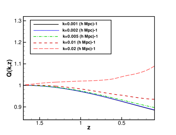
Figure 6: Screened mass function in Palatini formalism in terms of the redshift and wavenumbers of the structures for the action equivalent to the dark energy with the equation of state in Eq. (55).

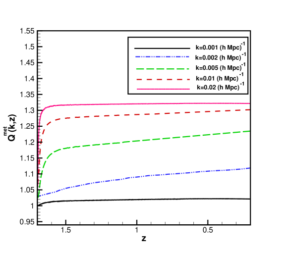
Figure 7: Screened mass function in metric formalism in terms of redshift and wavenumbers of the structures for the action equivalent to the dark energy with the equation of state in Eq. (55).

The comparison of two Figures (6) and (7) shows the different scale dependence of screened mass function in both formalisms and consequently the different effects on the modification to the Poisson equations. A crucial point to indicate is that this difference arise from the structure formation effects. This is because the background dynamics $H=H(z)$, is the same for two formalisms obtained independently from SNIa data. The difference comes from the definition of Ricci scalar $R(g)=6\dot{H}+12H^{2}$ and modified Friedmann Eq.(47) in metric formalism and also the screened mass function defined in Eq.(46).

In Palatini formalism, in small wavenumbers, correspond to the larger structures, $Q(k,z)$ descends for the later times, means weakening of the gravitational strength in the Poisson equation. On the other hand, in the smaller structures $Q$ is larger than one (see. Fig.6) which makes a faster growth of the structures compared to the GR. The dependence of $Q$ to the wavenumber is similar to the dispersion relation in optics in which different length structures’ gravitational response is different [54]. The deviation of $Q$ from unity and also its dependence on $k$ affects the growth of the density contrast and subsequently the power spectrum of the structures. In Palatini formalism the deviation from $Q=1$ is large at the larger scales, in contrast in metric formalism we always have a faster growth in structures and the the deviation is larger in small scales. These differences can put their fingerprint in LSS observations. In what follows we will solve the differential equation governing the density contrast for various wavenumbers and finally obtain the corresponding power spectrum of the structures.

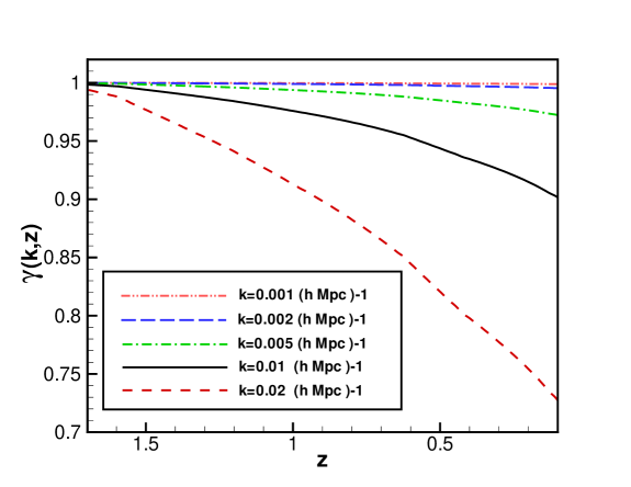
Figure 8: The gravitational slip parameter is plotted versus redshift for different wavenumbers of the structures.

In order to solve Eq.(3.2) we need to obtain the gravitational slip parameter. Substituting the action in Eq.(33), we reconstruct the gravitational slip parameter as shown in Fig.(8). The gravitational slip parameter is equal to one for higher redshifts and GR is recovered. For the later times at lower redshifts $\gamma$ deviates from GR. This deviation is larger for the small structures. The variation of $Q$ and $\gamma$ with respect to GR indicates that the power spectrum of the structures should deviate in comparison with the DE models. It is worth to mention that the cosmic shear statistics as well as ISW effect is sensitive to the gravitational slip parameter and provides a promising tool for distinguishing between the models.

For calculating the evolution of the density contrast we reexpress Eq.(3.2) in terms of redshift as below:

$$\delta_{k}^{{}^{\prime\prime}}+A(k,z)\delta_{k}^{{}^{\prime}}+B(k,z)\delta_{k}=0,$$ (61)

where the coefficients A and B are defined as:

$$A =\frac{E^{{}^{\prime}}}{E}+\frac{1}{1+z}-\alpha(\tilde{k},z)(\frac{2}{1+z}-\frac{9(1+z)\Omega^{0}_{m}}{\tilde{k}^{2}}Q^{{}^{\prime}}),$$

$$B =\alpha(\tilde{k},z)[-\frac{3}{2}\gamma^{-1}\Omega^{0}_{m}\frac{Q(1+z)}{E^{2}}-\frac{9\Omega^{0}_{m}}{2\tilde{k}^{2}}(\frac{Q}{1+z}-Q\frac{E^{{}^{\prime}}}{E}$$

$$- (1+z)Q^{{}^{\prime}}\frac{E^{{}^{\prime}}}{E}-Q^{{}^{\prime}}-(1+z)Q^{{}^{\prime\prime}})],$$ (63)

and $\alpha(\tilde{k},z)\equiv{2\tilde{k}^{2}}/[{2\tilde{k}^{2}+9\Omega_{m}^{0}Q(1+z)}]$, where ${\tilde{k}\equiv{k}/{H_{0}}}$. For the case that $Q^{{}^{\prime}}=Q^{{}^{\prime\prime}}\sim 0$ and $\tilde{k}\gg 9\Omega_{m}^{0}Q(1+z)$ we will recover the general form of density contrast evolution as:

$$\delta^{{}^{\prime\prime}}+\left[\frac{E^{{}^{\prime}}}{E}-\frac{1}{1+z}\right]\delta^{{}^{\prime}}-\frac{3}{2}\frac{\Omega^{0}_{m}(1+z)}{E^{2}}\gamma^{-1}Q\delta=0.$$ (64)

In this work within the Palatini formalism we solve the general form of Eq.(61). The result for the reconstructed modified gravity is plotted in Fig.(9) for the various wave numbers. Here we take the initial condition of the density contrast from the Harrison-Zeldovich spectrum before the turn over point of the power spectrum around $k\simeq 0.02$.

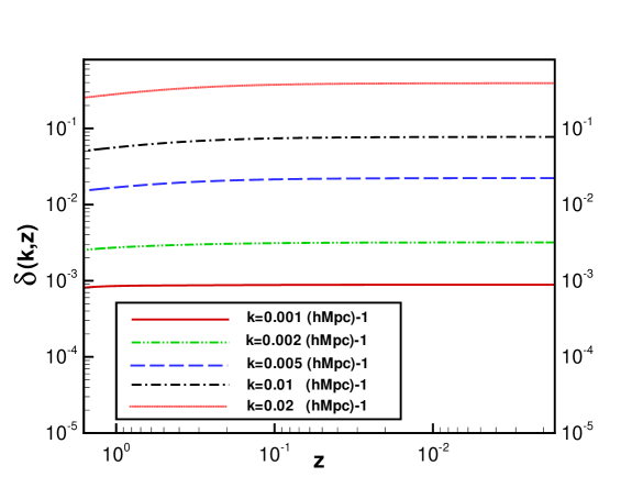
Figure 9: The matter density contrast in Palatini formalism is plotted versus redshift for different wavenumbers.

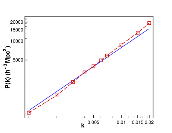
Figure 10: The power spectrum of MG theory in terms of wavenumber(dashed line) is plotted in comparison to Harrison-Zeldovic power spectrum (solid line). For the MG model the slop of the power spectrum is $n_{f}=1.21^{+0.13}_{-0.19}$.

By solving Eq.(61) we obtain the power spectrum of the structures at the present time as plotted it in Fig. (10) where the slope is $n_{f}=1.21^{+0.13}_{-0.19}$. It should be noted that at these large scales (i.e. $k<0.01$) we don’t have accurate data from the large scale structure observations [55]. In order to compare the two models with nowadays LSS survey data, we should study the nonlinear regime of power spectrum which is not in the scope of this work. We note that the transformation of the linear power spectrum to nonlinear regime by analytical methods is strictly model dependent and it is not yet well understood [56].

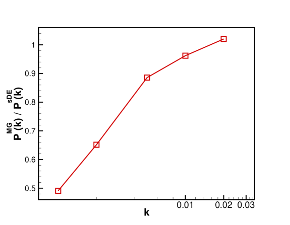
Figure 11: The fraction of MG to sDE power spectrum is plotted versus wavenumbers at the present epoch.

In order to compare power spectrum predicted from the equivalence DE and MG models, we obtain the density contrast in DE model for various wavenumbers at the present time. We note that the only difference in the differential equation governing the density contrast evolution of the MG and DE is that, for the case of DE we let $Q,\gamma=1$. We plot the fraction of the power spectrum of the matter density in the MG to that in the equivalence DE in terms of wavenumber at present time in Fig.(11). While we have equivalent dynamics for the background expansion of the universe, the power spectrum from the MG and DE models are different. For the structures with the size of $k<0.01$ the MG power spectrum is smaller than the DE model, as the screened mass in these scales is less than unity. On the other hand for structures with the scale of $k>0.01$ the screened mass is larger than unity and the ratio of the two power spectrums increases. The dependence of the power spectrum to the wavenumber can provide an observational tool to distinguish between these two models. Qualitatively we can also assert that as the screened mass function in small scales is bigger than unity, we will have an enhancement in mater density power spectrum in comparison to the equivalent sDE model.

Another observational parameter in the structure formation is the dynamics of the growth index factor defined as $f={d\ln\delta}/{d\ln a}$ in terms of the redshift. We rewrite the differential Eq.( 61) in terms of growth index factor $f$ as below:

$$f^{{}^{\prime}}-\frac{f^{2}}{1+z}+(A-\frac{1}{1+z})f-B(1+z)=0,$$ (65)

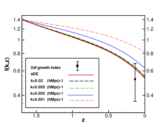
Figure 12: The growth index function is plotted versus redshift for various wavenumbers. The observational data from the 2dF survey is represented with the corresponding error bar.

where A and B are defined from Eqs. (4.3) and (63). We plot the growth index in the MG and sDE in Fig.(12) with the observational data from the 2dF survey [57]. For the higher redshifts the growth index for the two models is the same while for the later times they diverge. An observational way to distinguish the MG from the DE model is measuring the growth index for various wavenumbers. For the case of DE model, the growth index is independent of the size of structure, as the structure formation equation for the scales larger than the Jeans length is independent of the $k$ while in the MG model, screened mass relates the growth index of the structure to its size. Future surveys of the large scale structure may reveal the growth index in terms of wavenumber of the structures.

5 ISW as probe to distinguish between DE and MG models

In this section we examine the effect of MG on Integrated Sachs-Wolfe effect (ISW) [58] and compare it with the dynamically equivalent dark energy model. ISW effect is one of the important cosmological probes which traces the effect of dynamics of the potentials on the photons of the cosmic microwave background radiation (CMB). The effect of MG on ISW effect has already been studied in several works in metric formalism as in [59]. This effect has been also studied in a class of $f(R)$-gravities in Palatini formalism where the deviation from $\Lambda$CDM of this models occurs at a higher redshift (known as the early time f(R) gravities)[61] and the results are compared with ordinary $f(R)$ gravities. It was shown that the matter power spectrum is more sensitive to gravity modification than the ISW-effect, which is compatible to our results obtained in this section, although their specific choice of gravity action caused to a deviation in ISW effect in higher l-moments [60].

We start with the reconstruction of the perturbed potential $\Phi$ which is a relevant parameter in the ISW and weak lensing observations. Using the Poisson equation of (24) for MG, $\Phi$ is given in terms of the density contrast and screened mass function as follows:

$$\Phi(k,z)=\frac{3\Omega_{m}^{0}(1+z)}{2{\tilde{k}}^{2}}\delta_{m}Q(k,z).$$ (66)

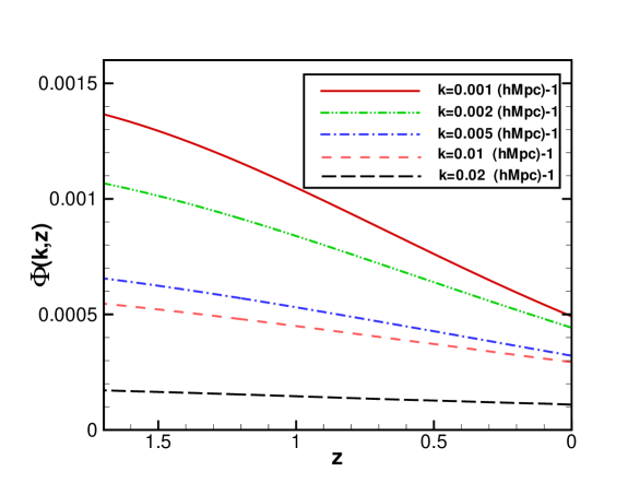
Figure 13: The perturbed potential $\Phi$ in MG theory in terms of redshift for various wavenumbers.

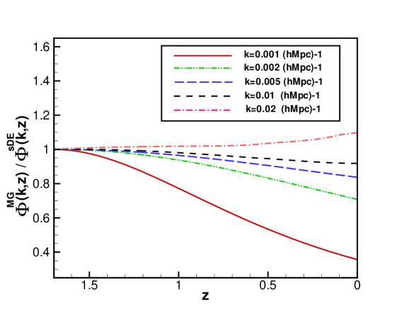
Figure 14: The fraction of perturbed potential in MG to that in the sDE model in terms of redshift for various wavenumbers.

Substituting the numerical values of matter density contrast and the screened mass function, we obtain the potential in terms of redshift for various wavenumbers. The result is plotted in Fig.(13). For comparison with the dark energy model, we express the relative magnitude of Potential in MG and sDE models as below:

$$\frac{\Phi^{MG}(k,z)}{\Phi^{sDE}(k,z)}=\frac{\delta^{MG}_{m}}{\delta^{sDE}_{m}}Q(k,z).$$ (67)

Fig.(14) shows this ratio in terms of redshift for various wavenumbers. Eq.(67) shows that this ratio is proportional to the relative magnitude of density contrast and screened mass function. In the zeroth order the density contrast growth is approximately equal to density contrast in sDE. The relative magnitude of potentials diverge from unity in large scales as the screened mass function k-dependance. Although the k-dependence of $\gamma$-parameter has a secondary effect on the growth of density contrast through Eq.(61).

Now we apply results from the dynamical evolution of potential in the ISW effect. ISW effect is caused by the time variation in the cosmic gravitational potential, as the CMB photons pass through the structures. In this effect the amount of the energy gain of the photons due to the gravitational potential of the structure may not be equal to the energy lose of the photons when they leave the potential well. The result of this effect is an extra anisotropy on the CMB map.

In generic case, the CMB anisotropy due to the ISW is given by

$$\Theta_{l}(k,\eta_{0})=\int_{0}^{\eta}d\eta e^{-\tau}\left[\dot{\Psi}(k,\eta)-\dot{\Phi}(k,\eta)\right]j_{l}(k(\eta_{0}-\eta)),$$ (68)

where $\Theta_{l}$ represents the l-th moment of temperature contrast defined in Eq.(5), $\tau$ is the optical depth of the photons which we can neglect it in ISW calculations, $j_{l}$ is the Bessel function and $\eta$ is the conformal time and ”.” in this equation represents derivative with respect to the conformal time. Since in the smooth dark energy models $\Phi=-\Psi$ Eq. (68) reduces to:

$$\Theta_{l}^{sDE}(k,\eta_{0})=\int_{0}^{\eta}d\eta\left[-2\dot{\Phi}^{DE}(k,\eta)\right]j_{l}(k(\eta_{0}-\eta)),$$ (69)

superscript ”$sDE$” on $\Theta$ indicates ISW effect in sDE model. For calculating the ISW in the equivalent dark energy model, we use the numerical value for the $\Phi$ which is obtained in the last section. On the other hand, since in the MG, the two potentials of $\Phi$ and $\Psi$ are not equal and relates by the slip parameter in Eq. (33), we eliminate $\Psi$ in favor of $\Phi$ in Eq.(68) and rewrite the ISW effect in the MG models as follows:

$$\Theta_{l}^{MG}(k,z)=\int_{z\sim 1100}^{z=0}dz\frac{d}{dz}\left[-\Phi^{MG}(\gamma^{-1}+1)\right]j_{l}[\tilde{k}\int_{0}^{z}\frac{dz^{{}^{\prime}}}{E(z)^{{}^{\prime}}}],$$ (70)

where the superscript of ”$MG$” in $\Theta_{l}$ indicates the temperature anisotropy in the MG model. For simplicity in the numerical calculation, we reexpress time derivatives in terms of redshift and since $\Phi$ is almost a constant function beyond the redshift of $z\simeq 1.7$ (see Fig. 13), we put a cutoff in the numerical integration up to this redshift.

In order to express our results in terms of observable parameter, we obtain the $\Theta_{l}$ in terms of CMB power spectrum, $C_{l}$. The variance of temperature fluctuations, $\delta_{ll^{{}^{\prime}}}\delta_{mm^{{}^{\prime}}}C_{l}=<a_{lm}a^{*}_{l^{{}^{\prime}}m^{{}^{\prime}}}>$ can be related to $\Theta_{l}$ as below [29]:

$$C^{ISW}_{l}=\frac{2}{\pi}\int_{0}^{\infty}dkk^{2}P(k)|\frac{\Theta_{l}(k)}{\delta(k)}|^{2}.$$ (71)

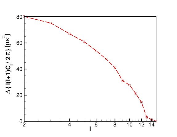
Figure 15: The difference of $\Delta C_{l}=C^{sDE}_{l}-C^{MG}_{l}$ between the equivalent DE and MG models in terms of $l$.

We note that for the small scale structures, the time derivative of the potential in Fig. (13) is almost zero. Hence we expect that in the ISW, small structures ( large $l$s ) will not be modified. So we examine only small moments for calculating deviation from the standard CMB power spectrum. Taking small $l$s in the range of $l<10$ we calculate $C_{l}$s both in the MG and the equivalent DE model. The numerical difference of the power spectrum $\Delta C_{l}=C^{sDE}_{l}-C^{MG}_{l}$ between the DE and MG models in terms of $l$ is shown in Fig.(15). Here for the small $l$s we have more contrast than the large $l$s.

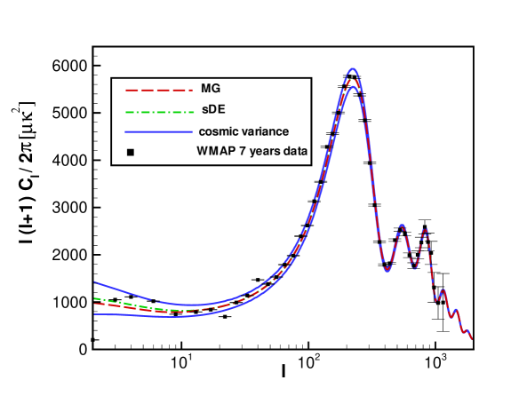
Figure 16: Power Spectrum of CMB for Modified gravity and equivalent dark energy model in the Palatini formalism.

Finally we express our analysis in CMB power spectrum for the MG and sDE models and compare them with the observational data. We use the CMB-fast code to plot the power spectrum for the equation of state defined in Eq.(55). As we showed in Fig. (15), the difference in the power spectrum between the two equivalent DE and MG models is in the small $l$s and for the larger $l$s the power spectrum of the two models coincide to each other. For smaller $l$s, we use the numerical results of Fig. (15) to obtain the power spectrum of the MG from the DE model. Fig.(16) compares the power spectrum from the MG and DE model with the latest WMAP-7 years data [62]. We note that this deviation is smaller than the cosmic variance in the WMAP data.

6 Conclusion

One of the important questions in the problem of the acceleration of the universe is either this acceleration is produced by a dark energy fluid or that is a manifestation of the gravity modification. It has been shown that the expansion history of the universe can not dynamically distinguish between these two models and at this stage they are equivalent.

In this work we compared various aspects of the structure formation in the Modified Gravity (MG) and smooth Dark Energy (sDE) models. We used an ansatz for the equation of state of a dark energy model and obtained the equivalent modified gravity . Using a synthetic SNIa data set from the SNAP observation, we did the inverse problem approach and obtained the effective action of the gravity (i.e. $f(R)$). It has been shown that the structure formation unlike to the background dynamics can distinguish between these two models.

In the modified gravity, the modification of the Einstein-Boltzman equation for the structure formation has extra terms compare to the sDE model. This modification can be given in terms of screened mass function and gravitational slip parameter. We obtained these two parameters in the MG model and solved the differential equation for the evolution of the structure formation. Using the Harrison-Zeldovich initial condition for the structures, finally we obtained the power spectrum and the growth index of the structures in the two scenarios in the linear regime of the structure formation. We have shown that for the structures with the larger size, the effective spectral index at the present time is slightly more than one. From the observational point of view, sampling of large scale structure more than $100$Mpc is needed to test this effect. On the other hand, we showed that the growth index parameter in the MG unlike to the sDE models is a scale dependent parameter. Next generation of peculiar velocity survey may measure this effect. Finally we obtained the effect of the MG structure formation on the Integrated Sachs-Wolfe effect on CMB map. We showed that the deviation of the CMB power spectrum due to the MG is larger in the small $l$s, however it is not too large to distinguish between the two models due to the uncertainty from the cosmic variance.

Appendix A Structure formation probes in metric formalism

Here in this appendix, we obtain the evolution of matter density contrast in the metric formalism and consequently derive the matter power spectrum and growth index in order to compare them with that in the Palatini formalism.

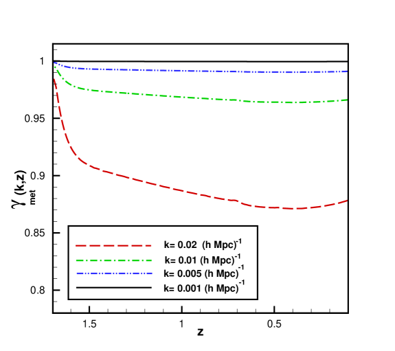
[h]

Figure 17: The gravitational slip parameter in metric formalism for different wavenumbers. The Long dashed line correspond to small scales $k=0.02$, where we have the most deviation in this parameter from GR value.

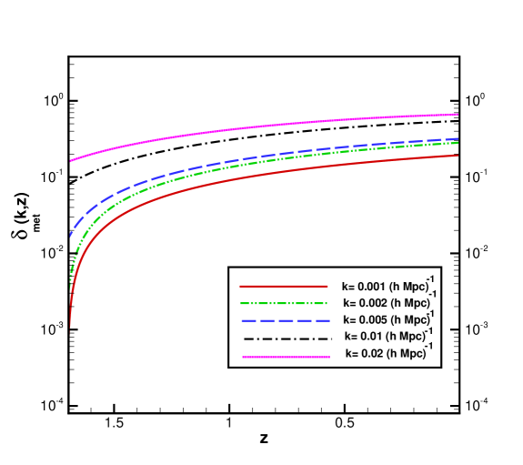
Figure 18: The density contrast of the mater in metric formalism in terms of redshift and wavenumber is plotted. parameter in metric formalism for different wavenumbers.

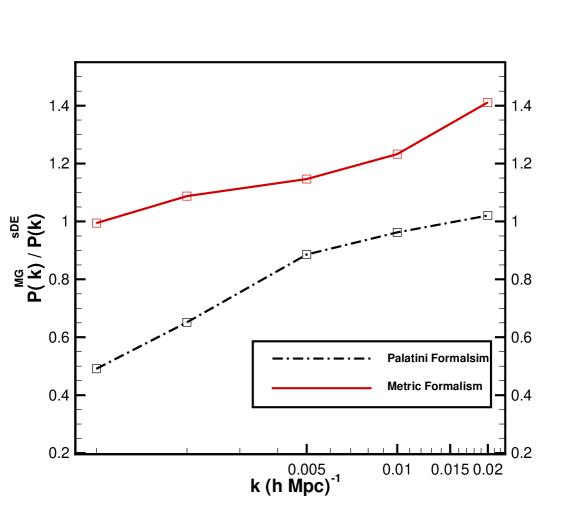
Figure 19: The relative power Spectrum of Modified gravity and smooth Dark Energy is plotted versus wavenumber for Metric formalism(solid line), Palatini Formalism (dash-dot line)

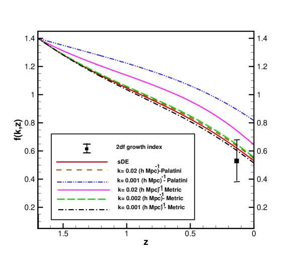
Figure 20: The growth index factor is plotted versus redshift for different wavenumbers in Metric formalism (dotted, long dash, dash-dot lines), Palatini Formalism (dashed and dash-dot-dot lines) and sDE models(solid line)

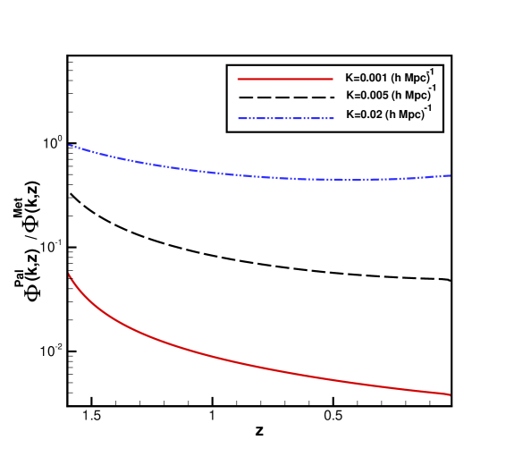
Figure 21: The relative magnitude of gravitational potential in Metric and Palatini formalism plotted versus redshift for different wavenumbers

In order to determine the matter density evolution we use Eq.(45), where we can rewrite it, in terms of redshift as below:

$$\delta^{{}^{\prime\prime}}+\left[\frac{E^{{}^{\prime}}}{E}-\frac{1}{1+z}\right]\delta^{{}^{\prime}}-\frac{3}{2}\frac{\Omega^{0}_{m}(1+z)}{E^{2}}\gamma_{met}^{-1}Q_{met}\delta=0.$$ (72)

The above equation has the same form as in the Palatini formalism, Eq.(64), however the difference is in the value of the screened mass function and the gravitation slip parameter in the two modified gravity formalism.

The screened mass function is obtained in Sec.(4) and plotted in Fig.(7). For calculating the gravitational slip parameter, due to the slow change of the action over the Hubble time we neglect the term of $\delta\Box F(R)$ in the perturbation of the trace of the field equation (41). We follow the same procedure an in the Palatini formalism and obtain the gravitational slip parameter in terms of reconstructed $F$ from Eq.(48) and the screened mass $Q_{met}$ from Eq.(46) which results in

$$\gamma_{met}=\left[1-\frac{2m(1+z)^{2}{\tilde{k}}^{2}}{\tilde{R}FQ_{met}(m-1)}\right]^{-1}.$$ (73)

The gravitational slip parameter in the metric formalism is Plotted in Fig.(17) for different wavenumbers. Similar to the Palatini case, Fig.(8), the gravitational slip parameter deviates from its GR value $\gamma=1$ in small scales. Knowing the screened mass function and gravitational slip parameter, we solve the differential Eq.(72) governing the evolution of density contrast. The results is plotted in Fig.(18).

In the next step we compare the relative magnitude of power spectrum of metric-MG to sDE, $P_{Met}/P_{sDE}$ and Palatini-MG to sDE , $P_{Pal}/P_{sDE}$ both plotted in Fig.(19). As we except because the variation of screened mass function from GR value $Q>1$ in small scales, we get a amplification in power spectrum in large $k$’s, which shows a different prediction than the Palatini formalism in which there is a suppression in large scales.

Using Eq.(72) we can also reexpress the growth index function $f\equiv\frac{d\ln\delta}{d\ln a}$ in terms of redshift as:

$$f^{{}^{\prime}}-\frac{f^{2}}{1+z}+\left[\frac{E^{{}^{\prime}}}{E}-\frac{2}{1+z}\right]f+\frac{3}{2}\frac{\Omega_{m}^{0}}{E^{2}}\gamma^{-1}_{met}Q_{met}(1+z)^{2}=0$$ (74)

For comparison with the Palatini formalism, we plot the growth index for large and small scales in both metric and Palatini formalism in Fig.(21).

Finally the last comparison is done for the relative magnitude of gravitational potential $\Phi$ in both formalism. From Poison equation, it is straightforward to calculate this ratio as:

$$\frac{\Phi_{Pal}}{\Phi_{Met}}(k,z)=\frac{\delta^{Pal}_{m}Q_{Pal}}{\delta^{Met}_{m}Q_{Met}}$$ (75)

The results for three wavenumbers is plotted in Fig.(21). The relative magnitude of gravitational potential in higher-redshifts converge to unity for all wavenumbers. This is because the screened mass functions, in both formalism converge to unity and the evolution of matter density contrast in deep matter dominated era is proportional to the scale factor.

References

- [1] A.G. Riess et al., Astron. J. 116, 1009 (1998); S. Perlmutter et al., Astrophys. J. 517, 567 (1999); A.G. Riess et al., Astrophys. J. 607, 665 (2004); M. Hicken et al., Astrophys. J. 700, 1097 (2009).
- [2] J. Dunkley et al., Astrophys. J. Suppl. 180, 306 (2009).
- [3] S.M. Carroll et al. Annual Review of Astron. Astrophys. 30, 499 (2001); T. Padmanabhan Phys. Rept. 380, 235 (2003).
- [4] T.M. Davis et al., Astrophys. J. 666, 716, (2007).
- [5] S. Weinberg, Rev. Mod. Phys. 61, 1, (1989).
- [6] P.J.E. Peebles and B. Ratra, Rev. Mod. Phys. 75, 559 (2003); S. Rahvar and M.S. Movahed, Phys. Rev. D 75, 023512 (2007).
- [7] Copeland et al., Int. J. Mod. Phys. D 15 1753 (2006); S.M. Carroll, V. Duvvuri, M. Trodden, M.S. Turner, Phys. Rev D 70, 043528 (2004); T.P. Sotiriou and Valerio Faraoni, arXiv:0805.1726; S. Nojiri, S.D. Odintsov, Phys. Rev. D 68, 123512 (2003);S. Nojiri and S.D. Odintsov, Gen. Rel. Grav. 36, 1765 (2004) S. Baghram, M. Farhang and S. Rahvar, Phys. Rev. D 75, 044024(2007).
- [8] R. Saffari and S. Rahvar, Phys. Rev. D 77, 104028 (2008).
- [9] B. Jain, P. Zhang, Phys. Rev. D 78, 063503 (2008); M. S. Movahed, S. Baghram, S. Rahvar, Phys. Rev. D 76, 044008 (2007); S. Baghram, M.S. Movahed, S. Rahvar, Phys. Rev. D 80, 064003 (2009).
- [10] V. Faraoni, Phys. Rev. D 75, 029902(E) (2007).
- [11] Sh. Tsujikawa, Living Rev. Rel. 13, 3 (2010).
- [12] V. Flanagan Phys. Rev. Lett. 92 071101 (2004); V. Flanagan Class. Quant. Grav. 21 3817 (2004); Iglesias, A., N. Kaloper, A. Padilla, and M. Park, 2007, Phys. Rev. D 76, 104001.
- [13] E. Barausse et al., Class. Quant. Grav. 25, 062001 (2008).
- [14] T. Kobayashi and K.I. Maeda, Phys. Rev. D 78 064019 (2008); E. Barausse et al., Class. Quant. Grav. 25, 105008 (2008).
- [15] A. Upadhye and W. Hu, Phys. Rev. D 80, 064002 (2009); T. Kobayashi and K.I. Maeda, Phys. Rev. D 79 024009 (2009); G.J. Olmo, Phys. Rev. D 78, 104026 (2008); S. Appleby and R. Battye, Phys. Lett. B 654, 7 (2007); A.A. Starobinsky, JETP lett. 86, 157 (2007).
- [16] W. Hu and I. Sawicki, Phys. Rev. D 76, 064004 (2007);
- [17] A.A. Starobinsky, JETP lett. 86, 157 (2007).
- [18] E. E. Flanagan, Phys. Rev. Lett. 92, 071101 (2004); E.E. Flanagan Class. Quant. Grav. 21, 3817 (2004); Iglesias et al. Phys. Rev. D 76, 104001 (2007), A.D. Dolgov and M. Kawasaki, Phys. Lett. B, 573, 1 (2003).
- [19] B. Li, D.F. Mota and D.J. Shaw, Phys. Rev. D 78, 064018 (2008); B. Li, D.F. Mota and D.J. Shaw, Class. Quant. Grav. 26, 055018 (2009).
- [20] E. Bertschinger and P. Zukin, Phys. Rev. D 78, 024015 (2008).
- [21] S. Baghram and S. Rahvar,Phys. Rev. D 80, 124049 (2009).
- [22] L. Pogosian and A. Silvestri, Phys. Rev. D, 77, 023503 (2008).
- [23] A. Lue, R. Scoccimarro, G. Starkman , Phys. Rev. D 69, 044005 (2004); S.F. Daniel, R.R. Caldwell, A. Cooray, A. Melchiorri, Phys. Rev. D 77, 103513 (2008); R. Bean, arXiv:0909.3853.
- [24] H. Wei and S.N. Zhang, Phys. Rev. D 78, 023011 (2008).
- [25] M. Kunz, D. Sapone, Phys. Rev. Lett. 98, 121301 (2007); T. Koivisto and D.F. Mota, J. Cosmol. Astropart. Phys. 018, 0806 (2008).
- [26] P. Zhang et al., arXiv:0809.2836.
- [27] R. Reyes et al., Nature 464, 256 (2010)
- [28] V.F. Mukhanov, H.A. Feldman, &R.H. Brandenberger, Phys. Rep., 215, 203 (1992).
- [29] Dodelson, Modern Cosmology, Cambridge University Press, (2002).
- [30] C.P. Ma and E. Bertshinger, Astrophys. J. 455, 7 (1995).
- [31] J.M. Barddeen, Phys. Rev. D 22, 1882 (1980).
- [32] L.Amendola et al.,J.Cos.Astro.part. ,0804, 013 (2008); G.B. Zhao, L. Pogosian, A. Silvestri, J. Zylberberg, Phys. Rev D 79, 083513 (2009); F.Schmidt,Phys. Rev. D 78 , 043002 (2008); B.Jain and P. Zhang, Phys. Rev. D 78,063503(2008).
- [33] T. Padmanabhan, Structure Formation in the Universe (Cambridge University Press, Cambridge, England, 1993); R.H. Brandenberger,In The Early Universe and Observational Cosmology, edited by N. Breton, J.L. Cervantes-Cota, and M. Salgado, Lecture Notes in Physics Vol. 646(Springer, Berlin/Heidelberg, 2004),p. 127; K. Koyama and R. Maartens, J. Cosmol. Astropart. Phys. 01 (2006) 016.
- [34] B. Boisseau et. al, Phys. Revv. Lett. 85, 2236 (2000).
- [35] W. Hu,Astrophys. J. 506, 485 (1998).
- [36] C. Schimd et al., Astron. Astrophys. 463, 405 (2007); I. Brevik, S. Nojiri, S.D. Odintsov, L. Vanzo, Phys. Rev. D 70, 043520 (2004); S. Nojiri and S.D. Odintsov, Phys. Rev. D 72, 023003 (2005).
- [37] M. Malquarti and A.R. Liddle, Phys. Rev. D, 66, 123506 (2002).
- [38] T.P. Sotiriou, Phys. Rev. D 79 044035 (2009); G.J. Olmo, and P. Singh, J. Cosmol. Astropart. Phys. 0901, 030 (2009); A. Ashtekar, Gen. Rel. Grav. 41, 707 (2009).
- [39] G. Allemandi, A. Borowiec, M. Francaviglia, Phys. Rev. D 70, 043524(2004); M. Amarzguioui et al., Astron. Astrophys. 454, 707 (2006); T.P. Sotiriou and S. Liberati, Ann. Phys. (N.Y.) 322, 935 (2007).
- [40] Sh. Tsujikawa, K. Uddin, R. Tavakol, Phys. Rev. D 77, 043007 (2008).
- [41] T. Koivisto and H.K. Suonio, Class. Quant. Grav. 23, 2355 (2006).
- [42] Y.S. Song et al., arXiv:1001.0969.
- [43] L. Amendola and Sh. Tsujikawa, Dark Energy, Theory and Obsrevation, Cambridge 2010.
- [44] T. Koivisto, Phys. Rev. D, 73, 083517 (2006).
- [45] T. P. Sotiriou and Valerio Faraoni, Review commissioned by Rev. Mod. Phys. (2008)
- [46] M. Chevallier and D. Polarski, Int. J. Mod. Phys. D 10, 213 (2001); E.V. Linder, Phys. Rev. Lett. 90, 091301 (2003).
- [47] B. A. Bassett, M. Kunz, J. Silk, and C. Ungarelli, Mon. Not. Roy. Astron. Soc. 336, 1217 (2002); P. S. Corasaniti and E. J. Copeland, Phys. Rev. D 67 063521 (2003).
- [48] S. Capozziello, V.F. Cardone, A. Troisi, Phys. Rev. D 71, 043503 (2005).
- [49] A.A. Starobinsky, JETP Lett. 68, 757 (1998); D. Huterer and M.S. Turner, Phys. Rev. D 60, 081301 (1999); T.D. Saini, S. Raychaudhury, V. Sahni, A.A. Starobinsky, Phys. Rev. Lett. 85, 1162 (2000).
- [50] G. Aldering et al., arXiv:astro-ph/0405232.
- [51] A. Shafieloo et al., Mon. Not. Roy. Astron. Soc. 366, 1081 (2006).
- [52] M.Kowalski et al. Astrophys. J. 686, 749 (2008).
- [53] S. Rahvar and Y. Sobouti, Mod. Phys. Lett. A 23, 1929 (2008).
- [54] S. Tsujikawa, R. Gannouji, B. Moraes, D. Polarski, Phys. Rev. D, 80, 084044 (2009).
- [55] M. Tegmark et al., Mon. Not. Roy. Astron. Soc. 335, 887 (2002).
- [56] R.E. Smith et al., Mon. Not. Roy. Astron. Soc. 341, 11311 (2003); J.A. Peacock, Cosmological Physics (Cambridge University Press, Cambridge, England, 1999).
- [57] E. Hawkins et al., Mon. Not. Roy. Astron. Soc 346, 78 (2002).
- [58] R.K. Sachs and A.M. Wolfe, Astrophys. J. 147, 73 (1967).
- [59] Y.S. Song, H. Peiris, W. Hu, Phys. Rev. D 76, 063517 (2007).
- [60] B. Li and M.C. Chu, Phys. Rev. D,74, 104010 (2006).
- [61] P. Zhang, Phys. Rev. D 73, 123504 (2006).
- [62] N.Jarosik et al., arXiv:1001.4744.