The Mesoscopic Kondo Box: A Mean-Field Approach

Abstract

We study the mesoscopic Kondo box, consisting of a quantum spin $1/2$ interacting with a chaotic electronic bath as can be realized by a magnetic impurity coupled to electrons on a quantum dot, using a mean-field approach for the Kondo interaction. Its numerical efficiency allows us to analyze the Kondo temperature, the local magnetic susceptibility, and the conductance statistics for a large number of samples with energy levels obtained by random matrix theory. We see pronounced parity effects in the average values and in the probability distributions, depending on an even and odd electronic occupation of the quantum dot, respectively. These parity effects are directly accessible in experiments.

I Introduction

Many-body effects have been a key interest in condensed matter physics for many decades. A prime example is the Kondo effect hewson that, in its original context, refers to an increase of the resistance with decreasing temperature below the characteristic Kondo temperature $T_{K}$ in metals containing magnetic impurities. The significant progress in the fabrication of mesoscopic and nanoscopic systems has lead to many alternative realizations of Kondo systems. goldhaber98 ; cronenwett98 ; nygard00 ; Delattre A nice example is the so-called Kondo box, thimm99 where a finite number of electrons, confined in a quantum dot, is coupled to a single magnetic impurity. Their discrete energy spectrum introduces the mean level spacing $\Delta$ as new energy scale. It has been shown that physical quantities strongly deviate from the metallic behavior for $\Delta\gtrsim T_{K}$, i.e., when the size of the Kondo cloud screening the impurity would become larger than the size of the system. SimonAffleck1 ; SimonAffleck2 ; thimm99 ; italians ; balseiro For example, they show parity effects, i.e., characteristic differences for an even and odd number of electrons in the system. nakamura99 ; park03 ; montambaux98 Kondo physics in the presence of a chaotic dot geometry and disorder, respectively, has been studied within the Kondo disorder model (KDM) miranda ; mucciolo ; cornaglia06 using Anderson’s poor man’s scaling approach poorman to calculate the Kondo temperature. However, poor man’s scaling cannot describe the strong coupling phase below $T_{K}$, and non-perturbative methods are needed, for example quantum Monte Carlo simulations (QMC), QMC numerical renormalization group NRG ; NRG2 or the non-crossing approximation. NCA These methods are either numerically expensive or not reliable for low temperatures $T\ll T_{K}$. bickers The QMC has been used by Kaul et al. baranger to calculate the local magnetic susceptibility $\chi_{0}$ for three different realizations of a chaotic system showing that mesoscopic fluctuations lead to significant deviations from bulk universality. However, parity effects and systematic studies of mesoscopic fluctuations were neither considered here nor in the KDM studies.

In the present Letter we use a mean-field approach which had been developed initially for the single impurity Kondo model in a macroscopic metal, yoshimori70 and later adapted to some particular mesoscopic Kondo systems. SimonAffleck2 ; Aguado We first introduce the method in the framework of the chaotic Kondo box model. We then discuss the resulting probability distributions of $T_{K}$, $\chi_{0}$, and the conductance $G$. Their knowledge and the characteristic differences between even and odd electronic fillings make the comparison with experiments a realistic endeavor for the near future.

II Model

We investigate the Kondo box model: thimm99 An electronic bath, e.g. quantum dot, with discrete energy levels $\varepsilon_{l}$, coupled to a local spin $\mathbf{S}=1/2$. The system is described by the Kondo Hamiltonian, hewson

$$H=\sum_{l\,\sigma}\left(\varepsilon_{l}-\mu\right)d_{l\sigma}^{\dagger}d_{l\sigma}+J_{K}\>\mathbf{S}\cdot\mathbf{s_{0}}\,.$$ (1)

Operator $d_{l\sigma}^{\dagger}$ ($d_{l\sigma}$) creates (annihilates) a dot electron with level index $l=1,\ldots,N$ and spin component $\sigma=\uparrow,\downarrow$. The chemical potential $\mu$, related to an external gate voltage, fixes the number of dot electrons $N_{C}$, which effectively accounts for Coulomb blockade. In addition, the case of a fixed $\mu=0$ rather than a fixed $N_{C}$ will be considered. The local spin density $\mathbf{s_{0}}$ of the dot electrons at the impurity position is given by

$$s_{0}^{z} =\left(d_{0\uparrow}^{\dagger}d_{0\uparrow}-d_{0\downarrow}^{\dagger}d_{0\downarrow}\right)/2\,,$$ (2)

$$s_{0}^{+} =d_{0\uparrow}^{\dagger}d_{0\downarrow}\,,$$ (3)

$$s_{0}^{-} =d_{0\downarrow}^{\dagger}d_{0\uparrow}\,,$$ (4)

where the local electron operator $d_{0\sigma}$ is related to the dot electron operators by

$$d_{0\sigma}=\sum_{l}A_{l}^{*}d_{l\sigma}\,.$$ (5)

The complex coefficients $A_{l}$ correspond to the non-interacting wave function amplitude of level $\varepsilon_{l}$ at the impurity site ($\sum_{l}\left|A_{l}\right|^{2}=1$) and are assumed to be spin-independent. The quantum dot is thus characterized by $N$ energy levels $\varepsilon_{l}$, distributed from $-W/2$ to $W/2$, and the corresponding amplitudes $A_{l}$. In this Letter, our focus will be on chaotic quantum dots where the $\varepsilon_{l}$ are realized within random matrix theory metha to be a Gaussian orthogonal ensemble unfolded to a constant density of states, and the intensities $\left|A_{l}\right|^{2}$, obtained within the random wave model, berry77 are Porter-Thomas distributed. For reasons of comparison we also introduce a system with equidistant $\varepsilon_{l}$ and constant $A_{l}$ that we will refer to as the clean system, cf., e.g., Fig. 1.

III Mean-field approximation

For each given configuration, we treat the Kondo interaction in a mean-field approximation. yoshimori70 The magnetic impurity spin is thus described in terms of fermionic operators $f_{\uparrow,\downarrow}$ obeying the constraint $f_{\uparrow}^{\dagger}f_{\uparrow}+f_{\downarrow}^{\dagger}f_{\downarrow}=1$. The Kondo interaction in (1) then reads

$$J_{K}\mathbf{S}\cdot\mathbf{s_{0}}=\frac{J_{K}}{2}\sum_{\sigma\,\sigma^{\prime}}f_{\sigma}^{\dagger}f_{\sigma^{\prime}}d_{0\sigma^{\prime}}^{\dagger}d_{0\sigma}-\frac{J_{K}}{4}\sum_{\sigma}d_{0\sigma}^{\dagger}d_{0\sigma}\,.$$ (6)

The first term describes the spin flip processes, while the second term corresponds to a local potential scattering and is not further considered in the following. The mean-field treatment of the Kondo box Hamiltonian invokes two approximations, (i) replacing the quartic spin flip term by a quadratic term, $r\sum_{\sigma}(f_{\sigma}^{\dagger}d_{0\sigma}+\mathrm{h.c.})$, where the effective hybridization $r$ is determined self-consistently by minimizing the free energy, and (ii) introducing a static Lagrange multiplier $\lambda$, in order to fulfill (on average) the constraint of a single impurity spin. So the Hamiltonian (1) of the Kondo box in mean-field approximation reads $H=H_{\uparrow}+H_{\downarrow}$, with

$$H_{\sigma}=\sum_{l}\left[\left(\varepsilon_{l}-\mu\right)d_{l\sigma}^{\dagger}d_{l\sigma}+r(A_{l}^{*}f_{\sigma}^{\dagger}d_{l\sigma}+\mathrm{h.c.})\right]-\lambda f_{\sigma}^{\dagger}f_{\sigma}\,.$$ (7)

Hereafter, since the mean-field approximation decouples the spin components, we suppress the spin index. The mean-field parameter $r$, the Lagrange multiplier $\lambda$, and the chemical potential $\mu$, satisfy the self-consistency equations

$$-\frac{r}{J_{K}} = \left\langle f^{\dagger}d_{0}\right\rangle=T\sum_{l}A_{l}^{*}\sum_{i\omega_{n}}G_{\mathrm{lf}}\left(i\omega_{n}\right)\>,$$ (8)

$$\frac{1}{2} = \left\langle f^{\dagger}f\right\rangle=T\sum_{i\omega_{n}}G_{\mathrm{ff}}\left(i\omega_{n}\right)\>,$$ (9)

$$\frac{N_{C}}{2} = \sum_{l}\left\langle d_{l}^{\dagger}d_{l}\right\rangle=T\sum_{l}\sum_{i\omega_{n}}G_{\mathrm{ll}}\left(i\omega_{n}\right)\>,$$ (10)

with the temperature $T$ and the fermionic Matsubara frequencies $\omega_{n}=\left(2n+1\right)\pi T$. Here, the thermal average $\langle\cdots\rangle$ is expressed in terms of one-particle Green’s functions, which are calculated from the mean-field Hamiltonian (7) using equations of motion. We find

$$G_{\mathrm{ff}}\left(i\omega_{n}\right) =\left[i\omega_{n}+\lambda-\left|r\right|^{2}\sum_{l}\frac{\left|A_{l}\right|^{2}}{i\omega_{n}+\mu-\varepsilon_{l}}\right]^{-1}\>,$$ (11)

$$G_{\mathrm{lf}}\left(i\omega_{n}\right) =\frac{rA_{l}}{i\omega_{n}+\mu-\varepsilon_{l}}G_{\mathrm{ff}}\left(i\omega_{n}\right)\>,$$ (12)

$$G_{\mathrm{ll}}\left(i\omega_{n}\right) =\frac{1}{i\omega_{n}+\mu-\varepsilon_{l}}\left[1+\frac{\left|r\right|^{2}\left|A_{l}\right|^{2}}{i\omega_{n}+\mu-\varepsilon_{l}}G_{\mathrm{ff}}\left(i\omega_{n}\right)\right]\,.$$ (13)

IV Results

We now present the results starting with a discussion of $T_{K}$, followed by an analysis of $\chi_{0}$ and $G$. In contrast to previous studies of chaotic Kondo systems baranger we are able to distinguish between an even and odd number $N_{C}$ of dot electrons, cf. Eq. (10). We find pronounced parity effects in the probability distributions of $T_{K}$, $\chi_{0}$ and $G$. Solving only Eqs. (8) and (9), we can furthermore address the case of a non-fixed $N_{C}$, which corresponds to fixing $\mu=0$ as done by Kaul et al..baranger All the numerical results presented here are obtained for $N=100$ levels, and an electronic filling $N_{C}=101$ and $102$ in the odd and even cases, respectively. We checked that $N$ is large enough for band edge effects to not play a role.

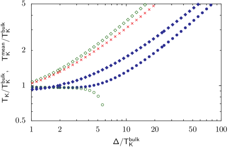
Figure 1: (Color online) Kondo temperature $T_{K}$, for the clean system ($N_{C}$ even $\circ$, $N_{C}$ odd $\bullet$) and average Kondo temperature $T_{K}^{\mathrm{mean}}$, for the chaotic system ($N_{C}$ even $\lozenge$, $N_{C}$ odd $\blacklozenge$, $\mu=0$ $\times$), as functions of $\Delta/T_{K}^{\mathrm{bulk}}$.

IV.1 Kondo temperature

Within the mean-field approximation, the Kondo temperature $T_{K}$ characterizes a transition between a high temperature phase, where the effective hybridization $r$, vanishes, and a low temperature phase with $r\neq 0$. More accurate methods would rather describe a crossover, around $T_{K}$, between weakly and strongly coupled regimes. Despite the oversimplified description of the $T>T_{K}$ weakly coupled regime, the mean-field approximation provides a good estimation for $T_{K}$, and a good description of the physical properties in the $T<T_{K}$ strongly coupled regime. hewson Using Eqs. (8, 11, 12), we find the well known Nagaoka-Suhl equation nagaoka65 for $T_{K}$

$$\frac{2}{J_{K}}=\sum_{l}\frac{\left|A_{l}\right|^{2}}{\varepsilon_{l}-\mu}\tanh\left(\frac{\varepsilon_{l}-\mu}{2T_{K}}\right)\,.$$ (14)

In the bulk limit $\Delta/W\rightarrow 0$, one obtains the relation hewson

$$T_{K}^{\mathrm{bulk}}\approx 1.13\sqrt{W^{2}/4-\mu^{2}}\,\exp\left(-W/J_{K}\right)\,.$$ (15)

In the following, we use $T_{K}^{\mathrm{bulk}}$, rather than $J_{K}$, as the reference energy scale characterizing the Kondo coupling.

The Kondo temperature probability distribution, $p(T_{K})$, is studied by solving Eq. (14) for various realizations. The result is mostly a regular, smooth function, which is depicted in the main part of Fig. 2. In addition to the data shown, there is a non-vanishing contribution $p(T_{K}=0)$ for $N_{C}$ even that is analyzed in the inset of Fig. 2. Note that $T_{K}^{\mathrm{mean}}$ is the average Kondo temperature computed from the regular part of $p(T_{K})$ only.

Figure 1 shows $T_{K}^{\mathrm{mean}}$ for a chaotic system as a function of $\Delta/T_{K}^{\mathrm{bulk}}$, compared to the clean system, each for an even and odd electronic filling of the dot. In the bulk limit ($\Delta/T_{K}^{\mathrm{bulk}}\rightarrow 0$), the Kondo temperatures for even and odd $N_{C}$ coincide as expected, while there is a pronounced parity effect for increasing $\Delta/T_{K}^{\mathrm{bulk}}$, i.e., smaller systems and/or decreasing Kondo interaction strength. For the clean system, $T_{K}$ vanishes in the even case at the critical value $\Delta/T_{K}^{\mathrm{bulk}}\approx 6.28$. mucciolo In all other cases and for larger values of $\Delta/T_{K}^{\mathrm{bulk}}$, the (average) Kondo temperature scales with the level spacing $\Delta$, which becomes, in this limit, the only energy scale of the problem.

The inset of Fig. 2 shows the fraction $P_{0}$ of unscreened impurities at $T=0$ as a function of $\Delta/T_{K}^{\mathrm{bulk}}$. We find that it is always possible to form the Kondo singlet in the odd case (no unscreened impurities), since the chemical potential coincides with an energy level. In the even case, the Kondo effect disappears, on average, with increasing mean level spacing $\Delta$, $P_{0}\rightarrow 1$.

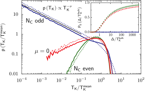
Figure 2: (Color online) Kondo temperature distribution for a chaotic system with $\Delta/T_{K}^{\mathrm{bulk}}=2$ (solid lines), $100$ (dashed lines) for fixed $N_{C}$ and $\mu=0$. For $N_{C}$ odd we see a power law $p(T_{K})\propto T_{K}^{-\nu}$, indicated by the straight line. Inset: probability for vanishing $T_{K}$ in a chaotic system as function of $\Delta/T_{K}^{\mathrm{bulk}}$ for $N_{C}$ even ($\lozenge$), $N_{C}$ odd ($\blacklozenge$), and $\mu=0$ ($\times$).

The parity effects visible in $T_{K}^{\mathrm{mean}}$ are even more dramatic in the probability distribution $p\left(T_{K}\right)$ shown in Fig. 2 for $\Delta/T_{K}^{\mathrm{bulk}}=2$ and $100$. Whereas for $\Delta/T_{K}^{\mathrm{bulk}}=2$ the average Kondo temperatures are almost the same, there is already a significant difference in $p\left(T_{K}\right)$. Most remarkable is a power law scaling, $p\left(T_{K}\right)\propto T_{K}^{-\nu}$, over several orders of magnitude in the odd case. Its existence was pointed out previously miranda ; mucciolo ; cornaglia06 for a related system, the Kondo disorder model (KDM). The KDM describes a Kondo impurity in a bulk electronic bath for which disorder can be included continuously. The chaotic Kondo box that we consider here can in many respects be considered as a KDM with a non-tunable, i.e., fixed, disorder strength. Instead, another parameter can be tuned, $\Delta/T_{K}^{\mathrm{bulk}}$, allowing for a continuous connection between the bulk, $\Delta/W=0$, and the mesoscopic, $\Delta\sim T_{K}^{\mathrm{bulk}}$ regimes. Using Eq. (14) we can show analytically that the power law scaling of $p\left(T_{K}\right)$, with the constant exponent $\nu=1/2$, is a direct consequence of the Porter-Thomas distribution of the intensities $\left|A_{l}\right|^{2}$. It persists for $\Delta\geq T_{K}^{\mathrm{bulk}}$ and is in agreement with Cornaglia et al..cornaglia06 In the case of even occupation, a linear probability distribution, $p\left(T_{K}\right)\sim T_{K}$ was found for small $T_{K}$, mucciolo which is also consistent with our results. For values $\Delta<T_{K}^{\mathrm{bulk}}$ the level structure is no longer important, so all the probability distributions are similar to a Gaussian around $T_{K}^{\mathrm{mean}}$.

IV.2 Magnetic susceptibility

Within the mean-field approximation, the Kondo spin static susceptibility

$$\chi_{0}\left(T\right)\equiv\frac{1}{3}\int_{0}^{1/T}d\tau\langle{\bf S}\left(\tau\right)\cdot{\bf S}\left(0\right)\rangle\,,$$ (16)

reads

$$\chi_{0}\left(T\right)=T\sum_{i\omega_{n}}G_{\mathrm{ff}}\left(i\omega_{n}\right)G_{\mathrm{ff}}\left(-i\omega_{n}\right)\,.$$ (17)

In the decoupled phase, $T>T_{K}$, we recover a Curie law $\chi_{0}\left(T\right)=1/4T$, which characterizes a free spin $1/2$. In order to describe the screening in the Kondo phase $T<T_{K}$, we analyse the local effective moment $T\,\chi_{0}\left(T\right)$, which is equal to $1/4$ for a free spin, and vanishes for a fully screened state. Figure 3 (upper panels) shows the local effective moment for fixed $N_{C}$ as well as for $\mu=0$ at $\Delta/T_{K}^{\mathrm{bulk}}=2$. The clean system (circles) shows parity effects as expected. italians In the odd case, the impurity spin is fully screened at $T=0$, while in the even case it remains unscreened or partially screened for all temperatures. In the chaotic system the average $T\,\chi_{0}$ only slightly differs from the clean case, since the screening of the impurity spin is closely related to the number $N_{C}$ of dot electrons. More information provides the probability distribution $p\left(T\,\chi_{0}\right)$, showing that in the odd case the impurity is screened at $T=0$ for all configurations in the Kondo regime. For $N_{C}$ even all values between $0$ and $1/4$ are taken as $T\rightarrow 0$. This characteristic parity dependence in $p\left(T\chi_{0}\right)$ should be directly accessible in experiments. The $\mu=0$ case contains both features: an increased probability for a screened impurity and a non-vanishing probability for having an unscreened impurity.

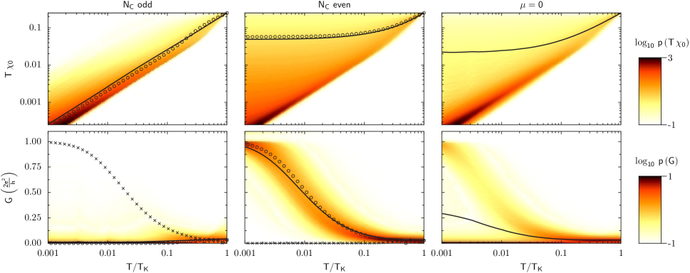
Figure 3: (Color online) Distributions of the local effective moment $T\,\chi_{0}$, (upper panels) and the conductance $G$, (lower panels) for $N_{C}$ odd (left), $N_{C}$ even (center) and $\mu=0$ (right) as functions of $T/T_{K}$. Here, we use $\Delta/T_{K}^{\mathrm{bulk}}=2$. The clean system is symbolized by the circles ($\circ$), the solid lines mark the chaotic average values.
Local effective moment: A broad distribution of values in the $N_{C}$ even case is contrasted with the more confined distribution for $N_{C}$ odd. This pronounced parity effect is directly related to the formation of the Kondo singlet.
Conductance: The probability distribution of the conductance at zero bias voltage shows clear parity effects. The conductance for the non-interacting case ($J_{K}=T_{K}^{\mathrm{bulk}}=0$) is represented by the stars ($\times$), showing that the parity is switched by one, due to the Kondo impurity effective contribution.

IV.3 Conductance

Here, we consider the chaotic Kondo box connected to two leads, denoted by $\alpha=L,R$. We study the tunneling conductance through the box in the linear response regime. The Hamiltonian of the full system is obtained from the Kondo box Hamiltonian (1) by

$$H\mapsto H+\sum_{k\sigma\alpha}\varepsilon_{k}c_{k\sigma\alpha}^{\dagger}c_{k\sigma\alpha}+\sum_{lk\sigma\alpha}\left(t_{lk}^{\alpha}d_{l\sigma}^{\dagger}c_{k\sigma\alpha}+\mathrm{h.c.}\right)\,$$ (18)

where the second term describes the $c-$electrons of the leads and the third term the dot-lead coupling. The leads are assumed to be ideal metals, therefore, the tunneling couplings do not depend on the momentum $k$, $t_{lk}^{\alpha}=t_{l}^{\alpha}$. In order to mimic the chaotic nature of the Kondo box, we also assume that the tunneling couplings are randomly distributed, with second moments $\langle t_{l}^{\alpha}t_{l^{\prime}}^{\alpha^{\prime}}\rangle=t^{2}\delta_{ll^{\prime}}$ (here, $\delta$ denotes the Kronecker symbol, and $t$ is a characteristic tunneling energy). In the presence of a finite bias voltage between the leads $V$, the current through the Kondo box is meirwingreen

$$J(V)=\frac{2e}{h}\int d\omega\left[f_{R}\left(\omega\right)-f_{L}\left(\omega\right)\right]\,\mathrm{Im}\left[\mathrm{Tr}\left\{\mathbf{\Gamma G}\right\}\right]\,,$$ (19)

where $f_{R/L}=f\left(\omega\pm eV/2\right)$ is the Fermi function in the leads, and ${\bf G}$ is the Green’s function matrix of the dot electrons, in the presence of the leads.

$$\Gamma_{ll^{\prime}}^{\alpha}\equiv 2\pi\sum_{k}\rho\left(\varepsilon_{k}\right)t_{lk}^{\alpha}t_{kl^{\prime}}^{\alpha}$$ (20)

is the tunneling matrix, where $\rho$ denotes the density of states of the leads. Hereafter, we approximate the tunneling matrix by its average value, $\Gamma_{ll^{\prime}}^{\alpha}\approx\gamma\delta_{ll^{\prime}}$, where $\gamma\sim\rho t^{2}$. A fully self-consistent mean-field treatment of the system with a finite bias voltage would require to take into account the renormalization of the mean-field parameters, in the presence of the leads, similarly to the approach of Aguado et al.. Aguado Here, we consider the linear response regime, $V\to 0$, as well as the tunneling limit, $\gamma\to 0$. The mean-field parameters $r$, $\lambda$ and $\mu$ are thus not modified by the leads. Furthermore, within the mean-field approximation, the effective Kondo box Hamiltonian (7) is non-interacting. Therefore, the Dyson equation for ${\bf G}$ reads

$$\mathbf{G}^{-1}=\mathbf{G}_{0}^{-1}-i\mathbf{\Gamma}\,,$$ (21)

where the Kondo box (i.e. without the leads) $d-$electron Green’s function ${\bf G}_{0}$ is given by Eq. (13).

The conductance $G=dJ/dV$ is shown in Fig. 3 (lower panels) as a function of $T/T_{K}$. There are clear parity effects: for $N_{C}$ even, the low temperature limit is $G=1$ (in units of the quantum of conductance $2e^{2}/h$), no matter what the underlying realization is. However, for an odd occupation number the conductance goes to $G=0$, since the Kondo singlet blocks the transport channel. The low temperature limit for $\mu=0$ depends on the distance between the chemical potential $\mu$ and the closest energy level.

V Conclusions

We have presented a mean-field approach to the mesoscopic Kondo box problem that allows a very efficient computation of all physical quantities of interest – $T_{K}$, $\chi_{0}$, and $G$ – that are easily, and on an equal footing, accessed via the one-body Green’s functions. In contrast to other methods, we are able (i) to reach very low temperatures $T\sim 0.001\,T_{K}$ within reasonable computation time and (ii) to calculate the probability distributions based on a large number (at least $50\,000$) of realizations of the chaotic Kondo box. Our results agree with those of other approaches when available. Concretely, we find deviations from the bulk system to occur in form of pronounced parity effects. For realizations with an odd number of dot electrons, we confirm and refine the power law distribution of $p\left(T_{K}\right)$. The significant parity effects in the magnetic susceptibility and the conductance provide the basis for a direct comparison with experiments. For example, the expected spread in the experimental values in quantum dots with a certain (even or odd) number of electrons, fixed via Coulomb blockade, will be either large or small, and is therefore already accessible by measuring few samples.

- (1) A.C. Hewson, The Kondo effect to Heavy Fermions, Cambridge University Press (1993).
- (2) D. Goldhaber-Gordon et al., Nature 391, 156 (1998).
- (3) S.M. Cronenwett, T.H. Oosterkamp, L.P. Kouwenhoven, Science 281, 540 (1998).
- (4) J. Nygård, D.H. Cobden, and P.E. Lindelof, Nature (London) 408, 342 (2000).
- (5) R. Egger, Nature Phys. 5, 175 (2009); T. Delattre et al., Nature Phys. 5, 208 (2009);
- (6) W.B. Thimm, J. Kroha, J. von Delft, Phys. Rev. Lett. 82, 2143 (1999).
- (7) P. Simon, and I. Affleck, Phys. Rev. Lett. 89, 206602 (2002).
- (8) P. Simon, and I. Affleck, Phys. Rev. B 68, 115304 (2003).
- (9) G. Franzese, R. Raimondi, and R. Fazio, Europhys. Lett., 62, 264 (2003).
- (10) P.S. Cornaglia, C.A. Balseiro, Physica B 320, 362 (2002).
- (11) Y. Nakamura, Yu.A. Pashkin, and J.S. Tsai, Nature (London) 398, 786 (1999).
- (12) K. Park, V.W. Scarola, and S. Das Sarma, Phys. Rev. Lett. 91, 026804 (2003).
- (13) G. Montambaux, Eur. Phys. J. B 1, 377 (1998).
- (14) E. Miranda and V. Dobrosavljević, Phys. Rev. Lett. 86, 264 (2001).
- (15) S. Kettemann and E.R. Mucciolo, PRB 75, 184407 (2007).
- (16) P.S. Cornaglia, D.R. Grempel, and C.A. Balseiro, Phys. Rev. Lett. 96, 117209 (2006).
- (17) P.W. Anderson, J. Phys. C: Solid St. Phys., 3, 2436 (1970).
- (18) J.E. Hirsch and R.M. Fye, Phys. Rev. Lett. 56, 2521 (1986).
- (19) K.G. Wilson, Rev. Mod. Phys. 47, 773 (1975).
- (20) R. Bulla, T.A. Costi, and T. Pruschke, Rev. Mod. Phys. 80, 395 (2008).
- (21) N. Grewe and H. Keiter, Phys. Rev. B 24, 4420 (1981).
- (22) N.E. Bickers, Rev. Mod. Phys. 59, 845 (1987).
- (23) R.K. Kaul, D. Ullmo, S. Chandrasekharan, H.U. Baranger, Europhys. Lett., 71, 973 (2005).
- (24) A. Yoshimori and A. Sakurai, Prog. Theor. Phys. 46, 162 (1970); P. Coleman, Phys. Rev. B 29, 3035 (1984).
- (25) R. Aguado, and D.C. Langreth, Phys. Rev. Lett. 85, 1946 (2000).
- (26) M.L. Mehta, Random Matrices, Academic (1991).
- (27) M.V. Berry, J. Phys. A: Math. Gen. 10 2083 (1977).
- (28) Y. Nagaoka, Phys. Rev. 138, A1112 (1965); H. Suhl, Phys. Rev. 138, 515 (1965).
- (29) Y. Meir and N.S. Wingreen, Phys. Rev. Lett. 68, 2512 (1992).