The $UV$–Optical Color Dependence of Galaxy Clustering in the Local Universe.

Abstract

We measure the UV-optical color dependence of galaxy clustering in the local universe. Using the clean separation of the red and blue sequences made possible by the $NUV-r$ color-magnitude diagram, we segregate the galaxies into red, blue and intermediate “green” classes. We explore the clustering as a function of this segregation by removing the dependence on luminosity and by excluding edge-on galaxies as a means of a non-model dependent veto of highly extincted galaxies. We find that $\xi(r_{p},\pi)$ for both red and green galaxies shows strong redshift space distortion on small scales – the “finger-of-God” effect, with green galaxies having a lower amplitude than is seen for the red sequence, and the blue sequence showing almost no distortion. On large scales, $\xi(r_{p},\pi)$ for all three samples show the effect of large-scale streaming from coherent infall. On scales $1h^{-1}{\rm\,Mpc}<r_{p}<10h^{-1}{\rm\,Mpc}$, the projected auto-correlation function $w_{p}(r_{p})$ for red and green galaxies fits a power-law with slope $\gamma\sim 1.93$ and amplitude $r_{0}\sim 7.5$ and $5.3$, compared with $\gamma\sim 1.75$ and $r_{0}\sim 3.9h^{-1}{\rm\,Mpc}$ for blue sequence galaxies. Compared to the clustering of a fiducial $L^{*}$ galaxy, the red, green, and blue have a relative bias of $1.5$, $1.1$, and $0.9$ respectively. The $w_{p}(r_{p})$ for blue galaxies display an increase in convexity at $\sim 1h^{-1}{\rm\,Mpc}$, with an excess of large scale clustering. Our results suggest that the majority of blue galaxies are likely central galaxies in less massive halos, while red and green galaxies have larger satellite fractions, and preferentially reside in virialized structures. If blue sequence galaxies migrate to the red sequence via processes like mergers or quenching that take them through the green valley, such a transformation may be accompanied by a change in environment in addition to any change in luminosity and color.

1 Introduction

With the advent of the Sloan Digital Sky Survey (SDSS;York et al. 2000) and its value added galaxy catalogs, it has been possible to study the subject of galaxy bimodality and its relationship to fundamental properties, such as stellar mass and star-formation history (e.g., Kauffmann et al., 2004; Schiminovich et al., 2007; Salim et al., 2007). The broad division of galaxies into star forming disks and quiescent early type galaxies is the fundamental principle of Hubble’s tuning fork system of classification and is well established. In a plot of optical $g-r$ color vs $M_{r}$, red galaxies define a clear sequence, while the locus of blue galaxies is broadened into the so-called ”blue cloud”. The red sequence has been shown to maintain its integrity with look-back time (Bower et al., 1992) and has grown in mass since redshift $\sim 1$. Studies by Bell et al. (2004), Blanton (2006), Faber et al. (2007), and Brown et al. (2008) argue that the stellar mass contained within the red population has increased by roughly a factor of two in half the Hubble time.

A significant breakthrough in expressing this blue/red dichotomy occurred when photometry from the Galaxy Evolution Explorer (GALEX ), notably the near-ultra violet ($NUV$) band, was matched with SDSS photometry (Martin et al., 2007; Wyder et al., 2007; Schiminovich et al., 2007; Salim et al., 2007). When the diagram is plotted using $NUV-r$ as the color, two clear sequences emerge: the familiar red sequence and a new blue sequence in place of the ”blue cloud” of optical studies. Between the blue and red sequences there are galaxies present in a so-called “green valley”. Many of these are spectroscopically classified Type II active galactic nuclei (Rich et al., 2005; Martin et al., 2007; Salim et al., 2007).

Faber et al. (2007), Martin et al. (2007), and Schiminovich et al. (2007) propose several paths by which galaxies might transition from the blue to the red sequence. The presence of AGN in the green valley suggests that AGN activity is associated with a quenching of star formation (Silk & Rees, 1998; Hopkins et al., 2006, 2007). Other paths from the blue to the red sequence might, hypothetically, involve gas-rich mergers of blue galaxies (Toomre & Toomre, 1972), or virial shock heating of cold gas streams (Dekel & Birnboim, 2006). The red sequence might consolidate in luminosity via dissipationless mergers of red galaxies, or low luminosity blue galaxies might acquire bulges through mergers with starbursts, retaining sufficient mass to land the evolved galaxy on the red sequence. However, the green valley might also be populated by casual visitors — red galaxies that acquire gas and form stars or feed a central AGN. Following this brief burst of star formation, these galaxies might ultimately return to the red sequence from which they started.

In Salim et al. (2007), a plot of mass against specific star formation rate reveals a clear division between lower mass, star forming, blue sequence galaxies, and more massive AGN, which are not detected in large numbers until stellar mass $M\sim 3\times 10^{10}M_{\odot}$. The process responsible for populating the green valley and for potentially contributing to evolution from blue to red must bear some relationship to environment and to the dark matter halos in which the galaxies reside. In this study, we investigate the clustering environment of the blue and red sequences, and for the green valley.

The current paradigm of structure formation assumes that galaxies are assembled in dark-matter halos. The dependence of the clustering on galaxy properties may provide clues to the baryonic processes that are important to galaxy formation and evolution. The dependence of galaxy clustering on galaxy type has been known since the earliest studies of extragalactic astronomy (Hubble, 1936; Zwicky et al., 1968). In the modern era of large-scale galaxy surveys, Davis & Geller (1976) showed that the angular auto-correlation of ellipticals has a steeper power-law slope that those of spirals. Recent redshift surveys using the Two-Degree Field Galaxy Survey (2dF) and SDSS confirms these earlier results and the apparent bimodal nature of galaxy clustering (Madgwick et al., 2003; Budavari et al., 2003; Zehavi et al., 2005; Li et al., 2006a; Wang et al., 2007).

Studies using SDSS have further revealed that galaxy color is the property most predictive of local environment. Blanton et al. (2005b) found that at fixed luminosity and color, density does not correlate with surface brightness nor the Sersic index, and argue that morphological properties of galaxies are less closely related to environment than their star-formation history, and are traced by broadband optical colors. (See Park et al. (2007) for an alternative analysis and point of view.) Li et al. (2006a) found that the dependence of clustering on optical $g-r$ color and $D_{4000}$ is much stronger than structural parameters like concentration and surface brightness, and extend to $5h^{-1}{\rm\,Mpc}$, beyond what is expected from the localized halo paradigm of structure formation. They concluded that at fixed stellar mass, the clustering properties of the surrounding dark matter haloes are correlated with the color of the selected galaxies. They further argued that different physical processes may be required to explain environmental trends in star formation, distinct from those established by galaxy structure.

In this paper, we will consider the color dependence of the two-point physical correlation function of galaxies using samples constructed from GALEX , augmented with redshift and optical data from SDSS. In particular, we use the natural separation from the $NUV-r$ color to assign galaxies into three subsamples of red, green and blue galaxies. Our study complements recent work by Heinis et al. (2009) who investigate the physical clustering of galaxies as a function of star-formation history in the local universe, as well as earlier studies by Milliard et al. (2007), Heinis et al. (2007) and Basu-Zych et al. (2008) who investigate the angular-correlation function of rest frame $UV$-selected galaxies and their evolution. We measure the auto-correlation function each of the different subsamples of galaxies, as well as the cross-correlation function between the subsamples. In section 2, we describe in detail the data used in this analysis. In section 3 we describe the method for estimating correlation functions. We present our results in section 4, and discuss their implications for the nature of green valley galaxies and the formation of red sequence galaxies. We summarize our findings in section 6.

2 Data

2.1 GALEX and SDSS Data

The ultraviolet imaging portion of the data-set is from the Galaxy Evolution Explorer Satellite (GALEX ) that was launched in 2003 April (Martin et al., 2005; Morrissey et al., 2005, 2007). GALEX obtains wide field imaging in both the far-UV ($FUV$; centered at $1540$Å) and the near-UV ($NUV$, $2300$Å) over a $1.2^{\circ}$ diameter field of view, with $5^{\prime\prime}$ images. Here we use data from the Medium Imaging Survey (MIS); these images are $\approx 1500$ sec in duration reaching $NUV\approx 23$ mag, covering an orbital shadow crossing. The MIS pointing that defines our sample targets the North Galactic Cap, which overlaps the SDSS spectroscopic footprint; this part of the program was designed from studies cross-matching SDSS and GALEX data. The data-set used for our current analysis is from the Galaxy Release 3 (GR3) which is available from the Multi-mission Archive at STScI (MAST). The GALEX pipeline uses SExtrator (Bertin & Arnouts, 1996) to detect sources and measure fluxes. We use the “MAG_AUTO” output from SExtrator as our default flux measurement; it is essentially a Kron (1980) magnitude with an elliptical aperture.

Because our analysis requires each galaxy to have a spectroscopic redshift, we start our cross-matching with a galaxy from the SDSS Main spectroscopic survey. For each SDSS galaxy, we search for the closest GALEX detection within $4\arcsec$ radius from the location of the SDSS spectroscopic fiber. Only GALEX sources within $0.55^{\circ}$ of the tile center field-of-view (FOV) are retained, since astrometry degrades toward the periphery of the FOV (a problem which will be resolved in later releases) and the incidence of artifacts increases as well. After the matching of GALEX and SDSS sources, we further trim the sample to create a statistically complete data-set following the procedure of Wyder et al. (2007). We will refer the reader to their table 1 for the full details. Here, we list a few essential parameters and the minor modifications we employed: $14.0<r<17.6$, $0.03<z<0.25$, $\sigma_{r}<0.2$, $z_{\rm conf}>0.67$, GALEX exposure time $t>750$s and $16.0<NUV<23.0$. All magnitudes are AB magnitudes and corrected for Galactic foreground extinction.

2.2 SDSS Large-Scale Structure Sample

Considerable effort has been invested by the SDSS team to prepare the redshift data for large-scale structure studies. This secondary data-set known as the New York University Value Added Catalog (NYU-VAGC) is documented in Blanton et al. (2005a) and available from the NYU website. Proprietary versions of this catalogue have been used by many groups within the SDSS collaboration for various investigations of clustering and luminosity function of galaxies. We match the GALEX -SDSS catalog constructed above with the SDSS large-scale structure (LSS) DR5 sample. The version used for our analysis includes all of the detailed radial and angular selection functions for the various statistical subsamples used in previous analyses (e.g. Zehavi et al., 2005). This sample is ideal because we can compare our result with that of Zehavi et al. (2005) which was based solely on selection from optical criteria.

2.3 GALEX –SDSS Overlapping Footprint

In order to statistically define our combined GALEX –SDSS survey, we need to have the understanding of the angular sampling function of the two surveys, which varies across different regions of the sky. GALEX ’s Medium Imaging Survey (MIS) survey consists of overlapping circular tiles (radius $0.55^{\circ}$), while the SDSS spectroscopic survey is a combination of circular spectroscopic plates, but with fiber placement based on a rectangular imaging survey that runs along great circles. To combine the footprints of both surveys, we use the GESTALT footprint server. GESTALT uses a hierarchical pixelization system, enabling one to encode observations of arbitrary geometry while tagging information about completeness and the masking of artifacts. We first encode the GALEX MIS survey using GESTALT. We then obtain the detailed observational footprint of the SDSS Large-scale structure sample from the NYU-VAGC website. The SDSS footprint is expressed as a set of disjoint polygons using the software MANGLE (Hamilton & Tegmark, 2002) which takes into account the complex angular mask and geometry of the SDSS survey. We convert these polygons into the pixelization scheme of GESTALT and consider the intersection of the two surveys. There are approximately 490 square deg in the GALEX –SDSS overlapping footprints after masking for holes, bright stars and satellite trails, and excluding defects.

In order to measure the correlation function, a random sample needs to be constructed to normalize the galaxy pair counts. Angular sampling completeness as a function of position in the sky encoded in the footprint server is used to generate random samples of density roughly 50 times the galaxy density. We adopt the method proposed by Li et al. (2006a) where we assign each galaxy in our sample to a random position on the sky but keep all other attributes the same (e.g. redshift, color, magnitude). This random sample by construction has the same redshift distribution as the original sample, and thus does not smooth out the redshift structure like those generated via the luminosity function. As noted in Li et al. (2006a), this approach works well in surveys with a wide-angular sky coverage (e.g. much larger than the typical large-scale structure), and with small variation in survey depth. We note here that our random sample would inherit the redshift correlation function of the color-magnitude distribution of the parent galaxy sample, only spatial distribution has been randomized, hence any excess in clustering must be due to positional differences.

In the SDSS spectroscopic survey, no two galaxies with separation $\theta$ less than $55\arcsec$ can both be assigned spectroscopic fibers for observation on any given observing plate. Hence, a large fraction of galaxy pairs with $\theta<55\arcsec$ are missing. We correct for this “fiber-collision” problem by using the observed angular correlation function, a method first suggested Li et al. (2006a), and described in detail in the companion paper by Heinis et al. (2009). In brief, the observed projected two-point angular correlation function for both the photometric sample $w_{\rm ph}(\theta)$ and the spectroscopic sample $w_{\rm sp}(\theta)$ are measured and used to construct the pair weighting ratio:

$$F(\theta)=\frac{w_{\rm ph}(\theta)+1}{w_{\rm sp}(\theta)+1}$$ (1)

as a function of separation. Empirically, Heinis et al. (2009) finds $F(\theta)\sim 3$ for $\theta<55\arcsec$ and zero otherwise for the all GALEX –SDSS cross-matched galaxies. We apply this correction to each of the red, green and blue subsamples equally.

3 Methodology

3.1 The Two-point Correlation Function

In brief, the two-point auto-correlation function $\xi(r)$ measures the excess probability of finding a galaxy pair with separation $r$ from a random galaxy distribution,

$$dP=n[1+\xi(r)]dV$$ (2)

where $n$ is the mean number density of galaxy sample. For the last forty years, the correlation function has served as the primary method for cosmologists to quantify the clustering properties of galaxies from large scale surveys (Totsuji & Kihara, 1969; Peebles, 1980). If the underlying density distribution is Gaussian, then the correlation function fully describes all statistical properties of a given distribution. Since early cosmological models are often based on primordial Gaussian dark matter density fields, the use of the correlation function leads to a straightforward comparison between empirical studies on the statistical distribution of galaxies with such models. Recently, with the widespread adoption of a standard $\Lambda$-dominated cosmology (Ostriker & Steinhardt, 1995; Riess et al., 1998; Perlmutter et al., 1999; Spergel et al., 2007), the correlation function is used instead to probe the growth of structure in the universe and the range of formation scenarios for varying kinds of galaxies. The correlation length – the amplitude from a power-law correlation function – provides information on the mass of dark-matter halos in which the various galaxies reside, linking observation with theoretical description of structure formation (Bower et al., 2006; Croton et al., 2006)

For a galaxy survey with a well-defined angular selection function, $\xi$ can be estimated using an optimal estimator like the Landy & Szalay (1993) estimator:

$$\widehat{\xi}_{LS}=\frac{DD-2DR+RR}{RR}$$ (3)

where $DD$, $DR$ and $RR$ are normalized counts of galaxy pairs in the data-data, data-random and random-random catalogs. The Landy & Szalay (1993) estimator is preferred because it is relatively insensitive to the size of the random catalog and to edge corrections (Kerscher et al., 2000).

Because we observe galaxies in redshift and projected space and not in physical space, in practice, the correlation function is first measured on a two-dimensional grid of separations: $\pi$ along the line of sight (redshift space) and $r_{p}$ for angular separation on the sky. In addition to providing information about the underlying mass distribution through the amplitude of the clustering signals, the two-dimensional correlation function $\xi(\pi,r_{p})$, contains additional information about the dynamics of the galaxies (Peebles, 1980). At small projected separations $r_{p}$, random motions within virialized over-density (e.g. clusters of galaxies) causes an elongation along the line-of-sight ($\pi$ direction) known as the “finger-of-God” effect. On large scales, coherent streaming of galaxies into potential wells causes an apparent compression of structure along the line-of-sight (Sargent & Turner, 1977; Kaiser, 1987; Hamilton, 1992). Various studies have used $\xi(\pi,r_{p})$ to extract cosmological and dynamical information (e.g., Tinker, 2007).

3.1.1 Real-Space Correlation

Because redshift space distortion only affects the line-of-sight component of $\xi(\pi,r_{p})$, we can recover the true space correlation function $\xi(r)$ by following the standard procedure of computing the projected correlation function:

$$w_{p}(r_{p})=2\int_{0}^{\infty}d\pi\xi(r_{p},\pi).$$ (4)

In practice, we integrate along the line-of-sight direction out to $\pi=30h^{-1}{\rm\,Mpc}$. This is large enough to include almost all correlated pairs but also stable enough to suppress noise from distant uncorrelated pairs. The projected correlation function can in turn be related to the real space correlation function $\xi(r)$,

$$w_{p}(r_{p})=2\int_{0}^{\infty}rdr\xi(r)(r^{2}-r_{p})^{-1/2}.$$ (5)

If the real-space correlation function follows a power-law $\xi(r)=(r/r_{0})^{\gamma}$, we can infer its parameters: the correlation length $r_{0}$ and the power-law slope $\gamma$ from the best-fit power-law to $w_{p}(r_{p})$ using the following deprojection:

$$w_{p}(r_{p})=r_{p}\left(\frac{r_{p}}{r_{0}}\right)^{-\gamma}\Gamma\left(\frac{1}{2}\right)\Gamma\left(\frac{\gamma-1}{2}\right)\,\Bigr{/}\,\Gamma\left(\frac{\gamma}{2}\right).$$ (6)

3.1.2 Cross-correlation

Related to the auto-correlation function is the cross-correlation function between two classes of galaxies. The cross-correlation function $\xi_{1,2}(r)$, measures the clustering of one type of galaxy around another. $\xi_{1,2}(r)$ is essentially the probability of finding a galaxies of type 1 around a galaxy of type 2 as a function of separation $r$. For our analysis, we use the cross-correlation version of the classical Davis & Peebles (1983) estimator:

$$\widehat{\xi}_{1,2}=\frac{D_{1}D_{2}}{D_{1}R_{2}}-1$$ (7)

where $D_{1}D_{2}$ are the normalized counts of cross-pairs; while $D_{1}R_{2}$ are cross-pairs of type 1 with random galaxies having the same redshift distributions as galaxies of type 2.

Recently, the cross-correlation function has been used extensively in clustering studies of galaxy properties (Zehavi et al., 2005; Wang et al., 2007; Coil et al., 2008; Padmanabhan et al., 2008; Chen, 2009) since the auto-correlation function alone tells us little about how galaxies of various types relate to one another. Two populations of galaxies may both have comparable correlation strength, and yet be physically unrelated if they are spatially segregated. Specifically, the cross-correlation function may be used in conjunction with the auto-correlation functions of the galaxies to glean information as to how they mix statistically. For example, if the two populations are well mixed, i.e. they are consistent with being drawn stochastically from their respective auto-correlation function equally, their projected cross-correlation function $w_{p}^{1,2}(r_{p})$ would follow that of the geometric mean of their auto-correlation functions

$$w_{p}^{\overline{1,2}}(r_{p})=\sqrt{w_{p}^{1,1}(r_{p})w_{p}^{2,2}(r_{p})}.$$ (8)

On the other hand, if the populations were segregation between the populations and do not distribute evenly in all space, e.g. they sit on different halos, the amplitude of $w_{p}^{1,2}(r_{p})$ would be lower than that of $w_{p}^{\overline{1,2}}(r_{p})$ known in the literature as stochastic anti-bias (e.g. Blanton, 2000; Swanson et al., 2008)

3.1.3 Bootstrap Errors

We estimate the errors for the correlation measurements using a modified bootstrap (Efron, 1981) method for spatial statistics known as marked-point bootstrap (Loh, 2008). We first estimate the contribution of each galaxy to the correlation function – the marks:

$$\xi_{i}(r)=\sum_{j=1,j\not=i}^{n}\phi\{|x_{i}-x_{j}|\in(r-dr,r+dr)\}$$ (9)

such that

$$\xi(r)=\sum_{i=1}^{n}\xi_{i}$$ (10)

where $n$ is the number of galaxies and $\phi$ is the chosen correlation estimator (e.g. $\widehat{\xi}_{LS}$). Hence, the mark $\xi_{i}$ associated with galaxy $x_{i}$ is the number of excess pairs at a distant $r$ from $x_{i}$. These $\xi_{i}$ are (roughly) independent, and identically distributed, and can be used to replicate $B$ bootstrap samples by the sampling with replacement. An estimate of the correlation function $\widehat{\xi_{j}^{*}}$ can be computed from each of the $j$-th bootstrap samples. We use $B=999$ bootstrap samples for our analysis. The distribution of $\widehat{\xi^{*}}(r_{i})$ can be use to estimate the error bars of the correlation function at each separation $r_{i}$. For an equivalent of one sigma errors, we ranked $\widehat{\xi^{*}}(r_{i})$ and take the $159^{nd}$ and $840^{th}$ for the lower and upper error bounds. Because the $\widehat{\xi}$ errors for the $r_{i}$ are correlated, when we estimate parameters for the two parameter power-law model (equation 6), we refitted each bootstrap sample to obtain a two dimension distribution of the parameters.

We chose this method over the conventional jackknife methods because of the fragmented nature of the GALEX –SDSS footprint. Our bootstrap errors are consistent with the jackknife errors estimated by excluding one GALEX tile at a time. We note here that jackknife errors are known to overestimate the variance on small-scale, and often bias the overall correlation estimates (Norberg et al., 2009). Since bootstrap is a form of internally estimated errors, and internally estimated errors are known not to reproduce externally estimated errors accurately (Norberg et al., 2009), our clustering results should be treated with caution.

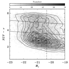
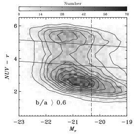
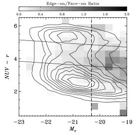
Figure 1: $NUV-r$ vs $M_{r}$ color-magnitude diagram (CMD) of galaxies in the local Universe. The left panel shows the full distribution. The middle panel shows the distribution drawn from face-on galaxies with $b/a>0.6$, used to correct for the effect of dust on the CMD. The right panel shows the distribution of edge-on/face-on ratio overlay onto the CMD contours. The green valley is dominated by region of the CMD with high relative fraction of edge-on galaxies. By limiting ourselve to galaxies with $M_{r}<-20.3$ (dashed vertical lines) for the volume-limited sample, we also eliminate region of the CMD with the highest fraction of edge-on galaxies.

4 Dependence of Clustering on $UV$–Optical Color

Figure 1 shows the $NUV-r$ color-magnitude diagram (CMD) in the local universe. All absolute magnitudes are $k$-corrected using the K_CORRECT program by Blanton & Roweis (2007) and are quoted in units with Hubble constant $H_{\rm 0}=100h{\rm\ km\ s^{-1}\ Mpc^{-1}}$ , i.e. $M_{r}\equiv M_{r}-5\log(h=1)$. Compared with the optical color-magnitude diagram (e.g. $g-r$ vs $M_{r}$), the $NUV-r$ color axis has a higher dispersive power. The scatter plot shows two clear sequences: red and blue, and an intermediate “valley” of “green” population. Conventional optical diagrams only display a single red sequence with an extended blue cloud. Hence, diagnostic diagrams like Figure 1 separate galaxies into three natural groupings: (1) a red sequence of bulge-dominated galaxies with old stellar systems, (2) a blue sequence of star-forming systems consisting of mainly late-type galaxies, and (3) galaxies in a “green valley” that in principle might exhibit transitional properties (Martin et al., 2007; Schiminovich et al., 2007). Detailed luminosity functions and physical properties analysis of these galaxies derived from this $UV$–optical CMD has been reported elsewhere (Wyder et al., 2007; Martin et al., 2007; Salim et al., 2007; Schiminovich et al., 2007). Here, we investigate the clustering properties of these three subpopulations of galaxies, separated by the two tilted horizontal lines, using the two-point auto-correlation function, as well as their relation to each other using the cross-correlation function. Our results are not sensitive to $0.25$ mag shift in the oblique equation used to classify the galaxies.

4.1 Dust

Dust content within each galaxy can modify their broadband colors, hence the resultant color-magnitude diagram, as galaxies move from one group to another (Martin et al., 2007; Schiminovich et al., 2007). This is a concern, as it might affect our estimate of the correlation function by either increasing the scatter between groups, or bias the result in a systematic but unknown manner. Indeed, a fraction of the green valley galaxies are dusty star forming galaxies whose intrinsic color would have placed them on the blue sequence in the absence of dust (Wyder et al., 2007). However, the available procedures for dust correction are highly uncertain. They give inconsistent results depending on whether one uses a primarily photometric approach (Salim et al., 2007; Johnson et al., 2006), or one based on spectroscopic indices (Kauffmann et al., 2004). The former, for example, has the side effect of reducing the red sequence number counts substantially (Schiminovich et al., 2007; Heinis et al., 2009), while the latter approach requires spectroscopy of modest S/N, which is not available for part of our sample. A comprehensive analysis of the clustering as a function of star-formation history with a dust-corrected color-magnitude diagram using the method of Johnson et al. (2006) is done in Heinis et al. (2009).

Here, we adopt a geometric approach. Because dust lanes in galaxies usually appear when viewed edge-on, we can reduce the effect of dust on galaxy color by restricting our analysis to galaxies that are primarily face-on. The middle panel of Figure 1 shows the “dust-corrected” color-magnitude diagram obtained by including only galaxies with isophotal (minor-over-major) axis ratio $b/a>0.6$. To the extent that each of the subpopulations have the same intrinsic distribution of $b/a$, removing edge-on galaxies will give a correct mixture of galaxies that mimic the intrinsic color-magnitude distribution. Comparing the dust-corrected CMD with the CMD on the left panel (hereafter the full distribution), the density of green galaxies around $M_{r}\sim-21$ is reduced substantially, with the contours showing a more pronounced “valley” separating the sequence of galaxies.

The righthand panel of Figure 1 shows the median ratio of edge-on ($b/a<0.4$) to face-on ($b/a>0.8$) as a function of color and magnitude, with the same density contours from the middle panel. The region with the highest edge-on/face-on ratio falls in the green valley and towards the faint end of the luminosity distribution (Choi et al., 2007; Martin et al., 2007; Schiminovich et al., 2007). For the galaxies with the magnitude range with $-23.5<M_{r}<-19.0$ used to construct our flux-limited sample, the median $b/a$ for red and blue sequence galaxies are $0.73$ and $0.72$ respectively, while for green valley galaxies it is $0.66$. Choi et al. (2007) find that edge-on galaxies are also statistically fainter due to the internal extinction, and it affects morphologically late-type galaxies (classified by eye) more than early-type galaxies. Hence by limiting our analysis to face-on galaxies, we would reduce biases associated with differential dimming in addition to the biases from color shifts. Following Choi et al. (2007), we restrict our analysis to galaxies with $b/a>0.6$ as a proxy for a galaxy distribution derived from a dust-corrected CMD.

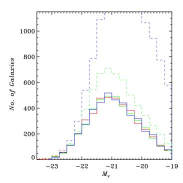
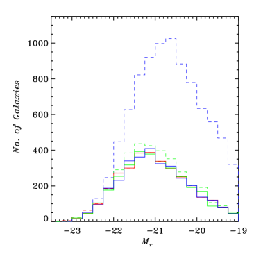
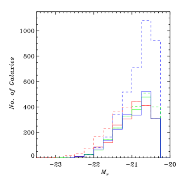
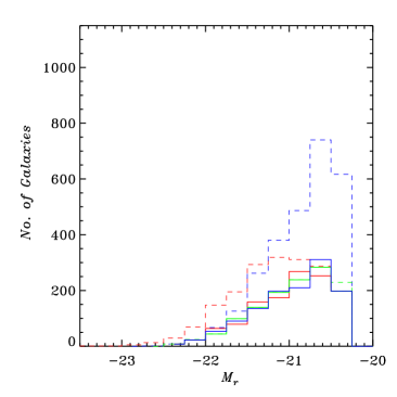
Figure 2: The luminosity distribution of our flux-limited (top row) and volume-limited (bottom row) samples. The two panels on the left are for the full distribution, the right is for dust-corrected CMD, using only galaxies with $b/a>0.6$. The dashed histograms show the original luminosity distribution for each of the subsamples of red, green and blue galaxies. We resampled the luminosity to match the number counts of the minimal of the three distribution at each magnitude bin, shown as solid histograms. Even for the volume-limited samples, the variations in the original luminosity distribution among the three subsamples are substantial. Blue galaxies are heavily weighted towards the less luminous end compared to red or green galaxies.

4.2 Luminosity bias

The clustering of galaxies is luminosity dependent. Norberg et al. (2002), Zehavi et al. (2005) and Li et al. (2006a) show that the amplitude of the projected correlation function $w_{p}$ increases monotonically as a function of luminosity (or stellar mass) on scales ranging from $0.2h^{-1}{\rm\,Mpc}$ to $10h^{-1}{\rm\,Mpc}$. In order to study the color dependence on clustering, or to compare the clustering intrinsic to the membership of discrete subpopulations, it is vital to remove this known luminosity dependence. The top two panels of Figure 2 shows the luminosity distribution of the red, green and blue population of galaxies with $M_{r}<-19$ from our flux-limited sample. The series of dashed histograms (in red, green and blue) show the original luminosity distributions. Blue galaxies are more numerous and less luminous, on average, compare to red and green galaxies, reflecting a steeper blue luminosity function at the faint-end (Wyder et al., 2007). To remove this luminosity dependence, we resample the luminosity histograms to match the number counts of the smallest of the three distributions at each magnitude bin. The result of this resampling is shown by the solid histograms. The left panel shows histograms from the full distribution, while the right shows those from a dust-corrected distribution. There are 4177 (full) and 3148 (dust-corrected) galaxies in each of the resampled luminosity distribution of red, green and blue galaxies, with a common median luminosity of $M_{r}\sim-21.0$, about half a magnitude brighter than $M^{*}$, the typical luminosity (Blanton et al., 2003). Note that if the fundamental attribute that drive clustering is stellar mass, removing the luminosity dependence like what we have done here would still leave residual clustering due to the difference in mass-to-light ratio of the respective color selected sample.

4.3 Volume-limited sample

While the resampled red, green and blue galaxies are matched in luminosity, they are not matched in volume and have different redshift distributions. This makes the interpretation of the physical correlation function problematic. To this end, we select the largest possible volume within our catalog, using a redshift cut of $0.03<z<0.12$ and an additional luminosity cut at $M_{r}<-20.3$ to construct a volume-limited sample. The luminosity distributions of this sample are shown on the bottom row of Figure 2. As before, the left panel is for the full CMD, while the right panel are for the dust-corrected (restricted) CMD. Similar to the flux-limited case, the (original) blue dashed histograms are substantially different the red and the green, and are weighted more heavily towards the faint-end. We resample the histograms to match in luminosity. Note that in the case, the procedure outlined in section 4.2 essentially amounts to looking for an optimal function $W(L)$ such that $W(L)\Phi(L)$ gives the minimum luminosity function of the three subsamples. The new red, green and blue volume-limited subsamples each consists of 1971 (full) and 1226 (dust-corrected) galaxies with a common median luminosity of $M_{r}\sim 20.9$, almost identical to the flux-limited case.

4.4 Red, Green, Blue Auto-correlation

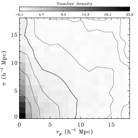
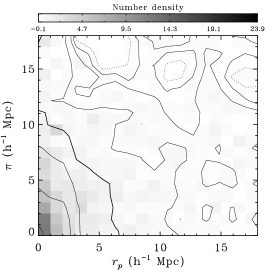
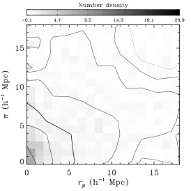
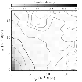
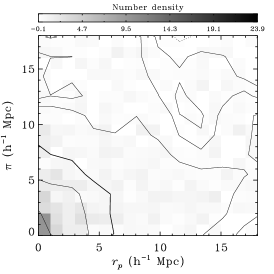
Figure 3: Contours and normalized counts of the two-dimensional correlation function $\xi(\pi,r_{p})$ for red (left), green (middle) and blue (left) populations for the flux-limited sample. The panels on the top row are for the full distribution, bottom row are restricted to face-on galaxies ($b/a>0.6$). The contours obtained after 2 x 2 $h^{-1}{\rm\,Mpc}$ boxcar smoothing. The levels are 0.0 (dotted lines), 0.25, 0.5, 1.0 (heavy lines), 2.0, 4.0, 8.0 and 16.0. Red galaxies have the strongest finger of God effect (extension in the $\pi$ direction). The finger-of-God effect is seen in the green sample as well, while it is not present in the blue. Galaxies in the green valley appear to have clustering characteristics of the red sequence.

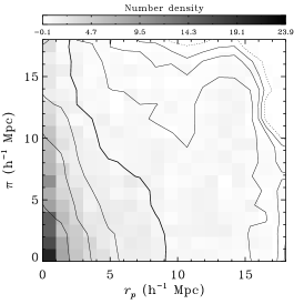
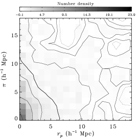
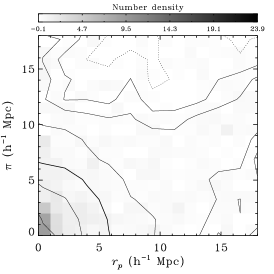
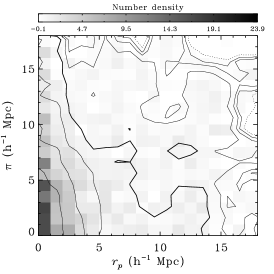
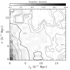
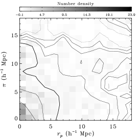
Figure 4: Contours and normalized counts of the two-dimensional correlation function $\xi(\pi,r_{p})$ for red (left), green (middle) and blue (left) populations for the volume-limited sample. The panels on the top row are for the full distribution, bottom panels are restricted to face-on galaxies ($b/a>0.6$). The contours obtained after 2 x 2 $h^{-1}{\rm\,Mpc}$ boxcar smoothing. The levels are 0.0 (dotted lines), 0.25, 0.5, 1.0 (heavy lines), 2.0, 4.0, 8.0 and 16.0. Red galaxies have the strongest finger of God effect (extension in the $\pi$ direction). Similar to Figure 3, but with lower signal-to-noise, the finger-of-God effect is seen in the green sample as well, while it is not present in the blue.

Figure 3 and 4 shows the two-dimensional auto-correlation function $\xi(\pi,r_{p})$ as a function of line-of-sight ($\pi$) and projected ($r_{p}$) separation for the flux-limited and volume-limited samples. The panels on the first row in each figure are from the full distribution, while the second row are from the dust-corrected distribution. The panels are for red sequence (left), green valley (middle) and blue sequence (right) galaxies. We have binned $\pi$ and $r_{p}$ linearly at $1h^{-1}{\rm\,Mpc}$. For all panels, the grey scale has the same range, and the contours are boxcar smoothed at $2h^{-1}{\rm\,Mpc}$. The $\xi(\pi,r_{p})$ contours indicate the constant probability of finding pairs at a given $\pi$ and $r_{p}$. The heavy solid line marks $\xi(\pi,r_{p})=1$, and contours are spaced with increment (inner) and decrement (outer) by a factor of 2. The effect of redshift-space distortion is clearly seen in all panels, manifested by their departure from isotropy (concentric circles). At small $r_{p}$, the contours are elongated along the line-of-sight ($\pi$) due to virial motions of galaxies in clusters. At large $r_{p}$, the contours are compressed in the $\pi$ direction due to the coherent large-scale streaming as galaxy infall into potential well. We recover the results of Zehavi et al. (2005): red sequence galaxies show the strongest finger-of-God effect and the larger correlation amplitude; and all three subpopulations (of all samples and distribution) show clear signs of large-scale compression.

We see a clear finger-of-God effect for green valley galaxies, but not for blue sequence galaxies. In Figure 3, if one compares the first contour inwards from $\xi=1$ (heavy line) for red galaxies to the $\xi=1$ contour of green galaxies, green and red galaxies have identical kinematics, differing only by a scaling in the amplitude. The blue sequence appears to have a dynamical structure dominated by large-scale streaming distinct from both red and green galaxies, similar to the optical blue cloud sample of Zehavi et al. (2005). We will consider the implications of this in the discussion below. The same conclusion can be drawn from the volume-limited sample shown on in Figure 4. The dust-corrected samples (bottom row) is substantially noisier. We also note that the contours of the blue sequence of the volume-limited full sample (top right panel) are roughly circular for $\sim 4<\pi,r_{p}<10h^{-1}{\rm\,Mpc}$ where the finger-of-God elongation is balanced by compression due in infall.

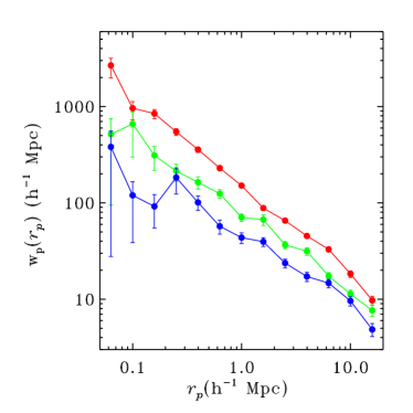
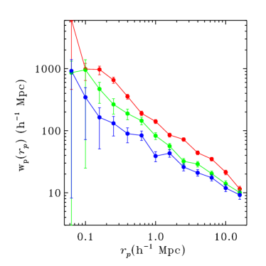
Figure 5: The projected correlation function, $w_{p}(r_{p})$, of red sequence, green valley, and blue sequence galaxies for the flux-limited sample. The left (right) panel is from the full (dust-corrected) distribution. From red to blue, there is an increase in convexity, with the progressive shallowing of the slope on large scales, indicating an excess of two-halo signals at scale ($r_{p}\gtrsim 1h^{-1}{\rm\,Mpc}$).

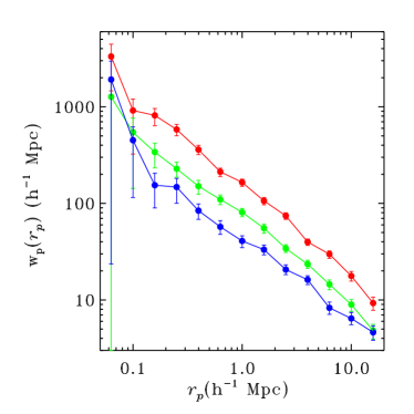
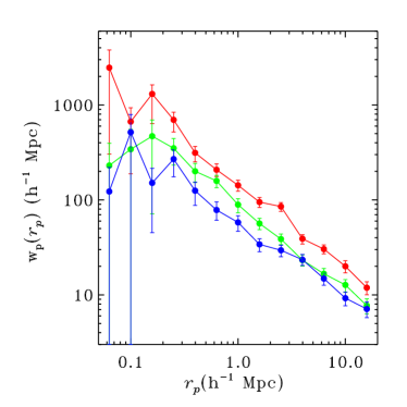
Figure 6: The projected correlation function, $w_{p}(r_{p})$, of red sequence, green valley, and blue sequence galaxies for the volume-limited sample. Similar to Figure 5, from red to blue, there is an increase in convexity, with the progressive shallowing if the slope on large scale, indicating an excess of two-halo signals. at scale ($r_{p}\gtrsim 1h^{-1}{\rm\,Mpc}$). For the full distribution (left panel), the green $w_{p}(r_{p})$ is parallel to the red with a lower amplitude for scales $0.2<r_{p}<10h^{-1}{\rm\,Mpc}$. For the dust-corrected distribution (right panel), the blue $w_{p}(r_{p})$ approaches the green on large scales.

Figure 5 and 6 shows the projected correlation function $w_{p}(r_{p})$ for the flux-limited and volume-limited samples. The colored (red, green, blue) points are the respective measured correlation function. The panel on the left (right) is for the full (dust-corrected) distribution. As expected, in all four panels, the red sample has the largest amplitude, the blue the lowest, and green in between. On large scales ($r_{p}\gtrsim 1h^{-1}{\rm\,Mpc}$), the ratio of projected auto-correlation function of the respective samples are constant as a function of scales, as expected from linear theory. All correlation functions appear to have a form that is well fit by a broken power-law with the dust-corrected distribution having a more pronounce convexity. It is noteworthy that the flux-limited analysis (Figure 5) is more noisy than the volume-limited analysis (Figure 6), despite having a factor of two greater numbers. We believe that this is due to the inclusion of uncorrelated (in redshift space) galaxies, which dilute the clustering signal, especially for blue galaxies on small scales. From here onwards, we will restrict our analysis to the volume-limited sample.

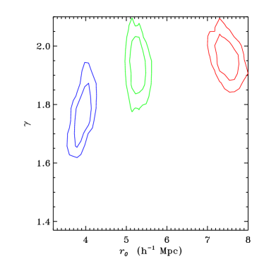
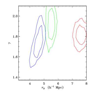
Figure 7: Confidence contours of the power-law fits to $w_{p}(r_{p})$ on scales $1h^{-1}{\rm\,Mpc}<r_{p}<10h^{-1}{\rm\,Mpc}$ for the full (left panel) and dust-corrected (right) distributions from the volume-limited sample. The three colors are for red, green and blue subsamples, with the inner (outer) contours encircling the 68 (95) % confidence region in the $r_{0}$–$\gamma$ space.

When we fit the projected correlation function of the full distribution with the standard two parameter power-law for scales from $1<r_{p}<10h^{-1}{\rm\,Mpc}$, red and green galaxies appears to have similar slope with $\gamma\sim 1.93$, while blue galaxies have a substantially shallower slope, with $\gamma\sim 1.75$. The best fit correlation lengths $r_{0}$ are $7.5h^{-1}{\rm\,Mpc}$ (red), $5.3h^{-1}{\rm\,Mpc}$ (green), and $3.9h^{-1}{\rm\,Mpc}$ (blue). The result of the covariance analysis using 999 bootstrap samples is shown as confidence interval contours – 68% (inner) and 95% (outer) in Figure 7 (left panel). These results are in excellent agreement with Heinis et al. (2009). The correlation function from the dust-corrected distribution is substantially noisier, in part due to the smaller number of galaxies. Applying the same power-law fit, we obtain a larger uncertainty in $\gamma$, but comparable uncertainty in $r_{0}$. This is shown on the right panel of Figure 7 and tabulated in Table 1.

Table 1: Power-law fit to the projected auto-correlation function of volume-limited samples ($1h^{-1}{\rm\,Mpc}<r_{p}<10h^{-1}{\rm\,Mpc}$)

Full-Sample	$N$	$z$	median $M_{r}$	$r_{0}$	$\gamma$	Relative Bias	$\chi^{2}/dof$
Red……….	$1971$	$(0.03,0.12)$	$-20.9$	$7.5\pm 0.27$	$1.94\pm 0.07$	$1.53\pm 0.08$	$1.36$
Green……..	$1971$	$(0.03,0.12)$	$-20.9$	$5.3\pm 0.19$	$1.93\pm 0.08$	$1.08\pm 0.06$	$0.40$
Blue………	$1971$	$(0.03,0.12)$	$-20.9$	$3.9\pm 0.25$	$1.73\pm 0.10$	$0.81\pm 0.06$	$1.54$
Face-On
Red……….	$1226$	$(0.03,0.12)$	$-20.9$	$7.6\pm 0.38$	$1.81\pm 0.11$	$1.47\pm 0.10$	$2.47$
Green……..	$1226$	$(0.03,0.12)$	$-20.9$	$5.5\pm 0.24$	$1.92\pm 0.15$	$1.13\pm 0.09$	$0.48$
Blue………	$1226$	$(0.03,0.12)$	$-20.9$	$4.6\pm 0.31$	$1.74\pm 0.17$	$0.92\pm 0.09$	$1.17$

On the left panel, the projected correlation function of green galaxies is evidently intermediate between the red and the blue on a range of scales ($0.2<r_{p}<6h^{-1}{\rm\,Mpc}$), and runs faithfully parallel with the red correlation function, but with a lower amplitude. The picture for the dust-corrected distribution is slightly different. While the green still runs in between the red and blue for $r_{p}<1h^{-1}{\rm\,Mpc}$ and mostly parallel to the red with a lower amplitude for broad range of scales, for larger scales ($r_{p}\gtrsim 2h^{-1}{\rm\,Mpc}$), it coincides with the blue. This is a consequence of the more prominent two-halo excess on large scales seen in the blue correlation function.

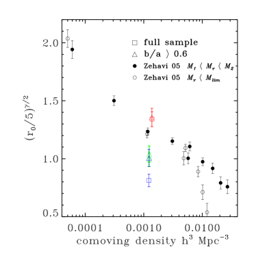
Figure 8: Bias relative to the typical $L^{*}$ galaxy with a $\xi^{fid}(r)=(r/r_{0})^{-1.8}$ at $r_{p}=5h^{-1}{\rm\,Mpc}$ versus co-moving number density. We also plotted points from SDSS (Zehavi et al.2005). The solid circles are from their luminosity range analysis, i.e. galaxy with absolute magnitude between $M_{1}$ and $M_{2}$, while the open circles are from their luminosity threshold analysis, i.e. $M_{r}<M_{lim}$. While far from unique, the higher red bias suggests that on average red galaxies are more likely to be satellite galaxies then a typical galaxy with those number densities. If we assume the lower blue and green galaxies are all central galaxies in the halo they reside in, the lower observed number densities suggest that only a fraction of these halos, as described by their bias, host a blue or green galaxy, as their expected number density is much higher.

One way to compare the clustering between subpopulations of galaxies is through their relative bias (e.g. Norberg et al., 2002), defined as

$$\frac{b_{i}}{b_{*}}(r)=\sqrt{\frac{\xi_{i}(r)}{\xi_{*}(r)}}\simeq\frac{r_{0,i}^{\gamma_{i}/2}}{r_{0}^{\gamma/2}}r^{(\gamma-\gamma_{i})/2}$$ (11)

where $\xi_{i}$ is the correlation function of interest, $\xi_{*}$ is the fiducial correlation function that all correlation function is compare with. The approximate equality holds when the correlation function takes a power-law form. Zehavi et al. (2005) found that a typical $L^{*}$ galaxies in the local universe with $-20<M_{r}<-21$ from the SDSS main spectroscopic sample have a fiducial power-law correlation function with $\xi_{*}(r)=(r/5h^{-1}{\rm\,Mpc})^{-1.8}$ on scale $1<r_{p}<10h^{-1}{\rm\,Mpc}$. By fitting the correlation function using a constant $\gamma=1.8$ on scales $1<r_{p}<10h^{-1}{\rm\,Mpc}$, we obtained the bias relative at $r_{p}=5h^{-1}{\rm\,Mpc}$ to a fiducial $L^{*}$ galaxies for each of our subpopulations: $b_{\tt red}/b_{*}=1.53\pm 0.08$, $b_{\tt green}/b_{*}=1.08\pm 0.06$ and $b_{\tt blue}/b_{*}=0.81\pm 0.06$ for the full-sample, and $b_{\tt red}/b_{*}=1.47\pm 0.10$, $b_{\tt green}/b_{*}=1.13\pm 0.09$ and $b_{\tt blue}/b_{*}=0.92\pm 0.09$ for the dust-corrected samples (Table 1). In Figure 8, we plot $b_{i}/b_{*}(r=5h^{-1}{\rm\,Mpc})=(r_{0}/5h^{-1}{\rm\,Mpc})^{\gamma}$ as a function of the co-moving number density and compare our values with those obtained by Zehavi et al. (2005). Co-moving number density of our sample is estimated using the $1/V_{max}$ method and further corrected to match those obtained by Wyder et al. (2007). While all the samples by construction have almost identical co-moving density, there is a range of relative bias, with the red having the highest bias, and blue the lowest. The spread among the bias are much smaller among the dust-corrected samples. Red galaxies have clustering strength above the nominal strength (inferred from a typical SDSS galaxy) for a given number density. One plausible scenario suggest that red galaxies have a larger than average satellite fraction. On the other hand, blue and green galaxies have lower observed number density compare to their clustering. If we assume all blue and green galaxies are central galaxies in the halo they reside in, the lower observed number densities ($\sim 0.001h^{3}{\rm\,Mpc}^{-3}$) suggest that only a small fraction of these halos, as described by their lower bias, host a blue or green galaxy, as their expected number density (inferred from SDSS to be $\sim 0.01h^{3}{\rm\,Mpc}^{-3}$) is much higher. These fractions are increased if the average phases of green and blue is shorter then the lifetime of the halos (Haiman & Hui, 2001; Martini & Weinberg, 2001). In the case of the green galaxies, the transitional nature of these galaxies may be closely related to the AGN they host, or to minor mergers and starbursts, with triggering cycles corresponding to the duty cycles for these respective phenomena. We defer a more detail analysis of halo occupation and the life cycle of transition galaxies using star-formation rate tracers of different lags to a future paper (Heinis et al. in prep.). Using a theoretical bias function of dark matter halos (Seljak & Warren, 2004) and normalizing to $M_{*}=10^{12}h^{-1}{\rm\,M_{\sun}}$, red galaxies cluster similar to halos with mass $\sim 10^{12.7}h^{-1}{\rm\,M_{\sun}}$, green galaxies $10^{12.2}h^{-1}{\rm\,M_{\sun}}$, and blue galaxies $10^{11.6}h^{-1}{\rm\,M_{\sun}}$.

4.5 Cross-Correlation Functions

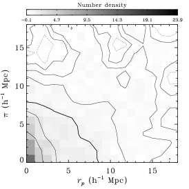
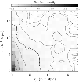
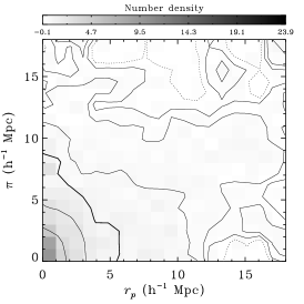
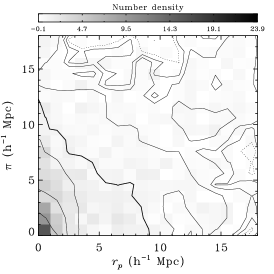
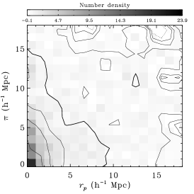
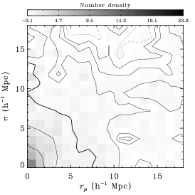
Figure 9: Contours and normalized counts of the two-dimensional cross-correlation function $\xi(\pi,r_{p})$ for red-blue (left), green-red (middle) and green-blue (left) for the volume-limited sample. The panels on the top row are for the full distribution, bottom panels are restricted to face-on galaxies ($b/a>0.6$). The contours obtained after 2 x 2 $h^{-1}{\rm\,Mpc}$ boxcar smoothing. The levels are 0.0 (dotted lines), 0.25, 0.5, 1.0 (heavy lines), 2.0, 4.0, 8.0 and 16.0. The large scale infall effect is seen in all three panels. On small scales, the finger-of-God effect is strongest for the red-green, intermediate for red-blue and weakest for green-blue, as expected. Note that red-blue CCF $\xi(\pi,r_{p})$ has a weaker finger-of-God and stronger infall compression compare to the green valley auto-correlation function (Figure 4 middle panels).

Figure 9 shows the two-dimensional $\xi(r_{p},\pi)$ cross-correlation function (CCF) for the three cross-pairs of galaxies in our volume-limited sample, with the panels on the top for the full distribution, and the bottom panels for the dust-corrected distribution. The large scale infall effect is seen in all three panels suggesting that the galaxies, on average, trace a similar matter distribution as expected from linear theory. On small scales, the finger-of-God effect is strongest for the red-green CCF, intermediate for red-blue and green-blue. In Figure 10 we plot the relative amplitude of $\xi$ at the projected distance $r_{p}=1h^{-1}{\rm\,Mpc}$ as a function of line-of-sight distance $\pi$. The circles are for green-red cross correlation, squares for red-blue, and triangles for green-blue. Green-red have largest amplitude for a wide range of $\pi$, while red-blue and green-blue have smaller amplitudes. The stronger finger-of-god component suggest that the dynamics of red and green are more strongly coupled compared with red-blue or green-blue pairs. Note that red-blue CCF have a very different $\xi(\pi,r_{p})$ compared with the green auto-correlation function (ACF), the former has a weaker finger-of-God and stronger infall compression.

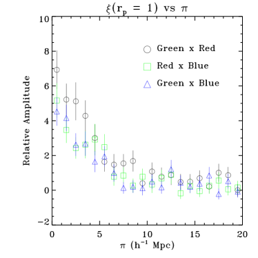
Figure 10: This figure shows the relative amplitude of $\xi$ at projected distance $r_{p}=1h^{-1}{\rm\,Mpc}$ as a function of the line-of-sight distance $\pi$. The circles are for green-red cross correlation, squares for red-blue, and triangles for green-blue. Green-red have largest amplitude for a wide range of $\pi$, while red-blue and green-blue have smaller amplitudes. These results suggest that the finger-of-god component of green-red cross correlation function is stronger then those from red-blue or green-blue.

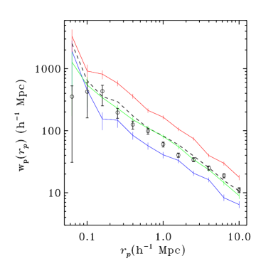
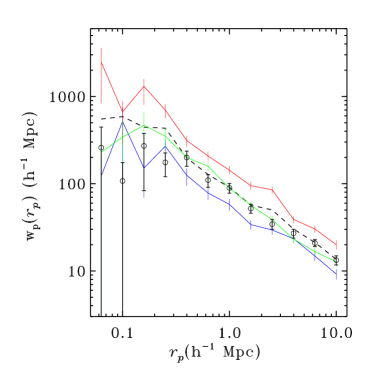
Figure 11: The projected cross-correlation function between red and blue sequence galaxies $w_{p}^{r,b}(r_{p})$ are shown as open circles. The solid lines are the auto-correlation function of the red and blue galaxies. The dashed line is the red-blue geometric mean $w_{p}^{\overline{r,b}}(r_{p})$. On scales larger than $\sim 3h^{-1}{\rm\,Mpc}$, the cross-correlation approaches the geometric mean. For scales $0.2h^{-1}{\rm\,Mpc}<r_{p}<2h^{-1}{\rm\,Mpc}$, the cross-correlation function is systematically below the geometric mean. This result suggests that on small scales, blue and red galaxies are spatially segregated beyond what was expected from their auto-correlation function. This is consistent with the morphology density relation (Dressler, 1980).

As discussed in section 3.1.2, one way to understand the relationship between two populations is to compare the projected cross-correlation function between the two with their geometric mean. If the two populations are mixed evenly, the cross-correlation functions should trace the geometric mean. If they are spatial segregated (partially) beyond what was expected from their respective auto-correlation function, the cross-correlation function should be systematically below the geometric mean. The projected cross-correlation functions for the red and blue galaxies $w_{p}^{r,b}(r_{p})$ are plotted as open circles in Figure 11. Also plotted for comparison are the red and blue auto-correlation functions (solid lines), and the red-blue geometric mean $w_{p}^{\overline{r,b}}(r_{p})$ (dashed lines). On scales larger than $\sim 3h^{-1}{\rm\,Mpc}$, the $w_{p}^{r,g}(r_{p})$ approaches the geometric mean. For scales $0.2<r_{p}<2h^{-1}{\rm\,Mpc}$, $w_{p}^{r,g}(r_{p})$ is systematically below the geometric mean for the full distribution (left panel). For the dust-corrected distribution (right panel), $w_{p}^{r,b}(r_{p})$ starts to inch below the geometric mean only from $r_{p}\lesssim 0.7h^{-1}{\rm\,Mpc}$ onwards. Our results are consistent with the partial morphology segregation within galaxy clusters (Dressler, 1980). At the one-halo regime ($r_{p}\lesssim 1-3h^{-1}{\rm\,Mpc}$), the relevant scales for galaxy clusters, red galaxies tend to occupy the cores of the clusters, while blue galaxies tend to lie towards the periphery. The lower level of spatial mixing on these scales suppresses amplitude of the cross-correlation function. Note that the green auto-correlation function (green solid line) does trace the red-blue geometric mean on large scales, suggesting that blue and red galaxies do mix evenly on these scales.

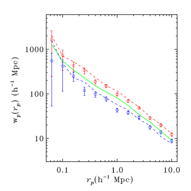
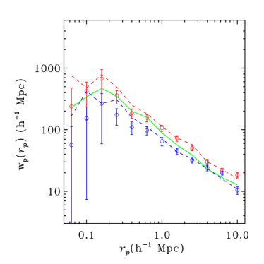
Figure 12: The projected cross-correlation function of green sample with blue $w_{p}^{g,b}(r_{p})$ (blue open circles) and red $w_{p}^{g,r})(r_{P})$ (red open circles) subsamples. The solid line shows the auto-correlation function of the green sample. The dashed lines are the geometric mean of the green-red (in red) and green-blue (in blue) auto-correlation. On the left (right) we show the analysis from the full (dust-corrected) distribution from the volume-limited sample. (See Figure 13 for more details.)

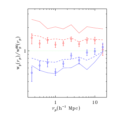
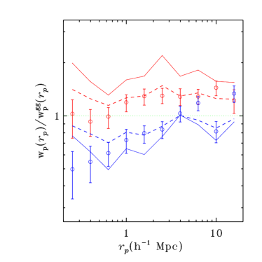
Figure 13: The ratio of projected correlation function ($w_{p}(r_{p})$) with the auto-correlation function ($w_{p}^{gg}(r_{p})$) of the green subsample. The two ratios from the cross-correlation functions, $w_{p}^{g,r}(r_{p})$ and $w_{p}^{g,b}(r_{p})$, are indicated by colored open circles. Dashed lines are for geometric means, as in figure 12. The additional solid lines are ratios from the auto-correlation function of red and blue respectively. The fact that both $w_{p}^{g,r}(r_{p})$ and $w_{p}^{g,b}(r_{p})$ are below their respective geometric mean on small scales suggest that both red and blue galaxies are found in different environments compared to the green on these scales, albeit with large uncertainties.

Figure 12 shows the projected cross-correlation function between the green and red $w_{p}^{g,r}(r_{p})$, and green and blue $w_{p}^{g,b}(r_{p})$. The solid green line is the auto-correlation function of the green sample ($w_{p}^{gg}(r_{p})$), while the dashed lines are the geometric means: $w_{p}^{\overline{g,r}}(r_{p})$ and $w_{p}^{\overline{g,b}}(r_{p})$. For the full distribution (left panel), $w_{p}^{g,r}(r_{p})$ is systematically below $w_{p}^{\overline{g,r}}$ for a range of scales within errors. $w_{p}^{g,b}(r_{p})$ are consistent, or slightly above $w_{p}^{\overline{g,b}}(r_{p})$ for $r_{p}\gtrsim 1h^{-1}{\rm\,Mpc}$, and systematically below for $0.3\lesssim r_{p}\lesssim 1h^{-1}{\rm\,Mpc}$. These inferences are shown more clearly in Figure 13 (left for full, right for dust-corrected), where we plot the normalized cross clustering strength – the ratio $w_{p}^{g,x}/w_{p}^{gg}$, where $x$ is either red, or blue – relative to the auto-correlation of the green galaxies. The additional solid lines are the normalized ACF of the red and blue. This suggest that red and green are consistent with being drawn from the same statistical sample on average for a large range of scales with a slight anti-bias on small scales. For the green and blue, there is a stronger anti-bias for $r\lesssim 1h^{-1}{\rm\,Mpc}$ as they avoid each other on these scales. Our results suggest that on scales typical of dark matter halos, galaxies drawn from the green and blue populations are less associated than would be predicted by their respective auto-correlation function.

5 Discussion

5.1 Comparison with DEEP2 $z\sim 1$

The GALEX $NUV$ selected sample used in our analysis is directly comparable to the high redshift ($z\approx 1$) galaxy sample of the DEEP2 survey (Coil et al., 2008) since their optical selection mimics the rest-frame $NUV$. In that paper, clustering analysis was done on green valley galaxies for the first time. In their analysis, the green valley $\xi(r_{p},\pi)$ appears to display kinematic structure intermediate between red and blue galaxies, with an intermediate finger-of-God effect and an intermediate overall clustering amplitude. When redshift space distortion is removed, the projected correlation function $w_{p}(r_{p})$ shows a scale dependence convergence. At $r_{p}>1h^{-1}{\rm\,Mpc}$ the functions converge to those of red populations, while for $r_{p}<1h^{-1}{\rm\,Mpc}$ it tends toward the clustering of the blue population.

In contrast, we find that our green valley $\xi(r_{p},\pi)$ has a strong finger-of-God effect consistent with that measured for red sequence galaxies, differing only in their amplitude. This can be seen most clearly in the $w_{p}(r_{p})$ analysis for the volume-limited sample (Figure 6), where the green function has form similar to that of the red function for scales $0.2<r_{p}<15h^{-1}{\rm\,Mpc}$, but is displaced to lower amplitude. It is noteworthy that the slope of the blue correlation function begins shallowing at $r\sim 1h^{-1}{\rm\,Mpc}$, displaying the kind of one-halo and two-halo segregation expected from a correlation function dominated by central galaxies. In contrast to Coil et al. (2008), the green auto-correlation function converges to that of the blue at $r_{p}>1h^{-1}{\rm\,Mpc}$. We emphasize that the green galaxy sample of Coil et al. (2008) is defined differently from ours. We divide the CMD into three disjoint parts to separate our galaxies into the subpopulations while in Coil et al., the green overlaps both the red and the blue.

5.2 Green Valley

Many recent studies reveal that blue sequence mass has remained roughly constant since $z\sim 1$ (Blanton, 2006; Faber et al., 2007) because the average ongoing star formation over $0<z\lesssim 1$ is balanced by mass flux off the blue sequence, presumably towards the build-up of the red sequence since $z\approx 1$ (Bell et al., 2004; Martin et al., 2007). Hence, green valley galaxies occupy a position where one expect to find many transitional galaxies. Martin et al. also note that the AGN fraction peaks at the green valley. For our green valley definition using the oblique color cuts from Figure 1, the AGN fraction is $\sim 50\%$.

In their study of AGN using SDSS, Constantin & Vogeley (2006) found that the redshift space two-point correlation function of Seyferts is less clustered than that of LINERS (low-ionization nuclear emission-line regions). However, Miller et al. (2003) and Li et al. (2006b) found that AGN as a whole cluster similarly as typical $L^{*}$ galaxies, if one takes into account luminosity bias. Wang & Kauffmann (2008) argues that almost all galaxies in the local universe with stellar mass $\gtrsim 10h^{-1}{\rm\,M_{\sun}}$ have active nuclei, often LINERS with lines too weak to be detected spectroscopically in SDSS. Our green galaxies, with luminosities peaked at $M_{r}\sim-21$, have stellar masses well above $10h^{-1}{\rm\,M_{\sun}}$, and could be dominated by LINERS (either detected or undetected). This would in part explain the clustering effect we see in Figures 3 and 4 (middle panels) where those bulge-dominated LINERS display kinematics similar to red sequence (primarily non-active) galaxies. The reason that AGN from $r$-band selected survey (e.g. Miller et al., 2003) cluster on average much like typical $L^{*}$ galaxies may merely be coincidental.

The lack of such behavior in the $z\sim 1$ green valley (Coil et al., 2008) may be attributable to evolution in the AGN population. There may be fewer LINERS, or the red sequence galaxies may have been experiencing more gas infall, feeding their AGN. We note that with a relative bias $\sim 1.1$, green galaxies cluster similarly to a typical galaxy with $L^{*}-0.5\approx-21$, the median luminosity of our sample.

As was discussed in section 4.1, a substantial fraction of the galaxies in the green valley are dusty star forming galaxies. Because dust content can modify the color-magnitude diagram we use to separate the galaxies into red, green and blue populations, this might potentially change the behavior of the correlation function. We argue here that to the extent that dust modifies the number counts of green galaxies, it is to promote the migration from the blue sequence to the green valley (Choi et al., 2007). Our results from Figure 4 (for the volume-limited sample) suggest that their influence in modest at best, and merely acts as additional poisson noise to the two-dimensional $\xi(\pi,r_{p})$ without altering the kinematics in the sample. The projected correlation functions of Figure 6 show similar characteristics.

5.3 Blue ($UV$) vs. Blue ($\rm Optical$)

In their studies using $g-r$ color, Zehavi et al. (2005) found that the correlation function of blue galaxies exhibits a lower amplitude and shallower correlation functions. By fitting the $w_{p}(r_{p})$ with halo occupation distribution (HOD) models, they found that the majority ($\sim 70-90$%) of blue galaxies are central galaxies in dark matter halos, usually halos with mass $\lesssim 10^{13}M_{\sun}$, in contrast to only the most luminous red galaxies being central objects of massive halos, while the majority of (less luminous) red galaxies are satellites. This fits well with the notion that blue galaxies are field galaxies – the central objects of low mass halos; red galaxies, with the exception of the central galaxy in clusters and groups, are mostly satellites of massive halos.

One can infer a similar conclusion from the auto-correlation $w_{p}(r_{p})$ plot for the blue galaxies (Figure 6). If we decompose the correlation function into two parts, one due to the one halo term and the other due to the two halo term, blue galaxies show strong two-halo excess on scales $\gtrsim 1h^{-1}{\rm\,Mpc}$, implying that on those such scales, the majority of galaxy pairs are from different halos. This was seen in the optical analysis of Zehavi et al. (2005) but prominently in our blue sequence sample. For the dust-corrected volume-limited sample (right panel of Figure 6), the amplitude of the auto-correlation function of the blue sample beyond $\sim 3h^{-1}{\rm\,Mpc}$ actually rises to match the clustering strength of the green sample.

Li et al. (2006a) found that the dependence of $w_{p}(r_{p})$ on optical $g-r$ color extends beyond $5h^{-1}{\rm\,Mpc}$, suggesting that the conventional wisdom that clustering should converge at large scales may not occur until at a scales larger than $5h^{-1}{\rm\,Mpc}$. Here, we argue that this is an effect due to the mixture of population between blue galaxies, and green and red; that the optical $g-r$ color does not have sufficient power to separate the green from the blue. Blue galaxies, by themselves, have a very pronounced two halo excess and are dominated entirely by central galaxies, flattening the correlation function substantially at large scales, compared to the red and green population. To the extent that one can eliminate or correct for the internal reddening due to dust, $NUV-r$ color is very efficient in isolating a sequence of purely star-forming galaxies.

6 Summary and Conclusions

We have constructed a GALEX and SDSS matched catalog, where we have used the GR3 catalog from GALEX and the SDSS DR5 main spectroscopic galaxy sample. We construct the galaxy distribution of $NUV-r$ vs $M_{r}$ color-magnitude diagram, and divide the distribution into populations of red sequence, green valley and blue sequence. Since our main goal is to study the color dependence of clustering, we took substantial care in matching the luminosity distribution of each population. For each population, we measure the two-dimensional correlation function $\xi(\pi,r_{p})$, and the one-dimensional projected correlation function $w_{p}$. We also perform cross-correlation analyses between each of the sub-populations.

Our principle finding is that the red sequence and green valley appear to show similar clustering properties, as expressed in the finger-of-God effect in the auto-correlation function. The projected correlation function is consistent with red and green galaxies residing as satellites of massive halos, while the blue sequence shows what appears to be a clear two-halo signature, hence primarily serving as central galaxies of less massive halos. The cross-correlation function also shows that green and blue galaxies, on small scales, are not a mere statistical mix, but are spatially segregated from each other.

The findings would appear to place the green valley population with the red sequence. The green valley would largely consist of massive galaxies that reside in massive halos, and which cluster like the red sequence. We note that Martin et al. (2007), Wyder et al. (2007), and Salim et al. (2007) show that a large fraction of type II AGN are found in the green valley. Salim et al. show that in the plot of specific star formation rate vs stellar mass, the AGN tend to be found in massive ($>3\times 10^{10}M_{\odot}$) galaxies. The AGN occupy a region in these plots that strongly resembles that of the reddest class of galaxies, the “no-H$\alpha$” red sequence galaxies. Significantly, the AGN are clearly offset from the locus of the blue sequence, in the plot of specific star-formation rate (SFR) versus mass. The significance is that while a minority of AGN are found with properties that coincide with those of the more massive blue sequence galaxies, green valley galaxies – the subsample with the largest AGN fraction — exhibit properties similar to those of the red sequence, but showing mildly elevated star formation.

In this study, we have shown that the green valley population clusters in ways that are characteristic of, but also less strongly than, the red sequence. One may suggest that these studies paint a picture in which both the properties of the green valley and the “demographics” are different from those of the blue sequence, at the present epoch. These findings do not necessarily contradict the studies that find an increase in the total mass of red sequence galaxies since $z\sim 1$. They do suggest, however, that if blue sequence galaxies evolve by some process to the green valley, and ultimately to the red sequence, such evolution must also accompanied by a transition from the field environment to a group/cluster environment. Such a change could conceivably occur if the blue population resides along filaments that infall into clusters, over time. Our cross-correlation results show that green galaxies avoid both red and blue galaxies on small scales is consistent with the change in environment hypothesis. We note that models like ram pressure stripping (Gunn & Gott, 1972), starvation of (cold) gas, and the virial shock heating model of (Dekel & Birnboim, 2006) naturally incorporate environmental factors in their mechanism for color transformation in galaxies.

It is also possible that the downsizing (Cowie et al., 1996) effect is so strong that most star forming galaxies are evolving rapidly with redshift (e.g. Tinsley, 1968). One must recall that star forming activity at $z\sim 1$ resides in considerably more massive galaxies, and that a color-based population separation, as we have done, will refer to much higher masses; the rest-frame colors may be similar, but the fundamental nature of the galaxies, not.

One may speculate that the the green valley is occupied by nominally red galaxies that experience the infall of a gas rich system that either induces star formation and/or fuels the AGN, rendering it visible via its emission lines. However, the feedback of an AGN might inhibit star formation and move a blue sequence galaxy to the green valley. Any number of environmental effects (e.g. harassment, starvation) might speed the consumption of gas in a disk, again moving a galaxy to the green valley. A small sample of optically quiescent members of the green valley that nominally have a UV excess show clear star formation signatures (spirals) when imaged in the UV using HST (Salim & Rich, 2009). There is still the issue of the origin of the low mass red sequence, and the evolution of blue sequence, into the green valley and ultimately the red sequence, might have an important role in the growth of the lower mass portion of the red sequence. This was partially addressed by semi-analytical work of Benson et al. (2003) and Bower et al. (2006).

In contrast to the construction of color-magnitude diagrams for stellar populations, the environment, for galaxies, is a critical physical variable in their evolution. This is true both the in the sense of their dark matter environment as well as the presence of detectable companion stellar systems. In considering the major processes driving galaxy evolution, it would appear that evolution of both of these observables must be considered, as a function of look-back time.

References

- Basu-Zych et al. (2008) Basu-Zych, A.R., et al., 2008, submitted to ApJ
- Bell et al. (2004) Bell, E.F., et al., 2004, ApJ, 608, 752
- Benson et al. (2003) Benson, A.J., et al., 2003, ApJ, 599, 38
- Bertin & Arnouts (1996) Bertin, E., & Arnouts, S., 1996, A&AS, 117, 393
- Blanton (2000) Blanton, M.R., 2000, ApJ, 544, 63
- Blanton et al. (2003) Blanton, M.R., et al., 2003, ApJ, 592, 819
- Blanton et al. (2005a) Blanton, M.R., et al., 2005, AJ, 129, 2562
- Blanton et al. (2005b) Blanton, M.R., et al., 2005, ApJ, 629, 143
- Blanton (2006) Blanton, M.R., 2006, ApJ, 648, 268
- Blanton & Roweis (2007) Blanton, M.R., & Roweis, S., 2007, AJ, 133, 734
- Bower et al. (1992) Bower, R.G., et al., 1992, MNRAS, 254, 601
- Bower et al. (2006) Bower, R.G., et al., 2006, MNRAS, 370, 645
- Brown et al. (2008) Brown, M.J.I., et al., 2008, ApJ, 682, 937
- Budavari et al. (2003) Budavari, T., et al., 2003, ApJ, 595, 59
- Chen (2009) Chen, J., 2009, A&A, 494, 867
- Choi et al. (2007) Choi, Y.-Y., et al., 2007, 658, 884
- Coil et al. (2008) Coil, A.L., et al., 2008, ApJ, 672, 153
- Constantin & Vogeley (2006) Constantin, A., & Vogeley, M.S., 2006, ApJ, 650, 727
- Cowie et al. (1996) Cowie, L.L, et al., 1996, AJ, 112, 839
- Croton et al. (2006) Croton, D.J., et al., 2006, MNRAS, 365, 11
- Davis & Geller (1976) Davis, M., & Geller, M.J., 1976, ApJ, 208, 13
- Davis & Peebles (1983) Davis, M., & Peebles, P.J.E., 1983, ApJ, 267, 465
- Davison & Hinkley (1997) Davison, A.C., & Hinkley, D.V., 1997, Bootstrap Methods and Their Applications (Cambridge: Cambridge Univ. Press)
- Dekel & Birnboim (2006) Dekel, A., & Birnboim, Y., 2006, MNRAS, 368, 2
- Dressler (1980) Dressler, A., 1980, ApJ, 236, 351
- Efron (1981) Efron, B., 1981, Biometrika, 68, 589
- Efstathiou et al. (1991) Efstathiou, G., et al., 1991, ApJ, 380L, 47
- Faber et al. (2007) Faber, S.M., et al., 2007, ApJ, 665, 265
- Gunn & Gott (1972) Gunn, J.E., & Gott, J.R., 1972, ApJ, 176, 1
- Heinis et al. (2007) Heinis, S., et al., 2007, ApJS, 173, 503
- Heinis et al. (2009) Heinis, S., et al., 2009, submitted to ApJ
- Haiman & Hui (2001) Haiman, Z., & Hui, L., 2001, ApJ, 547, 27
- Hamilton (1992) Hamilton, A.J.S., 1992, ApJ, 385, L5
- Hamilton & Tegmark (2002) Hamilton, A.J.S., & Tegmark, M., 2002, MNRAS, 330, 506
- Hopkins et al. (2006) Hopkins, P.F., et al., 2007, ApJS, 163, 1
- Hopkins et al. (2007) Hopkins, P.F., et al., 2007, ApJ, 659, 976
- Hubble (1936) Hubble E.P, et al., 1936, The Realm of the Nebulae (Oxford: Oxford Univ. Press), 79
- Johnson et al. (2006) Johnson, B.D., et al., 2006, ApJ, 619, L109
- Kauffmann et al. (2004) Kauffmann, G. et al., 2004, MNRAS, 341, 33
- Kaiser (1987) Kaiser, N., 1987, MNRAS, 227, 1
- Kerscher et al. (2000) Kerscher, M., et al., 2000, ApJ, 535, L5
- Kron (1980) Kron, R. G. 1980, ApJS, 43, 305
- Landy & Szalay (1993) Landy, S.D., & Szalay, A., 1993, ApJ, 412, 64
- Li et al. (2006a) Li, C., et al., 2006a, MNRAS, 368, 21
- Li et al. (2006b) Li, C., et al., 2006b, MNRAS, 373, 457
- Loh (2008) Loh, J.M., 2008, ApJ, 681, 726
- Madgwick et al. (2003) Madgwick, D.S., et al., 2003, MNRAS, 344, 847
- Martin et al. (2005) Martin, D.C., et al., 2005, ApJ, 619, L1
- Martin et al. (2007) Martin, D.C., et al., 2007, ApJS, 173, 342
- Martini & Weinberg (2001) Martini, P, & Weinberg, D.H., 2001, ApJ, 547, 12
- Miller et al. (2003) Miller, C.J., et al., 2003, ApJ, 597, 142
- Milliard et al. (2007) Milliard, B., et al., 2007, ApJS, 173,
- Morrissey et al. (2005) Morrissey, P., et al., 2005, 619, L7
- Morrissey et al. (2007) Morrissey, P., et al., 2007, ApJS, 173, 682
- Norberg et al. (2002) Norberg, P., et al., 2002, MNRAS, 332, 837
- Norberg et al. (2009) Norberg, P., et al., 2009, arXiv:0810.1885v1
- Ostriker & Steinhardt (1995) Ostriker, J.P., & Steinhardt, P.J., 1995, Nature, 377, 600
- Padmanabhan et al. (2008) Padmanabhan, N., et al., 2008, arXiv:0802.2105
- Park et al. (2007) Park, C., et al., 2007, ApJ, 658, 898
- Peebles (1980) Peebles, P.J.E., 1980, The Large-scale Structure of the Universe, Princeton Univ. Press
- Perlmutter et al. (1999) Perlmutter, S., et al., 1999, ApJ, 517, 565
- Rich et al. (2005) Rich, R.M., et al., 2005, ApJ, 619L, 107
- Salim & Rich (2009) Salim, S., & Rich, R.M., 2009, BAAS 213, 435.03
- Riess et al. (1998) Riess, A.G., et al., 1998, AJ, 116, 1009
- Salim et al. (2007) Salim, S., et al., 2007, ApJS, 173, 267
- Sargent & Turner (1977) Sargent, W.L.W., & Turner, E.L., 1977, ApJ, 212, L3
- Seljak & Warren (2004) Seljak, U., & Warren, M.S., 2004, MNRAS, 355, 129
- Schiminovich et al. (2007) Schinomovich, D., et al., 2007, ApJS, 173, 315
- Silk & Rees (1998) Silk, J., & Rees, M.J., 1998, A&A, 331L, 1
- Swanson et al. (2008) Swanson, M.E.C., et al., (2008), MNRAS, 387, 1391
- Spergel et al. (2007) Spergel, D.N., et al., 2007, ApJS, 170, 377
- Tinker (2007) Tinker, J., 2007, MNRAS, 374, 477
- Tinsley (1968) Tinsley, B.M., 1968, ApJ, 151, 547
- Toomre & Toomre (1972) Toomre, A., & Toomre, J., 1972, ApJ, 178, 623
- Totsuji & Kihara (1969) Totsuji, H., & Kihara, T., 1969, PASJ, 21, 221
- Wang & Kauffmann (2008) Wang, L., & Kauffmann, G., 2008, MNRAS, 391 785
- Wang et al. (2007) Wang, Y., et al., 2007, ApJ, 664, 609
- Wyder et al. (2007) Wyder, T. K., et al.2007, ApJS, 173, 293
- York et al. (2000) York D. et al., 2000, AJ, 120, 1579
- Zehavi et al. (2005) Zehavi, I., et al., 2005, ApJ, 630, 1
- Zwicky et al. (1968) Zwicky, F., et al., 1968, Catalog of Galaxies and of Clusters of Galaxies, Vols. 1 – 6 (Pasadena, Caltech)