Optimally (Distributional-)Robust Kalman Filtering

Abstract

We present optimality results for robust Kalman filtering where robustness is understood in a distributional sense, i.e.; we enlarge the distribution assumptions made in the ideal model by suitable neighborhoods. This allows for outliers which in our context may be system-endogenous or -exogenous, which induces the somewhat conflicting goals of tracking and attenuation.

The corresponding minimax MSE-problems are solved for both types of outliers separately, resulting in closed-form saddle-points which consist of an optimally-robust procedure and a corresponding least favorable outlier situation. The results are valid in a surprisingly general setup of state space models, which is not limited to a Euclidean or time-discrete framework.

The solution however involves computation of conditional means in the ideal model, which may pose computational problems. In the particular situation that the ideal conditional mean is linear in the observation innovation, we come up with a straight-forward Huberization, the rLS filter, which is very easy to compute. For this linearity we obtain an again surprising characterization.

label=e1]Peter.Ruckdeschel@itwm.fraunhofer.de

1 Introduction

Robustness issues in Kalman filtering have long been a research topic, with first (non-verified) hits on a quick search for “robust Kalman filter” on scholar.google.com as early as 1962 and 1967, i.e.; the former even before the seminal Huber (1964) paper, often referred to as birthday of Robust Statistics.

In the meantime there is an ever growing amount of literature on this topic —Kassam and Poor (1985) have already compiled as many as 209 references to that subject in 1985. Excellent surveys are given in, e.g. Kassam and Poor (1985), Stockinger and Dutter (1987), Schick and Mitter (1994), Künsch (2001).

In these references you find many different notions of robustness, all somewhat related to stability but measuring this stability w.r.t. deviations of various “input parameters”; in this paper we are concerned with (distributional) minimax robustness; i.e.; we work with suitable distributional neighborhoods about an ideal model, already used by Birmiwal and Shen (1993) and Birmiwal and Papantoni-Kazakos (1994), and then solve the problem to find the procedure minimizing the maximal predictive inaccuracy on these neighborhoods—measured in terms of mean squared error (MSE)—in quite generality, compare Theorems 3.2, 3.10, 4.1. In the particular situation that the ideal conditional mean is linear in the observation innovation (for a definition see subsection 2.3.2), the minimax filter is a straight-forward Huberization, the rLS filter, which is extremely easy to compute. For this linearity we obtain a surprising characterization in Propositions 3.4 and 3.6. This motivates a corresponding optimal test for linearity, Proposition 3.8. Even in situations where no or only partial knowledge of the size of the contamination is available we can distinguish an optimal procedure, compare Lemma 3.1.

2 General setup

2.1 Ideal model

In this section, we start with some definitions and assumptions. We are working in the context of state space models (SSM’s) as to be found in many textbooks, cf. e.g. Anderson and Moore (1979), Harvey (1991), and Durbin and Koopman (2001).

2.1.1 Time Discrete, linear Euclidean Setup

The most prominent setting in this context is the linear, time–discrete, Euclidean setup, which will serve as reference setting in this paper: An unobservable $p$-dimensional state $X_{t}$ evolves according to a possibly time-inhomogeneous vector autoregressive model of order $1$ (VAR(1)) with innovations $v_{t}$ and transition matrices $F_{t}$, i.e.,

$$X_{t}=F_{t}X_{t-1}+v_{t}$$ (2.1)

The statistician observes a $q$-dimensional linear transformation $Y_{t}$ of $X_{t}$ and in this makes an additive observation error $\varepsilon_{t}$,

$$Y_{t}=Z_{t}X_{t}+\varepsilon_{t}$$ (2.2)

In the ideal model we work in a Gaussian context, that is we assume

$$v_{t}\sim{\cal N}_{p}(0,Q_{t}),\qquad\varepsilon_{t}\sim{\cal N}_{q}(0,V_{t}),\qquad X_{0}\sim{\cal N}_{p}(a_{0},Q_{0}),$$ (2.3)

$${X_{0},v_{s},\varepsilon_{t},\;s,t\in\mathbb{N}\;\;\mbox{ stochastically independent}}$$ (2.4)

As usual, normality assumptions may be relaxed to working only with specified first and second moments, if we restrict ourselves to linear unbiased procedures as in the Gauss-Markov setting.
For this paper, we assume the hyper–parameters $F_{t},Z_{t},Q_{t},V_{t},a_{0}$ to be known.

2.1.2 Generalizations covered by the present approach

Parts of our results (more specifically, all of sections 3.2, 3.4) also cover much more general SSMs; in this paragraph we sketch some of these. To begin with, as long as MSE makes sense for the range of the states, these results cover general Hidden Markov Models for arbitrary observation space as given by

$$P(X_{0}\in A)=\int_{A}p_{0}^{X_{0}}(x)\,\mu_{0}(dx)$$ (2.5)

$$P(X_{t}\in A|X_{t-1}=x_{t-1},\ldots,X_{0}=x_{0})=\int_{A}p_{t}^{X_{t}|X_{t-1}=x_{t-1}}(x)\,\mu_{t}(dx),$$ (2.6)

$$P(Y_{t}\in B|X_{t}=x_{t})=\int_{B}q_{t}^{Y_{t}|X_{t}=x_{t}}(y)\,\nu_{t}(dy)$$ (2.7)

In this setting, we assume known (and existing) [regular conditional] densities $p_{0}^{X_{0}}$, $p_{t}^{\,\cdot\,|\,\cdot\,}$, $q_{t}^{\,\cdot\,|\,\cdot\,}$ w.r.t. known measures $\nu_{t}$, $\mu_{t}$ on $\mathbb{B}^{q}$ and $\mathbb{B}^{p}$, respectively. Dynamic (generalized) linear models as discussed in West et al. (1985) and West and Harrison (1989) are covered as well —under corresponding assumptions as to (conditional) densities and range of the states. In applications of Mathematical Finance we also need to cover continuous time settings, i.e.; there is an unobservable state evolving according to an SDE

$$dX_{t}=f(t,X_{t})\,dt+q(t,X_{t})\,dW_{t}$$ (2.8)

where for $X_{0}$ we assume (2.5), while $W_{t}$, is a Wiener process, and $f$ and $q$ are suitably measurable, known functions, and observations $Y_{t}$ are either formulated as a time-continuous observation process (as in Tang (1998)) or—more often—at discrete, but not necessarily equally spaced times, compare, e.g. Nielsen et al. (2000) and Singer (2002). In this context, but also for corresponding non-linear time-discrete SSMs, a straightforward approach linearizes the corresponding transition and observation functions to give the (continuous-discrete) Extended Kalman Filter (EKF) After this linearization we are again in the context of a (time-inhomogeneous) linear SSM, hence the methodology we develop in the sequel applies to this setting as well.

So far we do not cover approaches to improve on this simple linearization, notably the second order nonlinear filter (SNF) introduced in Jazwinski (1970), also cf. Singer (2002, sec. 4.3.1). the unscented Kalman filter (UKF) (Julier et al., 2000) and Hermite expansions as in Aït-Sahalia (2002), see also Singer (2002, sec. 4.3).

Going one more step ahead, to cover applications such as portfolio optimization, we may allow for controls $U_{t}$ to be set or determined by the statistician, and which are fed back in the state equations. In the context of the continuous time model, this is also known as SDEX, cf. Nielsen et al. (2000), and for the application of stochastic control to portfolio optimization, cf. Korn (1997). In this setting, controls $U_{t}$ are usually assumed measurable w.r.t.  $\sigma(Y_{t-})$; to integrate them into our setting, we simply have to integrate them in the corresponding condition vectors.

Finally, the question of specifying the order of conditioning left aside, we do not make use of the linearity of time, so our minimax results also cover suitable formulations of indirectly observed random fields.

2.2 Deviations from the ideal model

As usual with Robust Statistics, the ideal model assumptions we have specified so far are extended by allowing (small) deviations, most prominently generated by outliers. In our notation, suffix “${\textstyle\rm id}$” indicates the ideal setting, “${\textstyle\rm di}$” the distorting (contaminating) situation, “${\textstyle\rm re}$” the realistic, contaminated situation.

2.2.1 AO’s and IO’s

In SSM context (and contrary to the independent setting), outliers may or may not propagate. Following the terminology of Fox (1972), we distinguish innovation outliers (or IO’s) and additive outliers (or AO’s). Historically, AO’s denote gross errors affecting the observation errors, i.e.,

$${\rm AO} :: \varepsilon^{\scriptscriptstyle\rm re}_{t}\sim(1-r_{\scriptscriptstyle\rm AO}){\cal L}(\varepsilon^{\scriptscriptstyle\rm id}_{t})+r_{\scriptscriptstyle\rm AO}{\cal L}(\varepsilon^{\scriptscriptstyle\rm di}_{t})$$ (2.9)

where ${\cal L}(\varepsilon^{\scriptscriptstyle\rm di}_{t})$ is arbitrary, unknown and uncontrollable (a.u.u.) and $0\leq r_{\scriptscriptstyle\rm AO}\leq 1$ is the AO-contamination radius, i.e.; the probability for an AO. IO’s on the other hand are usually defined as outliers which affect the innovations,

$${\rm IO} :: v^{\scriptscriptstyle\rm re}_{t}\sim(1-r_{\scriptscriptstyle\rm IO}){\cal L}(v^{\scriptscriptstyle\rm id}_{t})+r_{\scriptscriptstyle\rm IO}{\cal L}(v^{\scriptscriptstyle\rm di}_{t})$$ (2.10)

where again ${\cal L}(v^{\scriptscriptstyle\rm di}_{t})$ is a.u.u. and $0\leq r_{\scriptscriptstyle\rm IO}\leq 1$ is the corresponding radius.

We stick to this distinction for consistency with literature, although we rather use these terms in a wider sense, unless explicitly otherwise stated: IO’s denote endogenous outliers affecting the state equation in general, hence distortion propagates into subsequent states. This also covers level shifts or linear trends; which if $|F_{t}|<1$ are not included in (2.10), as IO’s would then decay geometrically in $t$. We also extend the meaning of AO’s to denote general exogenous outliers which enter the observation equation only and thus do not propagate, like substitutive outliers or SO’s defined as

$${\rm SO} :: Y^{\scriptscriptstyle\rm re}_{t}\sim(1-r_{\scriptscriptstyle\rm SO}){\cal L}(Y^{\scriptscriptstyle\rm id}_{t})+r_{\scriptscriptstyle\rm SO}{\cal L}(Y^{\scriptscriptstyle\rm di}_{t})$$ (2.11)

where again ${\cal L}(Y^{\scriptscriptstyle\rm di}_{t})$ is a.u.u.  and $0\leq r_{\scriptscriptstyle\rm SO}\leq 1$ is the corresponding radius.

Apparently, the SO-ball of radius $r$ consisting of all ${\cal L}(Y^{\scriptscriptstyle\rm re}_{t})$ according to (2.11) contains the corresponding AO-ball of the same radius when $Y^{\scriptscriptstyle\rm re}_{t}=Z_{t}X_{t}+\varepsilon^{\scriptscriptstyle\rm re}_{t}$. However, for technical reasons, we make the additional assumption that

$$Y^{\scriptscriptstyle\rm id}_{t},Y^{\scriptscriptstyle\rm di}_{t}\quad\mbox{stochastically independent}$$ (2.12)

and then this relation no longer holds.

2.2.2 Different and competing goals induced by endogenous and exogenous outliers

In the presence of AO’s we would like to attenuate their effect, while when there are IO’s, the usual goal in online applications would be tracking, i.e.; detect structural changes as fast as possible and/or react on the changed situation. A situation where both AO’s and IO’s may occur poses an identification problem: Immediately after a suspicious observation we cannot tell IO type from AO type. Hence a simultaneous treatment of both types will only be possible with a certain delay—see Ruckdeschel (2010).

2.3 Classical Method: Kalman–Filter

2.3.1 Filter Problem

The most important problem in SSM formulation is to reconstruct the unobservable states $X_{t}$ based on the observations $Y_{t}$. For abbreviation let us denote

$$Y_{1:t}=(Y_{1},\ldots,Y_{t}),\quad Y_{1:0}:=\emptyset$$ (2.13)

Then using MSE risk, the optimal reconstruction is distinguished as

$$\mathop{\rm{{}E{}}}\nolimits\big{|}X_{t}-f_{t}\big{|}^{2}=\min\nolimits_{f_{t}},\qquad f_{t}\mbox{ measurable w.r.t.\ }\sigma(Y_{1:s})$$ (2.14)

Depending on $s$ this is a prediction ($s<t$), a filtering ($s=t$) and a smoothing problem ($s>t$). In the sequel we will confine ourselves to the filtering problem.

2.3.2 Kalman–Filter

It is well-known that the general solution to (2.14) is the corresponding conditional expectation $\mathop{\rm{{}E{}}}\nolimits[X_{t}|Y_{1:s}]$. Except for the Gaussian case, this exact conditional expectation may be computational too expensive. Hence similar to the Gauss-Markov setting, it is common to restrict oneself to linear filters. In this context, the seminal work of Kalman (1960) (discrete-time setting) and Kalman and Bucy (1961) (continuous-time setting) introduced effective schemes to compute this optimal linear filter $X_{t|t}$. In discrete time, we reproduce it here for later reference:

Init.: $$X_{0|0} =a_{0},\qquad \Sigma_{0|0} =Q_{0}$$ (2.15)

Pred.: $$X_{t|t-1} =F_{t}X_{t-1|t-1},\qquad \Sigma_{t|t-1} =F_{t}\Sigma_{t-1|t-1}F_{t}^{\tau}+Q_{t}$$ (2.16)

Corr.: $$X_{t|t} =X_{t|t-1}+M^{0}_{t}\Delta Y_{t},\!\!\!\quad \Sigma_{t|t} =({\mathbb{I}}_{p}-M^{0}_{t}Z_{t})\Sigma_{t|t-1}$$ (2.17)

for $$\Delta X_{t} =X_{t}-X_{t|t-1},\!\!\!\quad \Delta Y_{t} =Y_{t}-Z_{t}X_{t|t-1}=Z_{t}\Delta X_{t}+\varepsilon_{t},$$

$$\Delta_{t} =Z_{t}\Sigma_{t|t-1}Z_{t}^{\tau}+V_{t},\!\!\!\quad M^{0}_{t} =\Sigma_{t|t-1}Z_{t}^{\tau}\Delta_{t}^{-}$$ (2.18)

and where $\Delta X_{t}$ is the prediction error, $\Delta Y_{t}$ the observation innovation, and $\Sigma_{t|t}=\mathop{\rm Cov}\nolimits(\Delta X_{t})$, $\Sigma_{t|t-1}=\mathop{\rm Cov}\nolimits(X_{t}-X_{t|t-1})$, $\Delta_{t}=\mathop{\rm Cov}\nolimits(\Delta Y_{t})$; $M^{0}_{t}$ is the so-called Kalman gain, and $\Delta_{t}^{-}$ stands for the Moore-Penrose inverse of $\Delta_{t}$.

2.3.3 Optimality of the Kalman–Filter

Realizing that $M^{0}_{t}\Delta Y_{t}$ is an orthogonal projection, it is not hard to see that the (classical) Kalman filter solves problem (2.14) (for $s=t$) among all linear filters. Using orthogonality of $\{\Delta Y_{t}\}_{t}$ once again, we may setup similar recursions for the corresponding best linear smoother; see, e.g. Anderson and Moore (1979), Durbin and Koopman (2001). Under normality, i.e.; assuming (2.3), we even have $X_{t|t[-1]}=\mathop{\rm{{}E{}}}\nolimits[X_{t}|Y_{1:t[-1]}]$, i.e.; the Kalman filter is optimal among all $Y_{1:t[-1]}$-measurable filters. It also is the posterior mode of ${\cal L}(X_{t}|Y_{1:t})$ and $X_{t|t}$ can also be seen to be the ML estimator for a regression model with random parameter; for the last property, compare Duncan and Horn (1972).

2.3.4 Features of the Kalman–Filter

The Kalman filter stands out for its clear and understandable structure: it comes in three steps, all of which are linear, hence cheap to evaluate and easy to interpret. Due to the Markovian structure of the state equation, all information from the past useful for the future may be captured in the value of $X_{t|t-1}$, so only very limited memory is needed.
From a (distributional) Robustness point of view, this linearity at the same time is a weakness of this filter—$y$ enters unbounded into the correction step which hence is prone to outliers. A good robustification of this approach would try to retain as much as possible from these positive properties of the Kalman filter while revising the unboundedness in the correction step.

3 The rLS as optimally-robust filter

3.1 Definition

3.1.1 robustifying recursive Least Squares: rLS

In a first step we limit ourselves to AO’s. Notationally, where clear from the context, we suppress the time index $t$. As no (new) observations enter the initialization and prediction steps, these steps may be left unchanged. In the correction step, we will have to modify the orthogonal projection present in (2.17). Suggested by H. Rieder and worked out in Ruckdeschel (2001, ch. 2), the following robustification of the correction step is straightforward: Instead of $M^{0}\Delta Y$, we use a Huberization of this correction

$$H_{b}(M^{0}\Delta Y)=M^{0}\Delta Y\min\{1,b/\big{|}M^{0}\Delta Y\big{|}\}$$ (3.1)

for some suitably chosen clipping height $b$. Apparently, this proposal removes the unboundedness problem of the classical Kalman filter while still remaining reasonably simple, in particular this modification is non-iterative, hence especially useful for online-purposes.

3.1.2 Choice of the clipping height $b$

For the choice of the clipping height $b$, we have two proposals. Both are based on the simplifying assumption that $\mathop{\rm{{}E{}}}\nolimits_{\rm\scriptscriptstyle id}[\Delta X|\Delta Y]$ is linear, which will turn out to only be approximately right. The first one, an Anscombe criterion, chooses $b=b(\delta)$ such that

$$\mathop{\rm{{}E{}}}\nolimits_{\rm\scriptscriptstyle id}\big{|}\Delta X-H_{b}(M^{0}\Delta Y)\big{|}^{2}\stackrel{{\scriptstyle!}}{{=}}(1+\delta)\mathop{\rm{{}E{}}}\nolimits_{\rm\scriptscriptstyle id}\big{|}\Delta X-M^{0}\Delta Y\big{|}^{2}$$ (3.2)

$\delta$ may be interpreted as “insurance premium” to be paid in terms of loss of efficiency in the ideal model compared to the optimal procedure in this (ideal) setting, i.e.; the classical Kalman filter.

The second criterion for a given radius $r\in[0,1]$ of the (SO-) neighborhood ${\cal U}^{\rm\scriptscriptstyle SO}(r)$ determines $b=b(r)$ such that

$$(1-r)\mathop{\rm{{}E{}}}\nolimits_{\rm\scriptscriptstyle id}(|M^{0}\Delta Y|-b)_{+}\stackrel{{\scriptstyle!}}{{=}}rb$$ (3.3)

Assuming linear ideal conditional expectations, this will produce the minimax-MSE procedure for ${\cal U}^{\rm\scriptscriptstyle SO}(r)$ according to Theorem 3.2 below.

One might object that (3.3) assumes $r$ to be known, which in practice hardly ever is true. If $r$ is unknown however, we translate an idea worked out in Rieder et al. (2008): Assume we have limited knowledge about $r$, say $r\in[r_{l},r_{u}]$, $0\leq r_{l}<r_{u}\leq 1$. Then we distinguish a least favorable radius $r_{0}$ defined in the following expressions

$$r_{0} = {\rm argmin}_{s\in[r_{l},r_{u}]}\rho_{0}(s),\qquad\rho_{0}(s)=\max_{r\in[r_{l},r_{u}]}\rho(r,s),$$ (3.4)

$$\rho(r,s) = \frac{\max_{P\in{\cal U}^{\rm\scriptscriptstyle SO}(r)}{\rm MSE}_{P}\big{(}{\rm rLS}(b(s))\big{)}}{\max_{P^{\prime}\in{\cal U}^{\rm\scriptscriptstyle SO}(r)}{\rm MSE}_{P^{\prime}}\big{(}{\rm rLS}(b(r))\big{)}}$$ (3.5)

and use the corresponding $b(r_{0})$. Procedure ${\rm rLS}(b(r_{0}))$ then minimizes the maximal inefficiency $\rho_{0}(s)$ among all procedures ${\rm rLS}(b(r))$, i.e.; each rLS for some clipping height $b(r)\not=b(r_{0})$ has an inefficiency no smaller than $\rho_{0}(r_{0})$ for some $r^{\prime}\in[r_{l},r_{u}]$. Radius $r_{0}$ can be computed quite effectively by a bisection method: Let

$$A_{r} = \mathop{\rm{{}E{}}}\nolimits_{\rm\scriptscriptstyle id}\Big{[}\mathop{\rm{}tr{}}\mathop{\rm Cov}\nolimits_{\rm\scriptscriptstyle id}[\Delta X|\Delta Y^{\rm\scriptscriptstyle id}]+(|M^{0}\Delta Y^{\rm\scriptscriptstyle id}|-b(r))_{+}^{2}\Big{]}$$ (3.6)

$$B_{r} = \mathop{\rm{{}E{}}}\nolimits_{\rm\scriptscriptstyle id}\Big{[}|M^{0}\Delta Y^{\rm\scriptscriptstyle id}|^{2}-(|M^{0}\Delta Y^{\rm\scriptscriptstyle id}|-b(r))_{+}^{2}\Big{]}+b(r)^{2}$$ (3.7)

Then the following analogue to Kohl (2005, Lemma 2.2.3) holds:

Lemma 3.1.

In equations (3.4) and (3.5), let $r,s$ vary in $[r_{l},r_{u}]$ with $0\leq r_{l}<r_{u}\leq 1$. Then

$$\rho_{0}(r)=\max\{A_{r}/A_{r_{l}},B_{r}/B_{r_{u}}\}$$ (3.8)

and there exists some $\tilde{r}_{0}\in[r_{l},r_{u}]$ such that $A_{\tilde{r}_{0}}/A_{r_{l}}=B_{\tilde{r}_{0}}/B_{r_{u}}$. This $\tilde{r}_{0}$ is least favorable, i.e., $\min_{r\in[r_{l},r_{u}]}\rho_{0}(r)=\rho_{0}(\tilde{r}_{0})$. Moreover, if $r_{u}=1$, $r_{0}=r_{u}$.

In particular, the last equality shows that one should restrict $r_{u}$ to be strictly smaller than $1$ to get a sensible procedure.

3.2 (One-Step)-Optimality of the rLS

The (so-far) ad-hoc robustification proposed in the rLS filter has some remarkable optimality properties: Let us first forget about the time structure and instead consider the following simplified, but general “Bayesian” model:
We have an unobservable but interesting signal $X\sim P^{X}(dx)$, where for technical reasons we assume that in the ideal model $\mathop{\rm{{}E{}}}\nolimits|X|^{2}<\infty$. Instead of $X$ we rather observe a random variable $Y$ taking values in an arbitrary space of which we know the ideal transition probabilities; more specifically, we assume that these ideal transition probabilities for almost all $x$ have densities w.r.t. some measure $\mu$,

$$P^{Y|X=x}(dy)=\pi(y,x)\,\mu(dy)$$ (3.9)

Our approach uses MSE as accuracy criterion for the reconstruction, so is limited to ranges of $X$ where this makes sense. On the other hand it is this reduction to the “Bayesian” model which makes the generalizations sketched in section 2.1 possible. As (wide-sense) AO model, we consider an SO outlier model, i.e.;

$$Y^{\rm\scriptscriptstyle re}=(1-U)Y^{\rm\scriptscriptstyle id}+UY^{\rm\scriptscriptstyle di},\qquad U\sim{\rm Bin}(1,r)$$ (3.10)

for $U$ independent of $(X,Y^{\rm\scriptscriptstyle id})$ and $(X,Y^{\rm\scriptscriptstyle di})$ and some distorting random variable $Y^{\rm\scriptscriptstyle di}$ for which, in a slight variation of condition (2.12) we assume

$$Y^{\rm\scriptscriptstyle di},\;X\quad\mbox{stochastically independent}$$ (3.11)

and the law of which is arbitrary, unknown and uncontrollable. As a first step consider the set $\partial{\cal U}^{\rm\scriptscriptstyle SO}(r)$ defined as

$$\partial{\cal U}^{\rm\scriptscriptstyle SO}(r)=\Big{\{}{\cal L}(X,Y^{\rm\scriptscriptstyle re})\,|\,Y^{\rm\scriptscriptstyle re}\;\mbox{acc. to \eqref{YSO} and \eqref{indep2}}\Big{\}}$$ (3.12)

Because of condition (3.11), in the sequel we refer to the random variables $Y^{\rm\scriptscriptstyle re}$ and $Y^{\rm\scriptscriptstyle di}$ instead of their respective (marginal) distributions only, while in the common gross error model as present in (2.9) or (2.10), reference to the respective distributions would suffice. Condition (3.11) also entails that in general, contrary to the usual setting, ${\cal L}(X,Y^{\rm\scriptscriptstyle id})$ is not element of $\partial{\cal U}^{\rm\scriptscriptstyle SO}(r)$, i.e.; not representable itself as some ${\cal L}(X,Y^{\rm\scriptscriptstyle re})$ in this neighborhood. As corresponding (convex) neighborhood we define

$${\cal U}^{\rm\scriptscriptstyle SO}(r)=\bigcup_{0\leq s\leq r}\partial{\cal U}^{\rm\scriptscriptstyle SO}(s)$$ (3.13)

Of course, ${\cal U}^{\rm\scriptscriptstyle SO}(r)$ contains ${\cal L}(X,Y^{\rm\scriptscriptstyle id})$. In the sequel where clear from the context we drop the superscript ${\rm\textstyle SO}$ and the argument $r$.
With this setting we may formulate two typical robust optimization problems:

Minimax-SO problem

Minimize the maximal MSE on an SO-neighborhood, i.e.; find a measurable reconstruction $f_{0}$ for $X$ s.t.

$$\max\nolimits_{{\cal U}}\,\mathop{\rm{{}E{}}}\nolimits_{\scriptscriptstyle\rm re}|X-f(Y^{\rm\scriptscriptstyle re})|^{2}=\min\nolimits_{f}{}!$$ (3.14)

Lemma5-SO problem

As an analogue to Hampel (1968, Lemma 5), minimize the MSE in the ideal model but subject to bound on the bias to be fulfilled on the whole neighborhood, i.e.; find a measurable reconstruction $f_{0}$ for $X$ s.t.

$$\mathop{\rm{{}E{}}}\nolimits_{\scriptscriptstyle\rm id}|X-f(Y^{\rm\scriptscriptstyle id})|^{2}=\min\nolimits_{f}{}!\quad\mbox{s.t.}\;\sup\nolimits_{\cal U}\big{|}\mathop{\rm{{}E{}}}\nolimits_{\scriptscriptstyle\rm re}f(Y^{\rm\scriptscriptstyle re})-\mathop{\rm{{}E{}}}\nolimits X\big{|}\leq b$$ (3.15)

The solution to both problems can be summarized as

Theorem 3.2 (Minimax-SO, Lemma5-SO).

1. In this situation, there is a saddle-point $(f_{0},P_{0}^{Y^{\rm\scriptscriptstyle di}})$ for Problem (3.14)

   $$f_{0}(y)\!\! \!\!:=\!\! \!\!\mathop{\rm{{}E{}}}\nolimits X+D(y)w_{r}(D(y)),\quad w_{r}(z)=\min\{1,\rho/|z|\}$$ (3.16)

   $$P_{0}^{Y^{\rm\scriptscriptstyle di}}(dy)\!\! :=\!\! \!\!\textstyle\frac{1-r}{r}(\big{|}D(y)\big{|}\!/\!\rho\,-1)_{\scriptscriptstyle+}\,\,P^{Y^{\rm\scriptscriptstyle id}}(dy)$$ (3.17)

   where $\rho>0$ ensures that $\int\,P_{0}^{Y^{\rm\scriptscriptstyle di}}(dy)=1$ and

   $$D(y)=\mathop{\rm{{}E{}}}\nolimits_{\scriptscriptstyle\rm id}[X|Y=y]-\mathop{\rm{{}E{}}}\nolimits X$$ (3.18)

   The value of the minimax risk of Problem (3.14) is

   $$\mathop{\rm{}tr{}}\mathop{\rm Cov}\nolimits(X)-(1-r)\mathop{\rm{{}E{}}}\nolimits_{\rm\scriptscriptstyle id}\big{[}\,|D(Y^{\rm\scriptscriptstyle id})|^{2}w_{r}(Y^{\rm\scriptscriptstyle id})\big{]}$$ (3.19)

2. $f_{0}$ from (3.16) also is the solution to Problem (3.15) for $b=\rho/r$.

3. If $\mathop{\rm{{}E{}}}\nolimits_{\scriptscriptstyle\rm id}[X|Y]$ is linear in $Y$, i.e.; $\mathop{\rm{{}E{}}}\nolimits_{\scriptscriptstyle\rm id}[X|Y]=MY$ for some matrix $M$, then necessarily

   $$M=M^{0}=\mathop{\rm Cov}\nolimits(X,Y)\mathop{\rm Var}\nolimits Y^{-}$$ (3.20)

   or in SSM formulation: $M^{0}$ is just the classical Kalman gain and $f_{0}$ the (one-step) rLS.

3.2.1 Identifications for the SSM context

Identifying $X$ in model (3.9) with $\Delta X_{t}$ and $\pi(y,x)\,\mu(dy)$ with ${\cal L}(Z_{t}\Delta X_{t}+\varepsilon_{t})(dy)$, our “Bayesian” Model (3.9) covers the SSM context. Hence, if $\Delta X_{t}$ is normal, (3) applies and rLS is SO-minimax.

3.2.2 Example for SO-least favorable densities

To illustrate the result of Theorem 3.2, we have plotted the ideal density of $P^{Y^{\rm\scriptscriptstyle id}}$, the (least favorable) contaminated density of $P_{0}^{Y^{\rm\scriptscriptstyle re}}$, and the (least favorable) contaminating density of $P_{0}^{Y^{\rm\scriptscriptstyle di}}$ in Figure 1.

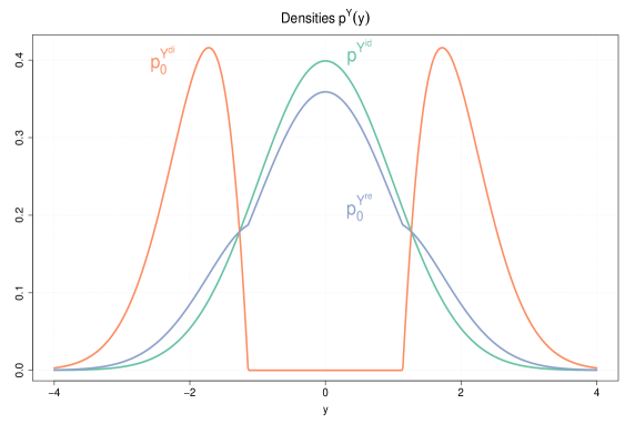
Figure 1: Densities of $P^{Y^{\rm\scriptscriptstyle id}}$, $P_{0}^{Y^{\rm\scriptscriptstyle re}}$, $P_{0}^{Y^{\rm\scriptscriptstyle di}}$ for ${P^{X}}={P^{\varepsilon}}={\cal N}(0,1)$, $r=0.1$; note the “thin” tails.

Remark 3.3.

• Without using this name, SO neighborhoods have already been used by Birmiwal and Shen (1993) and Birmiwal and Papantoni-Kazakos (1994), although only in a one-dim. model.

• Explicit solutions to robust optimization problems in a finite sample setting are rare, which is why one usually appeals to asymptotics instead. Important exceptions are Huber (1968), Huber and Strassen (1973), and even there, in the former case one is limited to a special loss function and to one dimension. Our results however are valid in a finite sample context and in whole generality.

• Although the structure of our model resembles a location model—interpreting $X$ as a random location parameter—our saddle-point differs from the one obtained in Huber (1964). To see this, let us look at the tails of the least favorable $P_{0}^{Y^{\rm\scriptscriptstyle re}}$ assuming a Gaussian model for simplicity: while in Huber’s setting the tails decay as $ce^{-k|x|}$ for some $c,k>0$, in our setting they decay as $c^{\prime}|x|e^{-x^{2}/2}$ so appear even “less harmful” than in the location case.

• Attempts to solve corresponding optimization problems in a (narrow-sense) AO neighborhood are much more difficult and only partial results in this context have been obtained in Donoho (1978), Bickel (1981), and Bickel and Collins (1983); in particular one knows, that in the setup of our example the least favorable $\tilde{P}^{\varepsilon}=P_{0}^{\varepsilon^{\rm\scriptscriptstyle di}}$ must be discrete with only possible accumulation points $\pm\infty$. In addition, existence of a saddle-point follows from abstract compactness and continuity arguments, but in order to obtain specific solutions one has to recur to numeric approximation techniques as e.g. worked out in Ruckdeschel (2001, sec. 8.3); in particular, one obtains redescending optimal filters.

• Redescenders are also used in the ACM filter by Masreliez and Martin (1977) which formally translates the Huber (1964) minimax variance result to this dynamic setting (formally, because of the randomness of the “location parameter” $\Delta X$). It should be noted though that the least-favorable SO-situation for the ACM then is not in the tails but rather where the corresponding $\psi$ function takes its maximum in absolute value. An SO outlier could easily place contaminating mass on this maximum, while this is much harder if not impossible to achieve in a (narrow-sense) AO situation. Hence in simulations where we produce “large” outliers, the ACM filter tends to outperform the rLS filter, as these “large” outliers are least favorable for the rLS but not for the ACM. The “inliers” producing the least favorable situation for the ACM on the other hand will be much harder to detect on naïve data inspection than “large” outliers, in particular in higher dimensions.

3.3 Back in the $\Delta X$ Model for $t>1$

So far, in this section, we have ignored the fact that our $X$ in model (3.9) resp. $\Delta X_{t}$ in the SSM context will stem from a past which has already used our robustified version of the Kalman filter. In particular, the law of $\Delta X_{t}$ (even in the ideal model) is not straightforward and hence (ideal) conditional expectation appearing in the optimal solution $f_{0}$ in Theorem 3.2 in practice are not so easily computable.

3.3.1 Approaches to go back

The issue to assess the law $\Delta X_{t}$ from a non-linear filter past is common to other robustifications, and hence there already exist a couple of approaches to deal with it: Masreliez and Martin (1977) and Martin (1979) assume ${\cal L}(\Delta X_{t})$ normal and propose using robust location estimators (with redescending $\psi$-function) as alternatives to the linear correction step. Contradicting this assumption in the rLS case, we have the following proposition

Proposition 3.4.

Whenever in one correction step in the $\Delta X_{t}$ past one has used the rLS-filter, then $\{\Delta X_{t}\}$ (as a process) cannot be normally distributed; this assertion cannot even hold asymptotically, as long as

$$0<\liminf_{t}b_{t}\leq\limsup_{t}b_{t}<\infty$$ (3.21)

Similar assertions can also be proven for particular $\psi$-functions used in the ACM filter of Masreliez and Martin (1977) and Martin (1979).

Schick (1989) and Schick and Mitter (1994) use Taylor-expansions for non-normal ${\cal L}(\Delta X_{t})$; doing so they end up with stochastic error terms but do not give an indication as to uniform integrability. Hence it is not clear whether the approximation stays valid after integration. More importantly, at time instance $t$, they come up with a bank of (at least $t$) Kalman–filters which is not operational.

Birmiwal and Shen (1993) work with the exact ${\cal L}(\Delta X_{t})$ and hence have to split up the integration according to the the history of outlier occurrences which yields $2^{t}$ different terms—which is not operational either.

Remark 3.5.

One of the features of the ideal Gaussian model is that $\mathop{\rm{{}E{}}}\nolimits_{\rm\scriptscriptstyle id}[\Delta X_{t}|Y_{1:t}]$ is Markovian in the sense that $\mathop{\rm{{}E{}}}\nolimits_{\rm\scriptscriptstyle id}[\Delta X_{t}|Y_{1:t}]=\mathop{\rm{{}E{}}}\nolimits_{\rm\scriptscriptstyle id}[\Delta X_{t}|\Delta Y_{t}]$ hence only depends on the one value of $\Delta Y_{t}$. When using bounded correction steps, however, this property gets lost, hence the restriction to strictly recursive procedures as is the rLS filter is a real restriction.

Theorem 3.2 does not make any normality assumptions, but in assertion (3), we have seen that the rLS would result optimal once we can show that $\mathop{\rm{{}E{}}}\nolimits_{\rm\scriptscriptstyle id}[\Delta X_{t}|\Delta Y_{t}]$ for $\Delta X$ stemming from an rLS past is linear. This leads to the question: When is $\mathop{\rm{{}E{}}}\nolimits_{\rm\scriptscriptstyle id}[\Delta X|\Delta Y]$ linear? Omitting time indices $t$, the answer is

Proposition 3.6.

Assume $\mathop{\rm rk}\nolimits({\mathbb{I}}_{p}-MZ)=p$, $p=q$ and $\mathop{\rm rk}\nolimits Z=p$, and that

$${\cal L}_{\rm\scriptscriptstyle id}(\varepsilon)={\cal N}_{q}(0,V),\qquad\varepsilon\mbox{ independent of }\Delta X$$ (3.22)

Then $\mathop{\rm{{}E{}}}\nolimits_{\rm\scriptscriptstyle id}[\Delta X|\Delta Y]$ is linear

$$\iff \!\!\!{\cal L}_{\rm\scriptscriptstyle id}(\Delta X)\quad\mbox{is normal}$$ (3.23)

$$\iff \!\!\!M_{3}(e):=\mathop{\rm{{}E{}}}\nolimits_{\rm\scriptscriptstyle id}\big{[}\big{(}e^{\tau}(\Delta X-\mathop{\rm{{}E{}}}\nolimits[\Delta X|\Delta Y])\big{)}^{3}\,\big{|}\,\Delta Y\!=\!y\big{]}=0\;\;\;\forall\,e\in\mathbb{R}^{p}$$ (3.24)

Remark 3.7.

• Assumption $\mathop{\rm rk}\nolimits({\mathbb{I}}_{p}-MZ)=p$ is fulfilled in most situations; otherwise there is a one-dimensional projection of the filter error that is $0$ almost sure.

• For $Z$ non-invertible, in particular for $p\not=q$, equivalence (3.23) still holds, if we require

  $${\cal L}_{\rm\scriptscriptstyle id}(\Pi\Delta X)={\cal N}_{p}(0,\Pi\Sigma\Pi),\qquad\Pi\Delta X\mbox{ independent of }\bar{\Pi}\Delta X$$ (3.25)

  where $\Pi$ is the projector onto $\ker Z$ and $\bar{\Pi}={\mathbb{I}}_{p}-\Pi$. In fact we prove Proposition 3.6 in this more general case. Assumption (3.25) is needed, as $\Pi\Delta X$ is invisible for $\Delta Y$.

• Equivalence (3.23) together with Proposition 3.4 shows that, stemming from an rLS-past, rLS can only be SO-optimal in the very first time step.

• Simulations however show that rLS gives very reasonable results. So in fact we could/should be close to an ideal linear conditional expectation. “Closeness” to linearity could be quantified by the second derivative $\partial^{2}/\partial y^{2}\mathop{\rm{{}E{}}}\nolimits_{\rm\scriptscriptstyle id}[\Delta X|\Delta Y=y]$, which in fact leads us to expression (3.24).

• Equivalence (3.24), i.e.; conditional unskewedness of $\Delta X$, is somewhat surprising, as it seems much weaker than normality of the prediction error.

• Condition (3.22) could be relaxed to $\varepsilon~{}\sim P$, $P$ some infinitely divisible distribution, and the normality assumption in (3.25) be dropped. Equivalence (3.23) would then become: For each $M\in\mathbb{R}^{p\times q}$ there can be at most one distribution $Q=Q(M,P)$ on $\mathbb{B}^{p}$, such that $\mathop{\rm{{}E{}}}\nolimits[\Delta X|\Delta Y]=M\Delta Y$ for ${\cal L}(\bar{\Pi}\Delta X)=Q$; for $p=q=1$ and $Z\not=0$, there always is such a $Q$; see Ruckdeschel (2001, Thm. 1.3.1).

3.3.2 A test for linearity

In particle filter context where you simulate many stochastically independent filter realizations in parallel, Proposition 3.6 suggests the following test for linearity/normality:

Proposition 3.8.

Let $\Delta X_{i}^{\natural}$, $i=1,\ldots,n$ be an i.i.d. sample from ${\cal L}(\Delta X_{t})$, the law of the prediction errors of some filter at time $t$; let $\Sigma=\mathop{\rm Cov}\nolimits(\Delta X_{t})$, $\sigma^{2}$ its maximal eigenvalue and $e$ a corresponding eigenvector (of norm $1$); let $\hat{\Sigma}_{n}$, $\hat{\sigma}_{n}^{2}$, and $\hat{e}_{n}$ the corresponding empirical counter parts (all assumed consistent). Define the test statistic $T_{n}=\frac{1}{n}\sum_{i=1}^{n}(\hat{e}_{n}^{\tau}\Delta X_{i}^{\natural})^{3}$. Then under normality of ${\cal L}(\Delta X_{t})$,

$$\sqrt{n}\,T_{n}\mathrel{\mbox{$\longrightarrow$}\hbox to0.0pt{\hss\raisebox{-0.6458pt}{\makebox[7.5pt]{\scriptsize\rm w}}}}{\cal N}(0,15\sigma^{6})$$ (3.26)

and the test

$$\mathop{\bf\rm{{}I{}}}\nolimits(|T_{n}|>\sqrt{15/n}\,\hat{\sigma}_{n}^{3}u_{\alpha/2})$$ (3.27)

for $u_{\alpha}$ the upper $\alpha$-quantile of ${\cal N}(0,1)$ is asymptotically most powerful among all unbiased level-$\alpha$-tests for testing

$$\mbox{$H_{0}$}\colon\quad\sup_{|e|=1}M_{3}(e)=0\qquad\mbox{vs.}\qquad\mbox{$H_{1}$}\colon\quad\sup_{|e|=1}|M_{3}(e)|>0$$ (3.28)

3.4 Way out: eSO-Neighborhoods

One explanation for the good empirical findings for the rLS is given by a further extension of the original SO-neighborhoods—the extended SO or ${\rm eSO}$–model: In this model, we also allow for model deviations in $X$, i.e.; we assume a realistic $(X^{\rm\scriptscriptstyle re},Y^{\rm\scriptscriptstyle re})$ according to

$$(X^{\rm\scriptscriptstyle re},Y^{\rm\scriptscriptstyle re}):=(1-U)(X^{\rm\scriptscriptstyle id},Y^{\rm\scriptscriptstyle id})+U(X^{\rm\scriptscriptstyle di},Y^{\rm\scriptscriptstyle di})$$ (3.29)

for $X^{\rm\scriptscriptstyle id}\sim P^{X^{\rm\scriptscriptstyle id}}$, $Y^{\rm\scriptscriptstyle id}$ according to equation (3.9), $X^{\rm\scriptscriptstyle di}\sim P^{X^{\rm\scriptscriptstyle di}}$, $Y^{\rm\scriptscriptstyle di}\sim P^{Y^{\rm\scriptscriptstyle di}}$, $U\sim{\rm Bin}(1,r_{\rm\scriptscriptstyle eSO})$, where

$$U\mbox{ and }(X^{\rm\scriptscriptstyle id},Y^{\rm\scriptscriptstyle id})\;\mbox{ independent as well as (mutually) }U,X^{\rm\scriptscriptstyle di},Y^{\rm\scriptscriptstyle di}$$ (3.30)

and the joint law $P^{X^{\rm\scriptscriptstyle id},Y^{\rm\scriptscriptstyle id}}$ and the radius $r=r_{\rm\scriptscriptstyle eSO}$ are known, while $P^{X^{\rm\scriptscriptstyle di}},P^{Y^{\rm\scriptscriptstyle di}}$ are arbitrary, unknown and uncontrollable; however, we assume that

$$\mathop{\rm{{}E{}}}\nolimits_{\rm\scriptscriptstyle di}X^{\rm\scriptscriptstyle di}=\mathop{\rm{{}E{}}}\nolimits_{\rm\scriptscriptstyle id}X^{\rm\scriptscriptstyle id},\qquad\mathop{\rm{{}E{}}}\nolimits_{\rm\scriptscriptstyle di}|X^{\rm\scriptscriptstyle di}|^{2}\leq G$$ (3.31)

for some known $0<\mathop{\rm{{}E{}}}\nolimits_{\rm\scriptscriptstyle id}|X^{\rm\scriptscriptstyle id}|^{2}\leq G<\infty$, and accordingly define

$$\!\!\!\!{\cal U}^{{\rm\scriptscriptstyle eSO}}(r):=\!\!\!\!\bigcup_{0\leq s\leq r}\!\!\partial{\cal U}^{\rm\scriptscriptstyle eSO}(s),\quad\partial{\cal U}^{\rm\scriptscriptstyle eSO}(r):=\{\;{\cal L}(X^{\rm\scriptscriptstyle re},Y^{\rm\scriptscriptstyle re})\;\mbox{acc. to \eqref{eso1}--\eqref{esogl}}\;\}$$ (3.32)

Remark 3.9.

At first glance, moment condition (3.31) seems to violate (distributional) robustness; however, this condition has not been introduced to induce a higher degree of robustness, but rather to extend the applicability of Theorem 3.2.

Theorem 3.10 (minimax-eSO).

The pair $(f_{0},P_{0}^{Y^{\rm\scriptscriptstyle di}})$, optimal in the Minimax-SO-problem to radius $r_{\rm\scriptscriptstyle SO}=r$ from Theorem 3.2, extended to $\big{(}f_{0},P_{0}^{Y^{\rm\scriptscriptstyle di}}\otimes P_{0}^{X^{\rm\scriptscriptstyle di}}\big{)}$ for any $P_{0}^{X^{\rm\scriptscriptstyle di}}$ such that $\mathop{\rm{{}E{}}}\nolimits_{\rm\scriptscriptstyle di}|X^{\rm\scriptscriptstyle di}|^{2}=G$, remains a saddle-point in the corresponding Minimax-Problem on the ${\rm eSO}$-neighborhood ${\cal U}^{\rm\scriptscriptstyle eSO}$ to the same radius $r$—no matter what bound $G$ in equation (3.31) holds. The value of the minimax risk is

$$\mathop{\rm{}tr{}}\mathop{\rm Cov}\nolimits_{\rm\scriptscriptstyle id}X^{\rm\scriptscriptstyle id}+r(G-\mathop{\rm{{}E{}}}\nolimits_{\rm\scriptscriptstyle id}|X^{\rm\scriptscriptstyle id}|^{2})-(1-r)\mathop{\rm{{}E{}}}\nolimits_{\rm\scriptscriptstyle id}\big{[}\,|D(Y^{\rm\scriptscriptstyle id})|^{2}w_{r}(Y^{\rm\scriptscriptstyle id})\big{]}$$ (3.33)

As an application of Theorem 3.10, we now invoke a coupling idea: In the Gaussian setup, i.e.; we assume (2.3), we no longer regard the (SO–) saddle-point solution to an ${\cal U}(r)$-neighborhood around ${\cal L}(\Delta X)$ stemming from an rLS-past, but use Theorem 3.10 as follows:

Proposition 3.11.

Assume that for each time $t$ there is a (fictive) random variable $\Delta X^{\cal N}\sim{\cal N}_{p}(0,\Sigma)$ such that $\Delta X_{t}^{\rm\scriptscriptstyle rLS}$ stemming from an rLS-past can be considered an $X^{\rm\scriptscriptstyle di}$ in the corresponding ${\rm eSO}$-neighborhood around $\Delta X^{\cal N}$ with radius $r$. Then, rLS is exactly minimax for each time $t$.

Remark 3.12.

• Existence of $\Delta X^{\cal N}\sim{\cal N}_{p}(0,\Sigma)$ in a general setting is not yet proved. To this end one has to show moment condition (3.31) and that

  $$\sup\nolimits_{\lambda}\big{(}p^{\Delta X_{t}^{\cal N}}\,/\,p^{\Delta X_{t}}\big{)}\geq 1-r$$ (3.34)

  where $p^{\Delta X_{t}^{\cal N}}$, $p^{\Delta X_{t}}$ are the corresponding Lebesgue densities and $\sup\nolimits_{\lambda}$ is the corresponding essential supremum w.r.t. Lebesgue measure in the respective dimension. Clearly condition (3.34) is the difficulty, while condition (3.31) is not hard to fulfill—we only need to check that $\mathop{\rm{{}E{}}}\nolimits_{\rm\scriptscriptstyle id}\Delta X_{t}=0$, which for the rLS follows from symmetry of the distributions in the ideal model, and that the second moment is bounded—which also clearly holds.

• As to the choice of covariance $\Sigma$ for $\Delta X_{t}^{\cal N}$, we have two candidates: $\Sigma=\mathop{\rm Cov}\nolimits\Delta X_{t}^{\rm\scriptscriptstyle rLS}$ and $\Sigma=\Sigma_{t|t-1}$ from the classical Kalman filter. While the former takes up the actual error covariances, the latter is much easier to compute. In our numerical examples in Ruckdeschel (2001), we could not find any significant advantages for the former in terms of precision and hence propose the latter for computational reasons.

• For $p=1$, (3.34) could be checked numerically in a number of models, cf.  Ruckdeschel (2001, Table 8.1). For $p>1$, particle filter techniques should be helpful.

4 IO-optimality

In this section, we translate the preceding optimality results to the IO situation. We have already noted that in this case, instead of attenuating (the influence of) a dubious observation we would rather want to follow an IO outlier as fast as possible. It is well-known that the Kalman filter tends to be too inert for this task and faster tracking filters are needed. To do so, let us go back to our “Bayesian” model (3.9) but now we specify the transition densities $\pi(y,x)$ to come from an observation $Y$ which is built up additively as

$$Y=X+\varepsilon$$ (4.1)

Equation (4.1) reveals a remarkable symmetry of $X$ and $\varepsilon$ which we are going to exploit now: Apparently

$$\mathop{\rm{{}E{}}}\nolimits[X|Y]=Y-\mathop{\rm{{}E{}}}\nolimits[\varepsilon|Y]$$ (4.2)

This is helpful if we are now assuming that $\varepsilon$ will be ideally distributed, and instead the states $X$ get corrupted. To this end, we retain the SO-model from the preceding sections, i.e., $Y^{\rm\scriptscriptstyle id}$ will be replaced from time to time by $Y^{\rm\scriptscriptstyle di}$. Contrary to the AO formulation however, we now assume that this replacement by $Y^{\rm\scriptscriptstyle di}$ reflects a corresponding change in $X$, as we now want to track the distorted signal. As a consequence this gives the following IO-version of the minimax problem (where the only visible difference is the superscript “${\rm\textstyle re}$” for $X$).

$$\max\nolimits_{{\cal U}}\,\mathop{\rm{{}E{}}}\nolimits_{\scriptscriptstyle\rm re}|X^{\rm\scriptscriptstyle re}-f(Y^{\rm\scriptscriptstyle re})|^{2}=\min\nolimits_{f}{}!$$ (4.3)

But, using $X^{\rm\scriptscriptstyle re}=Y^{\rm\scriptscriptstyle re}-\varepsilon$, and setting $\tilde{f}(y)=y-f(y)$ we obtain the equivalent formulation

$$\max\nolimits_{{\cal U}}\,\mathop{\rm{{}E{}}}\nolimits_{\scriptscriptstyle\rm re}|\varepsilon-\tilde{f}(Y^{\rm\scriptscriptstyle re})|^{2}=\min\nolimits_{\tilde{f}}{}!$$ (4.4)

and we are back in the situation of subsection (3.2) with the respective rôles of $X$ and $\varepsilon$ interchanged. That is; the corresponding theorems translate word by word. Skipping the Lemma 5 solution we obtain

Theorem 4.1 (Minimax-IO).

1. In this situation, there is a saddle-point $(f_{1},P_{1}^{Y^{\rm\scriptscriptstyle di}})$ for Problem (4.3)

   $$f_{1}(y) := y-\tilde{D}(y)\min\{1,\tilde{\rho}/\big{|}\tilde{D}(y)\big{|}\}$$ (4.5)

   $$P_{1}^{Y^{\rm\scriptscriptstyle di}}(dy) := \textstyle\frac{1-r}{r}(\big{|}\tilde{D}(y)\big{|}\,\big{/}\tilde{\rho}\,-1)_{\scriptscriptstyle+}\,\,P^{Y^{\rm\scriptscriptstyle id}}(dy)$$ (4.6)

   where $\tilde{\rho}>0$ ensures that $\int\,P_{1}^{Y^{\rm\scriptscriptstyle di}}(dy)=1$ and

   $$\tilde{D}(y)=y-\mathop{\rm{{}E{}}}\nolimits_{\scriptscriptstyle\rm id}[X|Y=y]$$ (4.7)

2. If $\mathop{\rm{{}E{}}}\nolimits_{\scriptscriptstyle\rm id}[X|Y]$ is linear in $Y$, i.e.; $\mathop{\rm{{}E{}}}\nolimits_{\scriptscriptstyle\rm id}[X|Y]=MY$ for some matrix $M$, then necessarily

   $$M=M^{0}=\mathop{\rm Cov}\nolimits(X,Y)\mathop{\rm Var}\nolimits Y^{-}$$ (4.8)

   —or in the SSM formulation: $M^{0}$ is just the classical Kalman gain and $f_{1}$ the (one-step) rLS.IO defined below.

Note that contrary to Theorem 3.2 where $\mathop{\rm{{}E{}}}\nolimits X$ need not be $0$, here $\mathop{\rm{{}E{}}}\nolimits\varepsilon=0$, which simplifies the definition of $\tilde{D}$ in (4.7). Details on how to use this for a corresponding IO-robust variant of rLS are given in Ruckdeschel (2010).

5 Conclusion and Outlook

In the extremely flexible class of dynamic models consisting in SSMs we were able to obtain optimality results for filtering. In this generality this is a novelty. We stress the fact that our filters are non-iterative, recursive, hence fast, and valid for higher dimensions.

So far, we have not said much about the implementation of these filters. rLS.AO was originally implemented to XploRe, compare Ruckdeschel (2000). In an ongoing project with Bernhard Spangl, BOKU, Vienna, and Irina Ursachi (ITWM), we are about to implement the rLS filter to R, (R Development Core Team (2010)), more specifically to an R-package robKalman, the development of which is done under r-forge project https://r-forge.r-project.org/projects/robkalman/, (R-Forge Administration and Development Team (2008)). Under this address you will also find a preliminary version available for download.

In an extra paper, which for the moment is available as technical report, Ruckdeschel (2010), we also check the properties of our filters at simulations and discuss the extension of these optimally-robust filters to a filter that combines the two types (for system-endogenous and -exogenous outlier situation). This hybrid filter is capable to treat (wide-sense) IO’s and AO’s simultaneously—albeit with minor delay.

6 Proofs

Proof to Lemma 3.1

We use the fact that for $0\leq a,b,c,d$, $(a+b)/(c+d)\leq\max(a/c,b/d)$. Hence

$$\rho_{0}(s)\leq\max\{A_{s}/A_{r_{l}},B_{s}/B_{r_{u}}\}$$ (6.1)

Equation (3.3) shows that $b(r)$ is (strictly) decreasing in $r$ (for $r>0$) from $\infty$ to $0$. Hence $A_{r}$ is increasing in $r$, and $B_{r}$ decreasing, $B_{r}$ from $\infty$ to $0$. By dominated convergence $b(r)$, and hence $A_{r}$ and $B_{r}$ are continuous in $r$. Thus existence of $\bar{r}_{0}$ follows. For $r_{u}=1$, one argues letting $r_{n}\in[0,1)$ tend to $1$. To show equality in (6.1), we parallel Kohl (2005, Lemma 2.2.3), and first show that for $r\geq s$, $s$ fixed, $\rho(r,s)$ is increasing and correspondingly, for $r\leq s$, $s$ fixed, decreasing, which entails (3.8): Let $0\leq s<r_{1}<r_{2}\leq 1$. Then by monotony of $A_{r}$, $B_{r}$, $(A_{s}B_{s}^{-1}+r_{1})^{-1}\geq(A_{r_{1}}B_{r_{1}}^{-1}+r_{1})^{-1}$; multiplying this inequality with $(r_{2}-r_{1})$, we get $(r_{2}-r_{1})B_{s}(A_{s}+r_{1}B_{s})^{-1}\geq(r_{2}-r_{1})B_{r_{1}}(A_{r_{1}}+r_{1}B_{r_{1}})^{-1}$. Now, due to optimality of $A_{r}+rB_{r}$ for radius $r$,

$$0 \leq \frac{(r_{2}-r_{1})B_{s}}{A_{s}+r_{1}B_{s}}-\frac{(r_{2}-r_{1})B_{r_{1}}+A_{r_{2}}+r_{2}B_{r_{2}}-A_{r_{1}}-r_{2}B_{r_{1}}}{A_{r_{1}}+r_{1}B_{r_{1}}}=$$

$$= (r_{2}-r_{1})B_{s}(A_{s}+r_{1}B_{s})^{-1}-\big{(}A_{r_{2}}+r_{2}B_{r_{2}}\big{)}(A_{r_{1}}+r_{1}B_{r_{1}})^{-1}+1$$

Multiplying with $(A_{s}+r_{1}B_{s})/(A_{r_{2}}+r_{2}B_{r_{2}})$, we obtain indeed $\rho(r_{2},s)\geq\rho(r_{1},s)$, and similarly for $0\geq s>r_{1}>r_{2}\geq 1$. Next, for $\tilde{r}_{0}$ least favorable, we show that for $r$ fixed, and $s\geq r$, $\rho(r,s)$ is increasing and correspondingly, for $s\leq r$, decreasing: Let $0\leq r<r_{1}<r_{2}\leq 1$. Then, due to optimality of $A_{r_{1}}-r_{1}B_{r_{1}}$,

$$A_{r_{2}}+rB_{r_{2}}-A_{r_{1}}+rB_{r_{1}}=$$

$$\quad=(r_{1}-r)(B_{r_{1}}-B_{r_{2}})+A_{r_{2}}+r_{1}B_{r_{2}}-A_{r_{1}}-r_{1}B_{r_{1}}\geq 0$$

and similarly for $0\geq r>r_{1}>r_{2}\geq 1$. For the last assertion, note that by (3.3), $b(1)=0$, hence $B_{1}=0$. Hence $\max\big{\{}A_{s}/A_{r_{l}},B_{s}/B_{1}\big{\}}=\infty$ for $s<1$, while for $s=1$, we get $\rho_{0}(1)=\max\{A_{1}/A_{r_{l}},1\}=1$. ∎

Proof to Theorem 3.2

(1) Let us solve $\max_{\partial{\cal U}}\min_{f}{}[\ldots]$ first, which amounts to $\min_{\partial{\cal U}}\mathop{\rm{{}E{}}}\nolimits_{\scriptscriptstyle\rm re}[\big{|}\mathop{\rm{{}E{}}}\nolimits_{\scriptscriptstyle\rm re}[X|Y^{\rm\scriptscriptstyle re}]\big{|}^{2}]$. For fixed element $P^{Y^{\rm\scriptscriptstyle di}}$ assume w.l.o.g. that $\mu\gg P^{Y^{\rm\scriptscriptstyle di}}$ for $\mu$ from (3.9)—otherwise we replace $\mu$ by $\mu+P^{Y^{\rm\scriptscriptstyle di}}$; this gives us a $\mu$-density $q(y)$ of $P^{Y^{\rm\scriptscriptstyle di}}$. Determining the joint (real) law $P^{X,Y^{\rm\scriptscriptstyle re}}(dx,dy)$ as

$$P(X\!\in\!A,Y^{\rm\scriptscriptstyle re}\!\in\!B)=\!\!\int\!\!\mathop{\bf\rm{{}I{}}}\nolimits_{A}(x)\mathop{\bf\rm{{}I{}}}\nolimits_{B}(y)[(1\!-\!r)\pi(y,x)+rq(y)]\,P^{X}(dx)\,\mu(dy)$$ (6.2)

we deduce that $\mu(dy)$-a.e.

$$\mathop{\rm{{}E{}}}\nolimits_{\rm\scriptscriptstyle re}[X|Y^{\rm\scriptscriptstyle re}\!\!=\!y]=\frac{rq(y)\!\mathop{\rm{{}E{}}}\nolimits X\!+\!(1\!-\!r)p^{Y^{\rm\scriptscriptstyle id}}(y)\mathop{\rm{{}E{}}}\nolimits_{\scriptscriptstyle\rm id}[X|Y]}{rq(y)+(1-r)p^{Y^{\rm\scriptscriptstyle id}}(y)}\!=:\!\frac{a_{1}q(y)\!+\!a_{2}(y)}{a_{3}q(y)\!+\!a_{4}(y)}$$ (6.3)

Hence we have to minimize

$$F(q):=\int\frac{|a_{1}q(y)+a_{2}(y)|^{2}}{a_{3}q(y)+a_{4}(y)}\,\,\mu(dy)$$

in $M_{0}=\{q\in L_{1}(\mu)\,|\;q\geq 0,\;\int q\,d\mu=1\}$. To this end, we note that $F$ is convex on the non-void, convex cone $M=\{q\in L_{1}(\mu)\,|\;q\geq 0\}$ so, for some $\tilde{\rho}\geq 0$, we may consider the Lagrangian

$$L_{\tilde{\rho}}(q):=F(q)+\tilde{\rho}\int q\,d\mu$$ (6.4)

for some positive Lagrange multiplier $\tilde{\rho}$. Pointwise minimization in $y$ of $L_{\tilde{\rho}}(q)$ gives

$$q_{s}(y)=\textstyle\frac{1-r}{r}(\big{|}D(y)\big{|}\big{/}s\,-1)_{\scriptscriptstyle+}\,\,p^{Y}(y)$$

for some constant $s=s(\tilde{\rho})=(\,|\mathop{\rm{{}E{}}}\nolimits X|^{2}+\tilde{\rho}/r)^{1/2}$, Pointwise in $y$, $\hat{q}_{s}$ is antitone and continuous in $s\geq 0$ and $\lim_{s\to 0[\infty]}q_{s}(y)=\infty[0]$, hence by monotone convergence,

$$H(s)=\int\hat{q}_{s}(y)\,\mu(dy)$$

too, is antitone and continuous and $\lim_{s\to 0[\infty]}H(s)=\infty[0]$. So by continuity, there is some $\rho\in(0,\infty)$ with $H(\rho)=1$. On $M_{0}$, $\int q\,d\mu=1$, but $\hat{q}_{\rho}=q_{s=\rho}\in M_{0}$ and is optimal on $M\supset M_{0}$ hence it also minimizes $F$ on $M_{0}$. In particular, we get representation (3.17) and note that, independently from the choice of $\mu$, the least favorable $P_{0}^{Y^{\rm\scriptscriptstyle di}}$ is dominated according to $P_{0}^{Y^{\rm\scriptscriptstyle di}}\ll P^{Y^{\rm\scriptscriptstyle id}}$, i.e.; non-dominated $P^{Y^{\rm\scriptscriptstyle di}}$ are even easier to deal with.

As next step we show that

$$\max\nolimits_{\partial{\cal U}}\min\nolimits_{f}{}[\ldots]=\min\nolimits_{f}{}\max\nolimits_{\partial{\cal U}}[\ldots]$$ (6.5)

To this end we first verify (3.16) determining $f_{0}(y)$ as $f_{0}(y)=\mathop{\rm{{}E{}}}\nolimits_{\scriptscriptstyle{\rm re};\hat{P}}[X|Y^{\rm\scriptscriptstyle re}=y]$. Writing a sub/superscript “${{\rm re;}\,P}$” for evaluation under the situation generated by $P=P^{Y^{\rm\scriptscriptstyle di}}$ and $\hat{P}$ for $P_{0}^{Y^{\rm\scriptscriptstyle di}}$, we obtain the the risk for general $P$ as

$${\rm MSE}_{\scriptscriptstyle{{\rm re;}\,P}}[f_{0}(Y^{\scriptscriptstyle{\rm re},\,P})] = (1-r)\mathop{\rm{{}E{}}}\nolimits_{\rm\scriptscriptstyle id}\big{|}X-f_{0}(Y^{\rm\scriptscriptstyle id})\big{|}^{2}+r\mathop{\rm{}tr{}}\mathop{\rm Cov}\nolimits X+$$ (6.6)

$$\quad+r\,\mathop{\rm{{}E{}}}\nolimits_{P}\min(|D(Y^{\scriptscriptstyle{\rm di;},q})|^{2},\rho^{2})$$

This is maximal for any $P$ that is concentrated on the set $\big{\{}\,|D(Y^{\scriptscriptstyle{\rm di;},q})|>\rho\,\big{\}}$, which is true for $\hat{P}$. Hence (6.5) follows, as for any contaminating $P$

$${\rm MSE}_{\scriptscriptstyle{{\rm re;}\,P}}[f_{0}(Y^{\scriptscriptstyle{{\rm re;}\,P}}]\leq{\rm MSE}_{\scriptscriptstyle{{\rm re;}\,\hat{P}}}[f_{0}(Y^{\scriptscriptstyle{{\rm re;}\,\hat{P}}})]$$

Finally, we pass over from $\partial{\cal U}$ to ${\cal U}$: Let $f_{r}$, $\hat{P}_{r}$ denote the components of the saddle-point for $\partial{\cal U}(r)$, as well as $\rho(r)$ the corresponding Lagrange multiplier and $w_{r}$ the corresponding weight, i.e., $w_{r}=w_{r}(y)=\min(1,{\rho(r)}\,/\,{|D(y)|})$. Let $R(f,P,r)$ be the MSE of procedure $f$ at the SO model $\partial{\cal U}(r)$ with contaminating $P^{Y^{\rm\scriptscriptstyle di}}=P$. As can be seen from (3.17), $\rho(r)$ is antitone in $r$; in particular, as $\hat{P}_{r}$ is concentrated on $\{|D(Y)|\geq\rho(r)\}$ which for $r\leq s$ is a subset of $\{|D(Y)|\geq\rho(s)\}$, we obtain

$$R(f_{s},\hat{P}_{s},s)=R(f_{s},\hat{P}_{r},s)\qquad\mbox{for}\;r\leq s$$

Note that $R(f_{s},P,0)=R(f_{s},Q,0)$ for all $P,Q$—hence passage to $\tilde{R}(f_{s},P,r)=R(f_{s},P,r)-R(f_{s},P,0)$ is helpful—and that

$$\mathop{\rm{}tr{}}\mathop{\rm Cov}\nolimits X=\mathop{\rm{{}E{}}}\nolimits_{\rm\scriptscriptstyle id}\Big{[}\mathop{\rm{}tr{}}\mathop{\rm Cov}\nolimits_{\rm\scriptscriptstyle id}[X|Y^{\rm\scriptscriptstyle id}]+|D(Y^{\rm\scriptscriptstyle id})|^{2}\Big{]}$$ (6.7)

Abbreviate $\bar{w}_{s}(Y^{\rm\scriptscriptstyle id})=1-\big{(}1-w_{s}(Y^{\rm\scriptscriptstyle id})\big{)}^{2}\geq 0$ to see that

$$\tilde{R}(f_{s},P,r)=r\Big{\{}\mathop{\rm{{}E{}}}\nolimits_{\rm\scriptscriptstyle id}\Big{[}|D(Y^{\rm\scriptscriptstyle id})|^{2}\bar{w}_{s}(Y^{\rm\scriptscriptstyle id})\Big{]}+\mathop{\rm{{}E{}}}\nolimits_{P}\min(|D(Y^{\rm\scriptscriptstyle id})|,\rho(s))^{2}\,\Big{\}}\leq$$

$$\leq r\Big{\{}\mathop{\rm{{}E{}}}\nolimits_{\rm\scriptscriptstyle id}\Big{[}|D(Y^{\rm\scriptscriptstyle id})|^{2}\bar{w}_{s}(Y^{\rm\scriptscriptstyle id})\Big{]}+\rho(s)^{2}\,\Big{\}}=\tilde{R}(f_{s},\hat{P}_{r},r)<\tilde{R}(f_{s},\hat{P}_{s},s)$$

Hence the saddle-point extends to ${\cal U}(r)$; in particular the maximal risk is never attained in the interior ${\cal U}(r)\setminus\partial{\cal U}(r)$. (3.19) follows by plugging in the results.

(2) Let $\tilde{f}(Y)=f(Y)-\mathop{\rm{{}E{}}}\nolimits X$, and $X^{0}=X-\mathop{\rm{{}E{}}}\nolimits X$; then (3.15) becomes

$$\mathop{\rm{{}E{}}}\nolimits_{\scriptscriptstyle\rm id}|X^{0}-\tilde{f}(Y)|^{2}=\min\nolimits_{\tilde{f}}{}!\quad\mbox{s.t.}\;\sup\nolimits_{\cal U}\big{|}\mathop{\rm{{}E{}}}\nolimits_{\scriptscriptstyle\rm re}\tilde{f}(Y^{\rm\scriptscriptstyle re})\big{|}\leq b$$ (6.8)

The assertion follows upon noting that $\sup_{\cal U}|\mathop{\rm{{}E{}}}\nolimits_{\rm\scriptscriptstyle re}\tilde{f}|=\sup|\tilde{f}|$ (to be shown just as in Rieder (1994, chap. 5)) and writing

$$\mathop{\rm{{}E{}}}\nolimits_{\scriptscriptstyle\rm id}|X^{0}-\tilde{f}(Y)|^{2}=\mathop{\rm{{}E{}}}\nolimits_{\scriptscriptstyle\rm id}\Big{[}\mathop{\rm{{}E{}}}\nolimits[|X^{0}-\tilde{f}(Y)|^{2}\,\Big{|}\,Y]\Big{]}$$

—minimize the inner expectation subject to $\big{|}\tilde{f}(Y^{\rm\scriptscriptstyle re})\big{|}\leq b$ pointwise in $Y$.

(3) If $\mathop{\rm{{}E{}}}\nolimits_{\scriptscriptstyle\rm id}[X|Y]$ is linear in $Y$, the corresponding optimal matrix $M^{0}$ is just the respective Fourier coefficient, i.e.; $\mathop{\rm Cov}\nolimits(X,Y)\mathop{\rm Var}\nolimits Y^{-}$. We have already recalled that the classical Kalman filter is optimal among all linear filters; hence the corresponding Kalman gain $M^{0}$ is then the optimal linear transformation in the SSM context. ∎

Remark 6.1.

• Birmiwal and Shen (1993) proceed similarly for their result. However, they invoke a minimax result by Ferguson (1967) which in our infinite dimensional setting is not applicable. Also their setting is restricted to one dimension, and they assume Lebesgue densities right away—also in the contaminated situation. In particular, they do not realize the connection to the exact conditional mean present in equation (3.18).

• For an alternative proof, see Ruckdeschel (2001, pp.156–163): It uses Rieder (1994, App. B), showing existence of Lagrange multipliers in (1) by abstract compactness and continuity arguments.

• The fact that the solutions to Problems (3.14) and (3.15) coincide parallels the situation in the estimation problem for a one-dimensional location parameter.

Proof to Proposition 3.4

Recall that by the Cramér-Lévy Theorem (cf.  Feller (1971, Thm. 1, p. 525)) the sum of two independent random variables has Gaussian distribution iff each summand is Gaussian. This can easily be translated into a corresponding asymptotic statement, cf.  Ruckdeschel (2001, Prop. A.2.4), i.e.; the sum of two independent random variables converges weakly to a Gaussian distribution iff each summand converges weakly to a Gaussian distribution. We first consider (for fixed $t$, omitted from notation where clear) the filter error,

$$\widetilde{\Delta X}:=X_{t}-X_{t|t}=\Delta X-H_{b}(M^{0}\Delta Y)$$

where we assume $\Delta X$, $\varepsilon$, and $v$ normal. Then for the conditional law of $\widetilde{\Delta X}$ given $\Delta Y$ is ${\cal N}_{p}(g,({\mathbb{I}}_{p}-M^{0}Z)\Sigma)$ for $\Sigma=\mathop{\rm Cov}\nolimits\Delta X$ and $g:=M^{0}\Delta Y-H_{b}(M^{0}\Delta Y)=\big{(}\big{|}M^{0}\Delta Y\big{|}-b\big{)}_{\scriptscriptstyle+}$. Hence

$${\cal L}(\widetilde{\Delta X})={\cal L}(g)\ast{\cal N}_{p}(0,({\mathbb{I}}_{p}-M^{0}Z)\Sigma)$$

which by Cramér-Lévy cannot be normal, as $g$ is obviously not normal. Consequently $\Delta X_{t+1}=F_{t+1}\widetilde{\Delta X_{t}}+v_{t+1}$ cannot be normal either. Hence starting with normal $\Delta X_{t}$ and $\varepsilon_{t}$, $\Delta X_{t+1}$ cannot be normal. The same assertion clearly holds if $v_{t}$ is not normal. As by (3.21), $g_{t}$ does neither converge to $0$ nor to $M^{0}\Delta Y$, the asymptotic version of Cramér-Lévy also excludes asymptotic normality. ∎

Remark 6.2.

A similar assertion for the case that $v_{t}$ is normal but not both $\Delta X_{t}$ and $\varepsilon_{t}$ are, seems plausible and we conjecture that this is true; it may also be proven in particular cases, but in general, it is hard to obtain due to the lack of independence of $\Delta X-g$ and $\Delta Y$.

Proof to Proposition 3.6

For the second equivalence in Proposition 3.6 we use the following lemma and a corollary of it:

Lemma 6.3.

Let $\varepsilon\sim{\cal N}_{q}(0,V)$, $X\sim P^{X}$ and for some measurable function $h\colon\mathop{\rm range}(X)\to\mathbb{R}^{q}$ let $Y=h(x)+\varepsilon$. Let $g\in L^{l}_{1}(P^{X})$, i.e., $g\colon\mathop{\rm range}(X)\to\mathbb{R}^{l}$ measurable and $\mathop{\rm{{}E{}}}\nolimits_{P^{X}}|g(X)|<\infty$. Then

$$\frac{\partial}{\partial y}\mathop{\rm{{}E{}}}\nolimits[g(X)|Y=y]=\mathop{\rm Cov}\nolimits[g(x),h(x)|Y=y]V^{-1}$$ (6.9)

Proof.

For simplicity, we only consider $\mathop{\rm rk}\nolimits V=q$; otherwise we may pass to $\varepsilon=A\tilde{\varepsilon}$ for some $\tilde{\varepsilon}\sim{\cal N}_{\tilde{q}}(0,\tilde{V})$ with $\mathop{\rm rk}\nolimits\tilde{V}=\tilde{q}$ and use the generalized inverse $V^{-}$ instead of $V^{-1}$ everywhere in the proof.

Let $p^{\varepsilon}$ be the Lebesgue density of $\varepsilon$ and denote $\Lambda^{\varepsilon}(\varepsilon):=\frac{\partial}{\partial\varepsilon}\log p^{\varepsilon}(\varepsilon)$. Then, no matter whether $\varepsilon$ is Gaussian, it holds that

$$\mathop{\rm{{}E{}}}\nolimits[g(X)|Y=y]=\frac{\int g(x)p^{\varepsilon}(y-h(x))\,P^{X}(dx)}{\int p^{\varepsilon}(y-h(x))\,P^{X}(dx)}$$

As $\varepsilon$ is normal, we may interchange differentiation and integration and obtain that

$$\frac{\partial}{\partial y}\mathop{\rm{{}E{}}}\nolimits[g(X)|Y=y]=\mathop{\rm Cov}\nolimits[g(X),\Lambda^{\varepsilon}(Y-h(X))\,|Y=y]$$

But as $\varepsilon\sim{\cal N}_{q}(0,V)$, it holds that $\Lambda^{\varepsilon}(\varepsilon)=-V^{-1}\varepsilon$, which entails (6.9) as

$$\Lambda^{\varepsilon}(y-h(X))-\mathop{\rm{{}E{}}}\nolimits[\Lambda^{\varepsilon}(Y-h(X))|Y=y]=V^{-1}(h(X)-\mathop{\rm{{}E{}}}\nolimits[h(X)|Y=y])$$

∎

Corollary 6.4.

In our linear time discrete, Euclidean SSM, ommiting indices $t$, assume that $\mathop{\rm rk}\nolimits V=q$ and let

$$U:=V^{-1}Z\Delta X,\quad U^{0}:=U-\mathop{\rm{{}E{}}}\nolimits[U|\Delta Y],\quad\Delta X^{0}:=\Delta X-\mathop{\rm{{}E{}}}\nolimits[\Delta X|\Delta Y]$$ (6.10)

Then

$$\frac{\partial}{\partial y}\mathop{\rm{{}E{}}}\nolimits[\Delta X|\Delta Y=y] = \mathop{\rm Cov}\nolimits(\Delta X,U|\Delta Y=y)$$ (6.11)

$$\frac{\partial^{2}}{\partial y_{j}\partial y_{k}}\mathop{\rm{{}E{}}}\nolimits[\Delta X_{i}|\Delta Y=y] = \mathop{\rm{{}E{}}}\nolimits(\Delta X_{i}^{0}U_{j}^{0}U_{k}^{0}|\Delta Y=y)$$ (6.12)

Proof.

During the proof we will omit $\Delta$ in notation. Equation (6.11) is just plugging in Lemma 6.3. We note that equivalently to (6.9) we could have written

$$\frac{\partial}{\partial y}\mathop{\rm{{}E{}}}\nolimits[X|Y=y]=\mathop{\rm{{}E{}}}\nolimits[X(U^{0})^{\tau}|Y=y]=\mathop{\rm{{}E{}}}\nolimits[XU^{\tau}|Y=y]-\mathop{\rm{{}E{}}}\nolimits[X|Y=y]\mathop{\rm{{}E{}}}\nolimits[U|Y=y]^{\tau}$$

Hence applying Lemma 6.3 for $g(X)=X_{i}U_{j}$ and $g(X)=U_{j}$ to the last two terms we obtain

$$\frac{\partial^{2}}{\partial y_{j}\partial y_{k}}\mathop{\rm{{}E{}}}\nolimits[X_{i}|Y=y] = \mathop{\rm{{}E{}}}\nolimits[X_{i}U_{j}U_{k}^{0}|Y=y]-\mathop{\rm{{}E{}}}\nolimits[X_{i}|Y=y]\mathop{\rm{{}E{}}}\nolimits[U_{j}U_{k}^{0}|Y=y]=$$

$$= \mathop{\rm{{}E{}}}\nolimits[X_{i}^{0}U_{j}U_{k}^{0}|Y=y]=\mathop{\rm{{}E{}}}\nolimits[X_{i}^{0}U_{j}^{0}U_{k}^{0}|Y=y]$$

∎

Proof to Proposition 3.6 Equivalence (3.23):
If ${\cal L}(\Delta X)$ is normal, the uncorrelated random variables $\Pi\Delta X$ and $\bar{\Pi}\Delta X$ are independent and again normal, while the random variables $\Delta X,\Delta Y$ are jointly normal, hence linearity of conditional expectation is a well-known fact.

If $\mathop{\rm{{}E{}}}\nolimits_{\rm\scriptscriptstyle id}[\Delta X|\Delta Y]$ is linear, after subtracting $\mathop{\rm{{}E{}}}\nolimits MZ\Delta X$ from both sides, the defining equation for the conditional expectation $P^{Y}(dy)$-a.e. reads

$$M\int(y-Zx)p^{\varepsilon}(y-Zx)\,P^{X}(dx)=({\mathbb{I}}_{p}-MZ)\int xp^{\varepsilon}(y-Zx)\,P^{X}(dx)$$ (6.13)

Let us introduce $q^{\varepsilon}(y)=yp^{\varepsilon}(y)$ and the signed measure $Q^{X}(dx)=x\,P(dx)$; if we denote the mapping $h\colon\mathbb{R}^{q}\to\mathbb{R},y\mapsto h(y)=\int f(y-Zx)\,G(dx)$ by $f\mathop{\ast_{\scriptscriptstyle Z}}G$, (6.13) becomes

$$Mq^{\varepsilon}\mathop{\ast_{\scriptscriptstyle Z}}P^{X}=({\mathbb{I}}_{p}-MZ)p^{\varepsilon}\mathop{\ast_{\scriptscriptstyle Z}}Q^{X}$$ (6.14)

We pass over to the Fourier transforms (denoted with $\,\hat{\cdot}\,$) for $s\in\mathbb{R}^{p}$, $t\in\mathbb{R}^{q}$

$$\begin{array}[]{ll}\hat{q}^{X}(s)=\int e^{is^{\tau}x}\,Q^{X}(dx),&\quad\hat{p}^{X}(s)=\int e^{is^{\tau}x}\,P^{X}(dx),\\ \hat{q}^{\varepsilon}(t)=\int e^{it^{\tau}x}q^{\varepsilon}(y)\,dy,&\quad\hat{p}^{\varepsilon}(t)=\int e^{it^{\tau}x}p^{\varepsilon}(y)\,dy,\end{array}$$

As usual, convolution translates into products in Fourier space, in our case

$$\widehat{f\mathop{\ast_{\scriptscriptstyle Z}}G}(t)=\hat{f}(t)\hat{G}(Z^{\tau}t),\qquad t\in\mathbb{R}^{q}$$

and hence (6.14) in Fourier space is $M\hat{q}^{\varepsilon}\hat{p}^{X}(Z^{\tau}\,\cdot\,)=({\mathbb{I}}_{p}-MZ)\hat{p}^{\varepsilon}\hat{q}^{X}(Z^{\tau}\,\cdot\,)$. For the derivatives $(\hat{p}^{X})^{\prime}(s)$, $(\hat{p}^{\varepsilon})^{\prime}(t)$ for $s\in\mathbb{R}^{p}$ and $t\in\mathbb{R}^{q}$, we obtain

$$(\hat{p}^{X})^{\prime}(s)=i\,\hat{q}^{X}(s),\qquad(\hat{p}^{\varepsilon})^{\prime}(t)=i\,\hat{q}^{\varepsilon}(t)$$ (6.15)

By assumption, ${\mathbb{I}}_{p}-MZ$ is invertible and $\varepsilon\sim{\cal N}_{q}(0,V)$, hence $\hat{p}^{\varepsilon}(t)=\exp(-t^{\tau}Vt/2)>0$ and together with (6.15), this gives the linear differential equation

$$(\hat{p}^{X})^{\prime}(Z^{\tau}t)=-({\mathbb{I}}_{p}-MZ)^{-1}MVt\hat{p}^{X}(Z^{\tau}t)$$ (6.16)

Fixing any direction $t_{0}$ such that $Z^{\tau}t_{0}\not=0$, this becomes an ODE

$$g^{\prime}(s)=-t_{0}^{\tau}Z({\mathbb{I}}_{p}-MZ)^{-1}MVt_{0}sg(s),\qquad g(0)=1$$

which has a unique solution given by

$$g(s)=\exp(-t_{0}^{\tau}Z({\mathbb{I}}_{p}-MZ)^{-1}MVt_{0}s^{2}/2)$$

This is the characteristic function of a normal distribution, so $Z\Delta X$, hence also $\bar{\Pi}\Delta X$ are normal, and together with (3.25) the assertion follows. On the other hand, $\mathop{\rm Cov}\nolimits Z\Delta X=Z\Sigma Z^{\tau}$, so we have also shown that $Z({\mathbb{I}}_{p}-MZ)^{-1}MV=Z\Sigma Z^{\tau}$, which otherwise is tricky unless assuming $\Sigma$ and $\Delta$ invertible.
Equivalence (3.24):
If $\mathop{\rm{{}E{}}}\nolimits_{\rm\scriptscriptstyle id}[\Delta X|\Delta Y]$ is linear, by equivalence (3.23) $\Delta X$ and $\Delta Y$ are jointly normal with expectation $0$, so the conditional law of $\Delta X$ given $\Delta Y$ is again normal with expectation 0, hence in particular symmetric so the assertion follows.
Now assume

$$\mathop{\rm{{}E{}}}\nolimits\Big{[}\Big{(}e^{\tau}(\Delta X-\mathop{\rm{{}E{}}}\nolimits[\Delta X|\Delta Y])\Big{)}^{3}\,\Big{|}\,\Delta Y\Big{]}=0\qquad\forall\,e\in\mathbb{R}^{p}$$ (6.17)

Apparently, $\mathop{\rm{{}E{}}}\nolimits_{\rm\scriptscriptstyle id}[\Delta X|\Delta Y]$ is linear iff $\partial^{2}/\partial y\partial y^{\tau}\mathop{\rm{{}E{}}}\nolimits_{\rm\scriptscriptstyle id}[\Delta X|\Delta Y]=0.$ But Corollary 6.4 gives (in the notation of (6.10))

$$\frac{\partial^{2}}{\partial y_{j}\partial y_{k}}\mathop{\rm{{}E{}}}\nolimits[\Delta X_{i}|\Delta Y=y]=\mathop{\rm{{}E{}}}\nolimits(\Delta X_{i}^{0}U_{j}^{0}U_{k}^{0}|\Delta Y=y)$$ (6.18)

By complete polarization (compare Weyl (1997, Chap. I.1)), (6.17) also entails that the symmetric multilinear form given by $\mathop{\rm{{}E{}}}\nolimits[\Delta X_{i}^{0}\Delta X_{j}^{0}\Delta X_{k}^{0}|Y=y]_{i,j,k\in\{1,\ldots,p\}}$ is identically $0$. So the assertion follows, as with $\tilde{Z}=ZV^{-1}$, the RHS of (6.18) is just

$$\sum\nolimits_{h,l=1}^{p}\tilde{Z}_{j,h}\tilde{Z}_{k,l}\mathop{\rm{{}E{}}}\nolimits(\Delta X_{i}^{0}\Delta X_{h}^{0}\Delta X_{l}^{0}|\Delta Y=y)\vspace{-5ex}$$

∎

Proof to Theorem 3.10

We proceed as in Theorem 3.2, but note that in the eSO context (6.2) becomes

$$P(X\in A,Y^{\rm\scriptscriptstyle re}\in B) = (1-r)\int\mathop{\bf\rm{{}I{}}}\nolimits_{A}(x)\mathop{\bf\rm{{}I{}}}\nolimits_{B}(y)\pi(y,x)\,P^{X^{\rm\scriptscriptstyle id}}(dx)\,\mu(dy)$$

$$\quad+r\int\mathop{\bf\rm{{}I{}}}\nolimits_{A}(x)\mathop{\bf\rm{{}I{}}}\nolimits_{B}(y)q(y)\,P^{X^{\rm\scriptscriptstyle di}}(dx)\,\mu(dy)$$

and hence (6.3) becomes

$$\mathop{\rm{{}E{}}}\nolimits_{\rm\scriptscriptstyle re}[X|Y^{\rm\scriptscriptstyle re}=y]=\frac{rq(y)\mathop{\rm{{}E{}}}\nolimits_{\rm\scriptscriptstyle di}[X^{\rm\scriptscriptstyle di}]+(1-r)p^{Y^{\rm\scriptscriptstyle id}}(y)\mathop{\rm{{}E{}}}\nolimits_{\scriptscriptstyle\rm id}[X|Y]}{rq(y)+(1-r)p^{Y^{\rm\scriptscriptstyle id}}(y)}$$

But by (3.31), the RHS of (6) is exactly $F(q)$ from (6.3). Thus, we may jump to the proof of Theorem 3.2 from this point on, replacing $\mathop{\rm{}tr{}}\mathop{\rm Cov}\nolimits X$ by

$$\tilde{G}:=\mathop{\rm{}tr{}}\mathop{\rm Cov}\nolimits_{P_{0}^{X^{\rm\scriptscriptstyle di}}}X^{\rm\scriptscriptstyle di}=G-|\mathop{\rm{{}E{}}}\nolimits_{\rm\scriptscriptstyle id}X^{\rm\scriptscriptstyle id}|^{2}$$

in equation (6.6). For passing from $\partial{\cal U}^{\rm\scriptscriptstyle eSO}$ to ${\cal U}^{\rm\scriptscriptstyle eSO}$, let $f_{r}$, $\hat{P}_{r}\otimes\hat{Q}_{r}$ be the components of the saddle-point at $\partial{\cal U}^{\rm\scriptscriptstyle eSO}(r)$ and $R(f,P\otimes Q,r)$ be the MSE of procedure $f$ at $\partial{\cal U}^{\rm\scriptscriptstyle eSO}(r)$ with contaminating $P^{Y^{\rm\scriptscriptstyle di}}\otimes P^{X^{\rm\scriptscriptstyle di}}=P\otimes Q$. Instead of equation (6.7), we use

$$\Delta G:=\tilde{G}-\mathop{\rm{}tr{}}\mathop{\rm Cov}\nolimits_{\rm\scriptscriptstyle id}X^{\rm\scriptscriptstyle id}=G-\mathop{\rm{{}E{}}}\nolimits_{\rm\scriptscriptstyle id}|X^{\rm\scriptscriptstyle id}|^{2}\geq 0$$

and abbreviating $R(f,P\otimes Q,r)-R(f,P\otimes Q,0)$ by $\tilde{R}(f,P\otimes Q,r)$ we obtain

$$\tilde{R}(f_{s},P\otimes Q,r)=r\,\Big{\{}\mathop{\rm{}tr{}}\mathop{\rm Cov}\nolimits_{Q}X^{\rm\scriptscriptstyle di}-\mathop{\rm Cov}\nolimits_{\rm\scriptscriptstyle id}X^{\rm\scriptscriptstyle id}+\mathop{\rm{{}E{}}}\nolimits_{P}[\min(|D(Y^{\rm\scriptscriptstyle di})|,\rho(s))^{2}]\,\Big{\}}\leq$$

$$\leq r\Big{\{}\Delta G+\mathop{\rm{{}E{}}}\nolimits_{\rm\scriptscriptstyle id}\Big{[}|D(Y^{\rm\scriptscriptstyle id})|^{2}\bar{w}_{s}(Y^{\rm\scriptscriptstyle id})\Big{]}+\rho(s)^{2}\,\Big{\}}=$$

$$= \!\!\tilde{R}(f_{s},\hat{P}_{r}\otimes\hat{Q}_{r},r)<\tilde{R}(f_{s},\hat{P}_{r}\otimes\hat{Q}_{r},s)=\tilde{R}(f_{s},\hat{P}_{s}\otimes\hat{Q}_{s},s)$$

Hence the saddle-point extends to ${\cal U}^{\rm\scriptscriptstyle eSO}(r)$. (3.33) follows by plugging in the results. ∎

Proof to Proposition 3.8

Under $H_{0}$, due to Proposition 3.6, $\Delta X_{i}^{\natural}\mathrel{\stackrel{{\scriptstyle{\rm Space~{}Sci.~{}Rev.}i.i.d.}}{{\sim}}}{\cal N}_{p}(0,\Sigma)$. Hence $e^{\tau}\Delta X_{i}^{\natural}\mathrel{\stackrel{{\scriptstyle{\rm Space~{}Sci.~{}Rev.}i.i.d.}}{{\sim}}}{\cal N}(0,\sigma^{2})$. Thus by the Lindeberg-Lévy CLT,

$$\frac{1}{\sqrt{n}}\sum_{i=1}^{n}(e^{\tau}\Delta X_{i}^{\natural})^{3}\mathrel{\mbox{$\longrightarrow$}\hbox to0.0pt{\hss\raisebox{-0.6458pt}{\makebox[7.5pt]{\scriptsize\rm w}}}}{\cal N}(0,\mathop{\rm{{}E{}}}\nolimits[(e^{\tau}\Delta X_{t})^{6}])$$

But the sixth moment of ${\cal N}(0,\sigma^{2})$ is just $15\sigma^{6}$. Hence by the assumed consistency of $\hat{e}_{n}$ for $e$, Slutsky’s Lemma yields (3.26). Asymptotically, the testing problem is a test for a normal mean $\mu$ to be $0$ or not, which yields the corresponding optimality for the Gauss test given in (3.27). ∎

Proof to Proposition 3.11

Let us identify $X\leadsto\Delta X^{\cal N}$, $Y\leadsto\Delta Y^{\cal N}:=Z\Delta X^{\cal N}+\varepsilon$, and set $P^{\varepsilon}={\cal N}_{q}(0,V)$, $P^{X}={\cal N}_{p}(0,\Sigma)$, and let $p^{\varepsilon}$ the corresponding Lebesgue density, then $\pi(y,x)=p^{\varepsilon}(y-Zx)$. Assertions (1’) and (3’) of Theorem 3.10 show that the eSO-optimal $f_{0}$ in our “Bayesian” model of subsection 3.2 is just $f_{0}(y)=M^{0}(y)\min\{1,\rho/\big{|}M^{0}y\big{|}\}$ with $\rho$ according to (3.17) such that $\int\,dP_{0}^{Y^{\rm\scriptscriptstyle di}}=1$ and $M^{0}=\Sigma Z^{\tau}(Z\Sigma Z^{\tau}+V)^{-1}$.
By assumption, $\Delta X^{\rm\scriptscriptstyle rLS}$ lies in the corresponding eSO-neighborhood ${\cal U}(r)$ about $\Delta X^{\cal N}$ so the value of the saddle-point from equation (3.19) is also a bound for the MSE of $X^{\rm\scriptscriptstyle rLS}_{t|t}$ on ${\cal U}(r)$. ∎

Remark 6.5.

One should mention, however, that due to assumption (2.12) resp. (3.11), members of an SO-neighborhood ${\cal U}^{\prime}(r^{\prime})$ about ${\cal L}(\Delta X^{\rm\scriptscriptstyle rLS},\Delta Y^{\rm\scriptscriptstyle rLS})$ need not lie in an eSO neighborhood ${\cal U}(r+r^{\prime})$ about ${\cal L}(\Delta X^{\cal N},\Delta Y^{\cal N})$.

References

- Aït-Sahalia (2002) Aït-Sahalia, Y. (2002). Maximum likelihood estimation of discretely sampled diffusions: A closed-form approximation approach. Econometrica. 70, 223–262.
- Anderson and Moore (1979) Anderson, B.D.O. and Moore, J.B. (1979). Optimal filtering. Information and System Sciences Series. Prentice-Hall.
- Bickel (1981) Bickel, P.J. (1981). Minimax estimation of the mean of a normal distribution when the parameter space is restricted. Ann. Stat., 9, 1301–1309.
- Bickel and Collins (1983) Bickel, P.J. and Collins, J.R. (1983). Minimizing Fisher information over mixtures of distributions. Sankhya, Ser. A, 45: 1–19.
- Birmiwal and Shen (1993) Birmiwal, K. and Shen, J. (1993). Optimal robust filtering. Stat. Decis., 11(2), 101–119.
- Birmiwal and Papantoni-Kazakos (1994) Birmiwal, K. and Papantoni-Kazakos, P. (1994). Outlier resistant prediction for stationary processes. Stat. Decis., 12(4), 395–427.
- Donoho (1978) Donoho, D.L. (1978). The asymptotic variance formula and large–sample criteria for the design of robust estimators. Unpublished senior thesis, Department of Statistics, Princeton University.
- Duncan and Horn (1972) Duncan, D.B. and, Horn S.D. (1972). Linear dynamic recursive estimation from the viewpoint of regression analysis. J. Am. Stat. Assoc., 67, 815–821.
- Durbin and Koopman (2001) Durbin, J. and Koopman, S.J. (2001). Time Series Analysis by State Space Methods. Oxford University Press.
- Feller (1971) Feller, W. (1971). An introduction to probability theory and its applications II. 2nd Edn. Wiley.
- Ferguson (1967) Ferguson, T.S. (1967). Mathematical statistics. A decision theoretic approach. Academic Press.
- Fox (1972) Fox, A.J. (1972). Outliers in time series. J. R. Stat. Soc., Ser. B, 34, 350–363.
- Hampel (1968) Hampel, F.R. (1968). Contributions to the theory of robust estimation. Dissertation, University of California, Berkely, CA.
- Harvey (1991) Harvey, A.C (1991). Forecasting, Structural Time Series Models and the Kalman Filter. Reprint. Cambridge University Press.
- Huber (1964) Huber, P.J. (1964). Robust estimation of a location parameter. Ann. Math. Stat., 35, 73–101.
- Huber (1968) ——– (1968). Robust confidence limits. Z. Wahrscheinlichkeitstheor. Verw. Geb., 10, 269–278.
- Huber and Strassen (1973) Huber, P.J. and Strassen, V. (1973). Minimax tests and the Neyman-Pearson lemma for capacities. Ann. of Statist., 11, 251–263.
- Jazwinski (1970) Jazwinski, A.H. (1970). Stochastic processes and filtering theory. Academic Press.
- Julier et al. (2000) Julier, S., Uhlmann, J., and Durrant-White, H.F. (2000). A new method for the nonlinear transformation of means and covariances in filters and estimators. IEEE Trans. Autom. Control. 45, 477–482.
- Kalman (1960) Kalman, R.E. (1960). A new approach to linear filtering and prediction problems. Journal of Basic Engineering—Transactions of the ASME, 82, 35–45.
- Kalman and Bucy (1961) Kalman, R.E. and Bucy, R. (1961). New results in filtering and prediction theory. Journal of Basic Engineering—Transactions of the ASME, 83, 95–108.
- Kassam and Poor (1985) Kassam, S.A. and Poor, H.V. (1985). Robust techniques for signal processing: A survey. Proc. IEEE, 73(3), 433–481.
- Kohl (2005) Kohl, M. (2005). Numerical contributions to the asymptotic theory of robustness. Dissertation, University of Bayreuth, Bayreuth.
- Korn (1997) Korn, R. (1997). Optimal Portfolios. Stochastic Models for Optimal Investment and Risk Management in Continuous Time. World Scientific.
- Künsch (2001) Künsch, H.R. (2001). State space models and Hidden Markov Models. In: Barndorff-Nielsen, O. E. and Cox, D. R. and Klüppelberg, C. (Eds.) Complex Stochastic Systems, pp. 109–173. Chapman and Hall.
- Martin (1979) Martin, R.D. (1979). Approximate conditional-mean type smoothers and interpolators. In: Smoothing techniques for curve estimation. Proc. Workshop Heidelberg 1979. Lect. Notes Math. 757, pp. 117–143. Springer.
- Masreliez and Martin (1977) Masreliez, C.J. and Martin, R. (1977). Robust Bayesian estimation for the linear model and robustifying the Kalman filter. IEEE Trans. Autom. Control, AC-22, 361–371.
- Nielsen et al. (2000) Nielsen, J.N., Madsen, H., and Melgaard, H. (2000). Estimating Parameters in Discretely, Partially Observed Stochastic Differential Equations. Report, Informatics and Mathematic Modelling, Technical University of Denmark, May 10, 2000. Available under http://www2.imm.dtu.dk/documents/ftp/tr00/tr07_00.pdf
- R Development Core Team (2010) R Development Core Team (2010). R: A language and environment for statistical computing. R Foundation for Statistical Computing, Vienna, Austria. http://www.R-project.org
- R-Forge Administration and Development Team (2008) R-Forge Administration and Development Team (2008). R-Forge User’s Manual, beta. SVN revision: 47, August, 12 2008. %****␣RuckdOptRobKalmArxiv.tex␣Line␣1725␣****http://r-forge.r-project.org/R-Forge_Manual.pdf
- Rieder (1994) Rieder, H. (1994). Robust Asymptotic Statistics. Springer.
- Rieder et al. (2008) Rieder, H., Kohl, M., and Ruckdeschel, P. (2008). The cost of not knowing the radius. Stat. Meth. & Appl., 17, 13–40
- Ruckdeschel (2000) Ruckdeschel, P. (2000). Robust Kalman filtering. Chapter 18 in Härdle, W., and Hlávka, Z., and Klinke, S. (Eds.): XploRe. Application Guide., pp. 483–516. Springer.
- Ruckdeschel (2001) ——– (2001). Ansätze zur Robustifizierung des Kalman Filters. Bayreuth. Math. Schr., Vol. 64.
- Ruckdeschel (2010) ——– (2010). Optimally Robust Kalman Filtering at Work: AO-, IO-, and simultaneously IO- and AO- robust filters. Technical report at Fraunhofer ITWM; submitted.
- Schick (1989) Schick, I.C. (1989). Robust recursive estimation of a discrete–time stochastic linear dynamic system in the presence of heavy-tailed observation noise. Dissertation, Massachusetts Institute of Technology, Cambridge, MA.
- Schick and Mitter (1994) Schick, I.C. and Mitter, S.K. (1994). Robust recursive estimation in the presence of heavy-tailed observation noise. Ann. Stat., 22(2), 1045–1080.
- Singer (2002) Singer, H. (2002). Parameter Estimation of Nonlinear Stochastic Differential Equations: Simulated Maximum Likelihood vs. Extended Kalman Filter and Ito-Taylor Expansion. J. Comput. Graph. Statist., 11(4), 972–995.
- Stockinger and Dutter (1987) Stockinger, N. and Dutter, R. (1987). Robust time series analysis: A survey. Kybernetika, 23. Supplement.
- Tang (1998) Tang, S. (1998). The maximum principle for partially observed optimal control of stochastic differential equations. SIAM J. Control Optim., 36(5), 1596–1617.
- West and Harrison (1989) West, M. and Harrison, J. (1989). Bayesian forecasting and dynamic models. Springer.
- West et al. (1985) West M., Harrison J., and Migon, H.S. (1985). Dynamic generalized linear models and Bayesian forecasting. J. Am. Stat. Assoc., 80, 73–97.
- Weyl (1997) Weyl, H. (1997). The Classical Groups. Their Invariants and Representations. 15th Reprint of 2nd. Edn. (1953). Princeton Landmarks in Mathematics and Physics series, Princeton Academic Press, Princeton, NJ.