Brownian motion and anomalous diffusion

revisited via a fractional Langevin equation

Francesco MAINARDI^a, Antonio MURA^b, and Francesco TAMPIERI^c

^a Department of Physics, University of Bologna, and INFN,

Via Irnerio 46, I-40126 Bologna, Italy;

E-mail: francesco.mainardi@unibo.it ^b CRESME Ricerche S.p.A,

Viale Gorizia 25C, I-00199 Roma, Italy;

E-mail: anto.mura@gmail.com ^c Institute ISAC, CNR,

Via Gobetti 101, I-40129 Bologna, Italy;

E-mail: f.tampieri@isac.cnr.it

Keywords: Brownian motion, Basset force, anomalous diffusion, Langevin equation, fractional derivatives.
PACS: 02.30.Gp, 02.30.Uu, 02.60.Jh, 05.10.Gg, 05.20.Jj, 05.40.Jc.

Abstract

In this paper we revisit the Brownian motion on the basis of the fractional Langevin equation which turns out to be a particular case of the generalized Langevin equation introduced by Kubo in 1966. The importance of our approach is to model the Brownian motion more realistically than the usual one based on the classical Langevin equation, in that it takes into account also the retarding effects due to hydrodynamic back-flow, i.e. the added mass and the Basset memory drag. We provide the analytical expressions of the correlation functions (both for the random force and the particle velocity) and of the mean squared particle displacement. The random force has been shown to be represented by a superposition of the usual white noise with a ”fractional” noise. The velocity correlation function is no longer expressed by a simple exponential but exhibits a slower decay, proportional to $t^{-3/2}$ for long times, which indeed is more realistic. Finally, the mean squared displacement is shown to maintain, for sufficiently long times, the linear behaviour which is typical of normal diffusion, with the same diffusion coefficient of the classical case. However, the Basset history force induces a retarding effect in the establishing of the linear behaviour, which in some cases could appear as a manifestation of anomalous diffusion to be correctly interpreted in experimental measurements.

1 Introduction

Since the pioneering computer experiments by Alder & Wainwright (1970) [2], which have shown that the velocity autocorrelation function for a Brownian particle in a dense fluid goes asymptotically as $t^{-3/2}$ instead of exponentially as predicted by stochastic theory, many attempts have been made to reproduce this result by purely theoretical arguments.

Usually, hydrodynamic models are adopted to generalize Stokes’ law for the frictional force and obtain a Generalized Langevin Equation (GLE)), see e.g. Zwanzig & Bixon (1970, 1975) [85, 86], Widom (1971) [83], Case (1971) [12], Mazo (1971) [53], Ailwadi & Berne (1971) [1], Nelkin (1972) [60], Hynes (1972) [38], Chow & Hermans (1972a, 1972b, 1972c) [13, 14, 15], Hauge & Martin-Löf (1973) [35], Dufty (1974) [21], Bedeaux & Mazur (1974) [5], Hinch (1975) [37], Pomeau & Résibois (1975) [65], Warner (1979) [82], Reichl (1981) [68], Paul & Pusey (1981) [62], Felderhof (1991) [27], Clercx & Schram (1992) [16].

Recently, a great interest on the subject matter has been raised because of the possible connection among long-time correlation effects, fractional Langevin equation and anomalous diffusion, see e.g. Muralidar et al. (1990) [59], Wang & Lung (1990) [80], Wang (1992) [79], Porrà et al. (1996) [66], Wang & Tokuyama (1999)[81], Kobelev & Romanov [42], Metzler & Klafter [55], Lutz (2001) [45], Bazzani et al. (2003) [4], Budini & Cáceres (2004) [7], Pottier & Mauger [67], Coffey et al. (2004) [17], Khan & Reynolds (2005) [39], Fa (2006) [24], Viñales & Despósito [76], Fa (2007) [25], Viñales & Despósito [77], Taloni & Lomholt (2008) [73], Viñales et al. [78], Despósito & Viñales (2009) [18], Figueiredo Camargo et al. (2009a, 2009b) [28, 29], Eab & Lim (2009 ) [22].

We recall that anomalous diffusion is the phenomenon, usually met in disordered or fractal media see e.g. Giona & Roman (1992) [31], according to which the mean squared displacement (the variance) is no longer linear in time (as in the standard diffusion) but proportional to a power $\alpha$ of time with $0<\alpha<1$ (slow diffusion) or $1<\alpha<2$ (fast diffusion), see e.g. Bouchaud & Georges (1990) [6]. In general anomalous diffusion phenomena are related to generalized diffusion equations containing fractional derivatives in space and/or in time and, on this respect, the literature is huge. We limit to recall some (review) papers and books that have mainly attracted our attention in the last decade to which the reader can refer along with the references therein: Carpinteri & Mainardi - Editors (1997) [11], Saichev & Zaslvasky (1997) [71], Grigolini et al. (1999) [34], Uchaikin & Zolotarev (1999) [75], Metzler & Klafter (2000) [56], Hilfer - Editor (2000) [36], Mainardi et al. (2001) [49] Gorenflo et al. (2002) [33], Saichev & Utkin (2002) [70], Meerschaert et al. [54], Metzler & Klafter (2004) [57], Piryatinska et al. (2005) [63], Dubkov et al. (2008) [20], Uchaikin (2008) [74], Klages et al. - Editors (2008) [41].

We also point out that Kubo (1966) [43] introduced a generalized Langevin equation (GLE), where the friction force appears retarded or frequency dependent through an indefinite memory function. To be consistent with the fluctuation-dissipation theorem, in GLE the random force is no longer a white noise (as in the classical Langevin equation) with a frequency spectrum related to that of the velocity fluctuations. As a matter of fact, the hydrodynamic models appear as particular cases of GLE, as noted by Kubo et al. (1991) [44].

In this paper we revisit the Brownian motion via a generalized Langevin equation of fractional order based on the approach started in earlier 1990’s by Mainardi and collaborators, see Mainardi et al. (1995) [51] and Mainardi & Pironi (1996) [50]. We model the Brownian motion by taking into account not only the Stokes viscous drag (as in the classical model) but also the retarding effects due to hydrodynamic back-flow, i.e. the added mass, and the Basset history force.

The plan of the paper is the following. After having reviewed in Section 2 the classical Brownian motion, in Section 3 we extend the theory according to the hydrodynamic approach. On the basis of the fluctuation-dissipation theorem (see Appendix A) and of the techniques of the fractional calculus (see Appendix B), we provide the analytical expressions of the autocorrelation functions (both for the random force and the particle velocity) and of the displacement variance. Consequently, the classical theory of the Brownian motion is properly generalized. Significant results are shown and discussed in Section 4, where we point out different diffusion regimes. Finally, conclusions are drawn in Section 5.

2 The classical approach to the Brownian motion

We assume that the Brownian particle of mass $m$ executes a random motion in one dimension with velocity $V=V(t)$ and displacement $X=X(t)$. The classical approach to the Brownian motion is based on the following stochastic differential equation (Langevin equation), see e.g. Kubo et al. (1991) [44],

$$m\,\frac{dV}{dt}=F_{v}(t)+R(t)\,,$$

where $F_{v}(t)$ denotes the frictional force exerted from the fluid on the particle and $R(t)$ denotes the random force arising from rapid thermal fluctuations. $R(t)$ is defined such that for any $t_{1}\neq t_{2}$ the random variables $R(t_{1})$ and $R(t_{2})$ are independent and $\{R(t),t\geq 0\}$ defines a stationary zero-mean process. As usual, we denote with brackets the average taken over an ensemble in thermal equilibrium, i.e. $\langle\,R(t)\,\rangle=0$.

Assuming for the frictional force the Stokes expression for a drag of spherical particle of radius $a\,,$ we obtain the classical formula

$$F_{v}=-\frac{1}{\mu}\,V(t)\,,\quad\frac{1}{\mu}=6\pi\,a\,\rho_{f}\,\nu\,\,,$$

where $\mu$ denotes the mobility coefficient and $\rho_{f}$ and $\nu$ are the density and the kinematic viscosity of the fluid, respectively. If we introduce the friction characteristic time

$$\sigma=m\,\mu\,,$$

the Langevin equation (2.1) explicitly reads

$$\frac{dV}{dt}=-\frac{1}{\sigma}\,V(t)+\frac{1}{m}\,R(t)\,,$$

which corresponds to the stochastic differential equation

$$dV(t)=-\frac{1}{\sigma}\,V(t)dt+dB(t)\,,$$

where $B(t)$ is a suitable chosen Wiener process. Eq. (2.4a) can be easily solved and gives

$$V(t)={\rm e}^{-t/\sigma}\left(Z+\int_{t_{0}}^{t}{\rm e}^{s/\sigma}dB_{s}\right),\;\;0<t_{0}\leq t\,,$$

with $Z=e^{t_{0}/\sigma}V(t_{0})$. From the equation above it is easy to evaluate autocovariances; in fact, provided that $\langle Z\rangle=0$, one has, for any $\tau,s\geq t_{0}$:

$$C_{V}(\tau,s)=\langle V(\tau)V(s)\rangle={\rm e}^{-(\tau+s)/\sigma}\left\{\langle Z^{2}\rangle-\frac{\sigma\gamma^{2}}{2}\left({\rm e}^{-2t_{0}/\sigma}-e^{2\min(\tau,s)/\sigma}\right)\right\},$$

where $\gamma$ is such that $\langle B(t)B(s)\rangle=\gamma^{2}\min(t,s)$, for any $t,s>0$.

At this point one usually assumes that the Brownian particle has been kept for a sufficiently long time in the fluid at (absolute) temperature $T\,,$ so that the thermal equilibrium is reached. Thus, for any $\tau,s$ in which the thermal equilibrium is maintained, $C_{V}(\tau,s)$ reduces to:

$$C_{V}((\tau,s))=\frac{\sigma\gamma^{2}}{2}e^{-\displaystyle{\mid\tau-s\mid/\sigma}}.$$

The equipartition law for the energy distribution requires that

$$m\,\langle\,V^{2}(t)\,\rangle=k\,T,$$

where $k$ is the Boltzmann constant, therefore $\gamma^{2}=2KT/\sigma m$.

Eq. (2.4d) implies that for any $t$ such that the equilibrium is reached the autocovariance functions $C_{V}$ and $C_{R}$ of the stochastic processes $V(t)$ and $R(t)\,$ can indeed be written as:

$$C_{V}(t_{0},t)=\langle\,V(t_{0})\,V(t_{0}+t)\,\rangle=C_{V}(t)\,,\quad t\geq 0\,,$$

$$C_{R}(t_{0},t)=\langle\,R(t_{0})\,R(t_{0}+t)\,\rangle=C_{R}(t)\,,\quad t\geq 0\,,$$

i.e not depending on $t_{0}\,.$ Moreover, by definition, the random force is uncorrelated to the particle velocity, namely

$$C_{VR}(t_{0},t)=\langle\,V(t_{0})\,R(t_{0}+t)\,\rangle=0\,,\quad t\geq 0\,.$$

Hereafter we shall assume $t_{0}=0$. Because of Eqs. (2.4) and the previous assumptions, one has that for any $t\geq 0$

$$C_{V}(t)=\langle\,V^{2}(0)\,\rangle\,{{\rm e}}^{\displaystyle-t/\sigma}=\frac{kT}{m}\,{{\rm e}}^{\displaystyle-t/\sigma}.$$

Moreover, up to a multiplicative constant

$$C_{R}(t)=\frac{m^{2}}{\sigma}\,{\langle\,V^{2}(0)\,\rangle}\,\delta(t)=\frac{m}{\sigma}\,k\,T\,\delta(t)\,,$$

where $\delta(t)$ denotes the Dirac distribution. Starting from Eqs. (2.6)-(2.7), one can define the power spectra or power spectral densities $I_{V}(\omega)$ and $I_{R}(\omega)\,,$ $\omega\in\vbox{\hbox to8.9pt{I\hskip-2.1ptR\hfil}}\;\,,$ by taking the Fourier transforms of the respective autocovariance functions; i.e.

$$I_{V}(\omega)=\widehat{C}_{V}(\omega)=\int_{-\infty}^{+\infty}\!\!C_{V}(t)\,{\rm e}^{\displaystyle-i\omega\,t}\,dt\,,\quad C_{V}(t)=\frac{1}{2\pi}\,\int_{-\infty}^{+\infty}\!\!I_{V}(\omega)\,{\rm e}^{\displaystyle+i\omega\,t}\,d\omega\,,$$

$$I_{R}(\omega)=\widehat{C}_{R}(\omega)=\int_{-\infty}^{+\infty}\!\!C_{R}(t)\,{\rm e}^{\displaystyle-i\omega\,t}\,dt\,,\quad C_{R}(t)=\frac{1}{2\pi}\,\int_{-\infty}^{+\infty}\!\!I_{R}(\omega)\,{\rm e}^{\displaystyle+i\omega\,t}\,d\omega\,.$$

The result (2.9) shows that the velocity autocorrelation function decays exponentially in time with the decay constant $\sigma\,,$ while (2.12) means that the power spectrum of $R(t)$ is to be white, i.e. independent on frequency, resulting

$$I_{R}(\omega)\equiv I_{R}=\frac{m}{\sigma}\,k\,T\,.$$

It can be readily shown that the mean squared displacement of a particle starting at the origin at $t_{0}=0\,$ (displacement variance) is given by

$$\langle\,X^{2}(t)\,\rangle=2\,\int_{0}^{t}\!\!(t-\tau)\,C_{V}(\tau)\,d\tau=2\,\int_{0}^{t}d\tau_{1}\int_{0}^{\tau_{1}}\!\!C_{V}(\tau)\,d\tau\,,\quad t\geq 0\,.$$

For this it is sufficient to recall that $X(t)=\int_{0}^{t}V(t^{\prime})\,dt^{\prime}\,,$ and use (2.4d). we obtain

$$\langle\,X^{2}(t)\,\rangle=2\,D\,\left[\,t-\sigma\left(1-{\rm e}^{\displaystyle-t/\sigma}\right)\,\right]\,,\quad t\geq 0\,,$$

where

$$D=\sigma\,{\langle\,V^{2}(0)\,\rangle}=\int_{0}^{\infty}\!\!C_{V}(t)\,dt\,.$$

We note from (2.15) that

$$\langle\,X^{2}(t)\,\rangle=2D\,t\,\left[1-(t/\sigma)^{-1}+EST\right]\,,\quad{\rm as}\quad t\to\infty\,,$$

($EST$ = exponentially small terms) so that

$$D=\lim_{t\to\infty}\,\frac{\,\langle\,X^{2}(t)\,\rangle}{2t}\,.$$

Furthermore, using (2.3), (2.5) and (2.16), we recognize that

$$D=\frac{\sigma}{m}\,k\,T=\mu\,k\,T\,.$$

The constant $D$ is known as the diffusion coefficient and the equation (2.19) as the Einstein relation.

3 The hydrodynamic approach to the Brownian Motion

On the basis of hydrodynamics, the Langevin equation (2.4) is not all correct, since it ignores the effects of the added mass and retarded viscous force, which are due to the acceleration of the particle, as pointed out by several authors.

The added mass effect requires to substitute the mass of the particle with the so-called effective mass, $m_{e}=m\,[1+\rho_{f}/(2\rho_{p})]\,,$ where $\rho_{p}$ denotes the density of the particle, see e.g. Batchelor (1967) [3]. Keeping unmodified the Stokes drag law, the relaxation time changes from $\sigma=m\,\mu$ to $\sigma_{e}=m_{e}\,\mu\,$: thus

$$\sigma_{e}=\sigma\,\left(1+\frac{1}{2\chi}\right)\,,\quad{\rm with}\quad\chi=\frac{\rho_{p}}{\rho_{f}}\,.$$

The corresponding Langevin equation has the form as (2.4), by replacing $m$ with $m_{e}$ and $\sigma$ with $\sigma_{e}\,.$ With respect to the classical analysis, it turns out that the added mass effect, if it were present alone, would be only to lengthen the time scale ($\sigma_{e}>\sigma\,$) in the exponentials entering the basic formulas (2.11) and (2.15) and to decrease the velocity variance $\langle V^{2}(0)\rangle\,,$ consistently with the energy equipartition law (2.5) at the same temperature. Consequently, using (3.1), the diffusion coefficient is unmodified and turns out to be

$$D=\sigma_{e}\,\langle V^{2}(0)\rangle=\mu\,k\,T\,,$$

so the Einstein relation (2.19) still holds.

The retarded viscous force effect is due to an additional term to the Stokes drag, which is related to the history of the particle acceleration. This additional drag force, proposed by Basset and Boussinesq in earlier times, and nowadays referred to as the Basset history force, see e.g. Maxey & Riley (1983) [52], reads (in our notation)

$$F^{B}_{v}=-\frac{1}{\mu}\sqrt{\frac{\tau_{0}}{\pi}}\int_{t_{*}}^{t}\frac{dV(\tau)/d\tau}{\sqrt{t-\tau}}d\tau,\,\,\,\,\,\,\tau_{0}=\frac{a^{2}}{\nu},\,\,\,\,\,\,t>t_{*}\geq-\infty.$$

We suggest to interpret the Basset force in the framework of the fractional calculus. In this respect, taking $t_{*}=0\,,$ we write

$$\frac{1}{\sqrt{\pi}}\,\int_{0}^{t}\frac{dV(\tau)/d\tau}{\sqrt{t-\tau}}\,d\tau=\frac{d^{1/2}}{dt^{1/2}}\,V(t)\,,$$

where ${d^{1/2}/dt^{1/2}}$ denotes the fractional derivative of order $1/2$ (in the Caputo sense), see for details Caputo (1967, 1969) [8, 9], Caputo & Mainardi (1971) [10], Mainardi (1996, 1997) [46, 47], Gorenflo & Mainardi (1997) [32], and Podlubny (1999) [64]. This definition of fractional derivative differs from the standard one (in the Riemann-Liouville sense) available in classical textbooks on fractional calculus, see e.g. Oldham & Spanier (1974) [61] Ross (1975) [69], Samko et al. (1993) [72] and Miller & Ross (1993) [58]. In fact, if $f(t)$ denotes a causal (sufficiently well-behaved) function and $0<\alpha<1$ we have

$${\displaystyle\left(\frac{d^{\alpha}}{dt^{\alpha}}\right)_{RL}\,[f(t)]=\frac{1}{\Gamma(1-\alpha)}\,\frac{d}{dt}\,\int_{0}^{t}f(\tau)\,\frac{d\tau}{(t-\tau)^{\alpha}}}\,,$$

$${\displaystyle\left(\frac{d^{\alpha}}{dt^{\alpha}}\right)_{C}\,\,\,\,[f(t)]=\frac{1}{\Gamma(1-\alpha)}\,\int_{0}^{t}\,\frac{d}{d\tau}f(\tau)\,\frac{d\tau}{(t-\tau)^{\alpha}}}\,.$$

where $\Gamma$ denotes the Gamma function, and the suffices $RL$ and $C$ refer to Riemann-Liouville and to Caputo, respectively.

We‘recall the relationship between the two fractional derivatives (for a sufficiently well-behaved function):

$$\left(\frac{d^{\alpha}}{dt^{\alpha}}\right)_{C}\,\left[f(t)\right]\,=\,\begin{cases}{\displaystyle\left(\frac{d^{\alpha}}{dt^{\alpha}}\right)_{RL}\,\left[f(t)-f(0^{+})\right]}\,,\\ \\ {\displaystyle\left(\frac{d^{\alpha}}{dt^{\alpha}}\right)_{RL}\,\left[f(t)\right]-\frac{f(0^{+})\,t^{-\alpha}}{\Gamma(1-\alpha)}}\,.\end{cases}$$

Then, using (2.4), (3.1) and (3.3-4), the Langevin equation turns out to be

$$\frac{dV}{dt}=-\frac{1}{\sigma_{e}}\,\left[1+\sqrt{\tau_{0}}\,\frac{d^{1/2}}{dt^{1/2}}\right]\,V(t)+\frac{1}{m_{e}}\,R(t)\,,$$

where the suffix $C$ is understood in the fractional derivative. We agree to refer to (3.8) as to the fractional Langevin equation.

It is worth noting that if the process is meant to be in thermodynamic equilibrium (at $t_{0}=0$), we should account for the hydrodynamic interaction long memory, and thus it is correct to integrate the Langevin equation (3.8) from $t_{*}=-\infty\,.$ Basing on the observations by Dufty (1974) [21] and Felderhof (1978) [26], we introduce in (3.8) the random force

$$R_{*}(t)=R(t)-\frac{1}{\mu}\,\sqrt{\frac{\tau_{0}}{\pi}}\,\int_{-\infty}^{0}\frac{dV(\tau)/d\tau}{\sqrt{t-\tau}}\,d\tau\,.$$

In view of the fluctuation-dissipation theorem, Kubo (1966) [43] considered a generalized Langevin equation (GLE), introducing a memory function $\gamma(t)$ to represent a generic retarded effect for the friction force. In our case Kubo’s GLE reads (in our notation)

$$\frac{dV}{dt}=-\int_{0}^{t}\gamma(t-\tau)\,V(\tau)\,d\tau+\frac{1}{m_{e}}\,R_{*}(t)\,,$$

where $R_{*}(t)=R(t)-m_{e}\,\int_{-\infty}^{0}\gamma(t-\tau)\,V(\tau)\,d\tau\,.$

For the sake of convenience, from now on we shall drop the suffix $*$ in the Langevin equations. Basing on the fundamental hypothesis (2.8). i.e. $\langle\,V(0)\,R(t)\,\rangle=0\,,\;t>0\,,$ and using the Laplace transform,

$$f(t)\div\widetilde{f}(s)=\int_{0}^{\infty}{\rm e}^{-st}\,f(t)\,dt\,,\quad s\in{\rm C\hskip-4.8pt\vrule height=6.0pt,width=0.1831pt\hskip 5.0pt}\,$$

(where the sign $\div$ denotes the juxtaposition of a function depending on $t$ with its Laplace transform depending on $s\,$), the fluctuation-dissipation theorem is readily expressed, according to Mainardi & Pironi (1996) [50], as

$$\widetilde{C}_{{V}}(s)=\widetilde{{\langle\,{V}(0)\,{V}(t)\,\rangle}}=\frac{\langle\,{V}^{2}(0)\,\rangle}{s+\widetilde{\gamma}(s)}\,,$$

$$\widetilde{C}_{R}(s)=\widetilde{{\langle\,{R}(0)\,{R}(t)\,\rangle}}=m_{e}^{2}\,{\langle\,{V}^{2}(0)\,\rangle}\,\widetilde{\gamma}(s)\,.$$

For the proof of (3.11)-(3.12) see Appendix A.

We understand that the causal approach to Kubo’s fluctuation-dissipation theorem can be controversial. For a criticism to the causal approach we refer the reader to a paper by Felderhof (1978) [26].

The classical results are easily recovered for $t>0$ noting that, in the absence of added mass and history effects, we get $\widetilde{\gamma}(s)=1/\sigma\,\div\,\gamma(t)=\delta(t)/\sigma\,.$

For our fractional Langevin equation (3.8), we note that

$$\widetilde{\gamma}(s)=\frac{1}{\sigma_{e}}\,\left[1+\sqrt{\tau_{0}}\,s^{1/2}\right]\,\div\,\gamma(t)=\frac{1}{\sigma_{e}}\,\left[\delta(t)-\sqrt{\tau_{0}}\frac{t^{-3/2}}{2\sqrt{\pi}}\,\Theta(t)\right]\,,$$

where $\Theta(t)$ is the Heaviside step function. Therefore the expression for $\gamma(t)$ turns out to be defined only in the sense of distributions. Specifically, $\delta(t)$ is the well-known Dirac delta function and $t^{-3/2}\,\Theta(t)$ is the linear functional over test functions, $\,\phi(t)\,,$ such that

$${\langle\,t^{-3/2}\,\Theta(t)\,,\,\phi(t)\rangle}\,=\int_{0}^{\infty}\frac{[\phi(t)-\phi(0)]}{t^{3/2}}\,dt\,.$$

For more details on distributions, see e.g. Gel’fand & Shilov (1964) [30] or Zemanian (1965) [84].

The significant change with respect to the classical case results from the $\,t^{-3/2}\,$ term. Not only does it imply a non-instantaneous relationship between the force and the velocity, but also it is a slowly decreasing function so that the force is effectively related to the velocity over a large time interval. The representation of the force in terms of distributions, as required by the $GLE$, is not strictly necessary since we can use the equivalent fractional form.

Let us now consider the correlation for the random force. The inversion of the Laplace transform $\widetilde{C}_{R}(s)$ yields, using Eqs. (3.12)-(3.13),

$$C_{R}(t)=\frac{m_{e}^{2}}{\sigma_{e}}\,{\langle\,V^{2}(0)\,\rangle}\,\left[\delta(t)-\sqrt{\tau_{0}}\,\frac{t^{-3/2}}{\sqrt{\pi}}\,\Theta(t)\right]\,,$$

Thus, from the comparison with the classical result (2.12), we recognize that, in the presence of the history force, the random force cannot be longer represented uniquely by a white noise; an additional ”fractional” or ”coloured” noise is present due to the term $t^{-3/2}$ which, as formerly noted by Case (1971) [12], is to be interpreted in the generalized sense of distributions.

Let us now consider the velocity autocorrelation. Inserting (3.13) in (3.11), it turns out

$$\widetilde{C}_{V}(s)=\frac{{\langle\,V^{2}(0)\,\rangle}}{s+\left[1+\sqrt{\tau_{0}}\,s^{1/2}\right]/\sigma_{e}}=\frac{{\langle\,V^{2}(0)\,\rangle}}{s+\sqrt{\beta/\sigma_{e}}\,s^{1/2}+1/\sigma_{e}}\,,$$

where, because of (2.2-3) and (3.1), (3.3),

$$\beta=\frac{\tau_{0}}{\sigma_{e}}=\frac{9}{2\chi+1}=\frac{9\rho_{f}}{2\rho_{p}+\rho_{f}}\,.$$

We note from (3.16) that $0<\beta<9$, the limiting cases occurring for $\chi=\infty$ and $\chi=0$, respectively. We also recognize that the effect of the Basset force is expected to be negligible for $\beta\to 0\,,$ i.e. for particles which are sufficiently heavy with respect to the fluid ($\rho_{p}\gg\rho_{f}$). In this case we can assume the validity of the classical result (2.11).

Applying in (3.15) the asymptotic theorem for Laplace transform as $s\to 0\,,$ see e.g. Doetsch (1974), [19] we get as $t\to\infty\,,$

$$C_{V}(t)\sim{\langle\,V^{2}(0)\,\rangle}\,\sqrt{\beta/(4\pi)}\,\left(t/\sigma_{e}\right)^{-3/2}\,,\quad t\to\infty\,.$$

The presence of such a long-time tail was observed by [2] in a computer simulation of velocity correlation functions. Furthermore, from (3.15) it is easy to obtain the following results

$$C_{V}(0)=\lim_{s\to\infty}s\,\widetilde{C}_{V}(s)={\langle\,V^{2}(0)\,\rangle}\,,\qquad\int_{0}^{\infty}\!\!C_{V}(t)\,dt=\widetilde{C}_{V}(0)=\sigma_{e}\,{\langle\,V^{2}(0)\,\rangle}\,.$$

The explicit inversion of the Laplace transform in (3.15) can be obtained basing on Appendix B, see also Mainardi et al. (1995) [51], Mainardi (1997) [47], and reads

$$\frac{C_{V}(t)}{{\langle\,V^{2}(0)\,\rangle}}=\left\{\begin{array}[]{llll}\displaystyle{\frac{a_{+}E_{1/2}(a_{+}\,\sqrt{t})-a_{-}E_{1/2}(a_{-}\,\sqrt{t})}{a_{+}-a_{-}}},&\displaystyle a_{\pm}=\frac{-\sqrt{\beta}\pm(\beta-4)^{1/2}}{2\sqrt{\sigma_{e}}},\\[14.22636pt] E_{1/2}(a\,\sqrt{t})\,\left[1+2\,a^{2}\,t\right]+2a\sqrt{{t/\pi}}&\displaystyle a=-\frac{1}{\sqrt{\sigma_{e}}}\quad(\beta=4),\end{array}\right.$$

where

$$E_{1/2}(a\,\sqrt{t})=\sum_{n=0}^{\infty}\frac{a^{n}\,t^{n/2}}{\Gamma(n/2+1)}={\rm e}^{\displaystyle a^{2}\,t}\,{\rm erfc}(-a\,\sqrt{t})$$

denotes the Mittag-Leffler function of order $1/2\,$ and erfc the complementary error function. For properties of the Mittag-Leffler function we refer the reader to Erdélyi (1955) [23], Gorenflo & Mainardi (1997) [32], Podlubny (1999) [64] and Mainardi & Gorenflo (2000)[48].

Let us now consider the displacement variance, which is provided by (2.14). From the Laplace transform $\widetilde{{\langle\,X^{2}(s)\,\rangle}}=2\,\widetilde{C}_{V}(s)/s^{2}\,,$ we derive the asymptotic behaviour of ${\langle\,X^{2}(t)\,\rangle}$ as $t\to\infty\,,$ which reads

$${\langle\,X^{2}(t)\,\rangle}=2D\,t\left\{1-2\sqrt{\beta/\pi}\,(t/\sigma_{e})^{-1/2}+O\left[(t/\sigma_{e})^{-1}\right]\right\}\,,\quad t\to\infty\,,$$

where $D$ is the diffusion coefficient (3.2). The explicit expression of the displacement variance turns out to be, taking $\beta\neq 4\,,$

$${\langle\,X^{2}(t)\,\rangle}=2D\left\{t-2\sqrt{\frac{\beta\sigma_{e}t}{\pi}}+\frac{a_{+}^{3}\,[1-E_{1/2}(a_{-}\sqrt{t})]-a_{-}^{3}\,[1-E_{1/2}(a_{+}\sqrt{t})]}{(a_{+}-a_{-})\,(a_{+}\,a_{-})^{2}}\right\}.$$

Thus, the displacement variance is proved to maintain, for sufficiently long times, the linear behaviour which is typical of normal diffusion (with the same diffusion coefficient of the classical case). However, the Basset history force, which is responsible of the algebraic decay of the velocity correlation function, induces a retarding effect ($\propto t^{1/2}$) in the establishing of the linear behaviour.

4 Numerical results and discussion

In order to get a physical insight of the effect of the Basset history force we exhibit some plots concerning the velocity autocorrelation (3.19) and the displacement variance (3.22), for some values of the characteristic parameter $\chi=\rho_{p}/\rho_{f}\,.$ As we have noted before, the Basset retarding effect is more relevant when the parameter $\beta$ introduced in (3.16) is big enough, namely when $\chi:=\rho_{p}/\rho_{f}$ is sufficiently small. In this section, devoted to numerical results and discussion, the plots will clearly show the increasing effect as $\chi$ becomes smaller and smaller. But in order to recognize the type of anomalous diffusion induced by the behaviour of the displacement variance what can we do? We postpone our approach to this problem to the final discussion.

We now agree to take non-dimensional quantities, by scaling the time with the decay constant $\sigma$ of the classical Brownian motion and the displacement with the diffusive scale $(D\,\sigma)^{1/2}\,.$ With these scales the asymptotic equation for the displacement variance reads ${\langle\,X^{2}(t)\,\rangle}\sim 2\,t\,.$

For decreasing values of $\chi=1,0.5,0.1$ we consider the velocity autocorrelation normalized with its initial value ${\langle\,V^{2}(0)\,\rangle}\,$ and the displacement variance normalized with its asymptotic value $2\,t\,.$ In Figure 1 we compare versus time the functions $C_{V}$ and ${\langle\,X^{2}\,\rangle}/(2t)\,$ provided by our full hydrodynamic approach (added mass and Basset force), in continuous line, with the corresponding ones, provided by the classical analysis, in dashed line, and by the only effect of the added mass, in dotted line. For large times we also exhibit the asymptotic estimations (3.17) and (3.21), in dotted line, in order to recognize their range of validity.

The correlation plots exhibit the well-known algebraic tail. The time necessary to reach the asymptotic behaviour increases as the density ratio $\chi$ decreases. By comparing the two figures, it appears that the variance approaches the asymptotic regime as the autocorrelation becomes sufficiently small, independently on its time dependence.

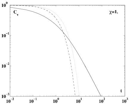
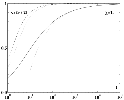
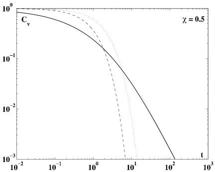
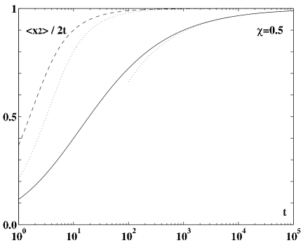
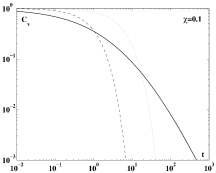
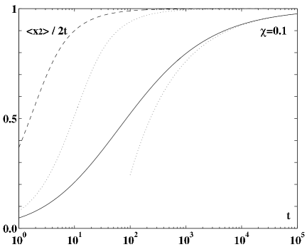
Figure 1: From top to bottom plots on the velocity correlation and on the displacement variance for $\chi=1,0.5,0.1$

We note that in the time interval necessary to reach the asymptotic behaviour the displacement variance exhibits a marked deviation from the standard diffusion. Because this time interval turns out to be orders of magnitude longer than the classical one, it is relevant to discuss about various diffusion regimes before the normal one is established and consequently about the nature of the anomalous diffusion.

In order to explore the nature of the anomalous diffusion we follow the following reasonings. At first, we find it convenient to introduce the instantaneous diffusion coefficient

$$D(t):=\frac{1}{2}\,\frac{d}{dt}{\langle\,X^{2}(t)\,\rangle}\,.$$

We note that such coefficient is suitable to be measured in experiments.

If we assume that ${\langle\,X^{2}(t)\,\rangle}$ varies in a range of $t$, say $t_{k}\leq t\leq t_{k+1}$, approximatively as a power law

$${{\langle\,X^{2}(t)\,\rangle}\simeq a\,t^{\alpha_{k}}\,,\quad t_{k}\leq t\leq t_{k+1}\,,}$$

where $a$ is assumed to be a suitable constant of dimensions $L^{2}\,T^{-\alpha}$, called effective diffusion coefficient, we are usually led to say that the diffusion regime is anomalous if $\alpha\neq 1$, precisely

• slow diffusion or sub-diffusion if $\,0<\alpha_{k}<1\,,$

• fast diffusion or super-diffusion if $\,1<\alpha_{k}<2\,.$

When $\alpha_{k}=2$ the diffusion regime is said to be ballistic; and, of course, when $\alpha_{k}=1$ the diffusion is normal.

We easily recognize from Eq. (4.2) that the power $\alpha_{k}$ can be written as

$${\alpha_{k}=\frac{d({\rm log}\,{\langle\,X^{2}(t)\,\rangle)}}{d({\rm log}\,t)},\;\;t_{k}\leq t\leq t_{k+1}.}$$

In fact from (4.2) we get for any $t_{k}\leq t\leq t_{k+1}$

$${\rm log}\,{\langle\,X^{2}(t)\,\rangle}={\rm log}\,\left[a\,t^{\alpha_{k}}\right]={\rm log}\,a+\alpha_{k}\,{\rm log}\,t\Longrightarrow\;(4.3)$$

Then, varying $k$ we are able to define a function $\alpha(t)$, representing a sort of instantaneous diffusion parameter, which expresses, locally, the characterization of the regimes of anomalous diffusion. In the following plots we shall exhibit $\langle\,X^{2}(t)\,\rangle$ as given by (3.22) with $D(t)$ as given by (4.1) and in addition ${\rm log}\,\langle\,X^{2}(t)\,\rangle$ with $\alpha(t)$ as given by (4.3).

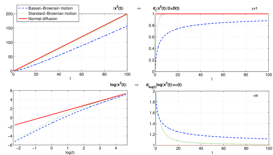
Figure 2: Plots on the displacement variance for $\chi=1$

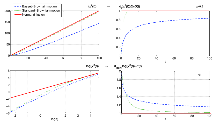
Figure 3: Plots on the displacement variance for $\chi=0.5$

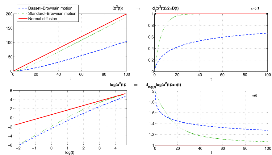
Figure 4: Plots on the displacement variance for $\chi=0.1$

We will note that in all cases $D(t)$ is an increasing function of time, starting from $0$ at $t=0$ and getting $1$ in the limit as $t\to\infty$. On the other hand, $\alpha(t)$ is a decreasing function of time, starting from $2$ at $t=0$ (ballistic regime) and getting $1$ in the limit as $t\to\infty$ (normal diffusion).

In our plots we scale the time $t$ with the equilibrium relaxation $\sigma_{e}$ given by (3.1). and, as usual, we assume for $\chi$ lower and lower values $\chi=1,0.5,0.1$. We easily recognize that the retarding effect of the Basset force is larger for lighter particles, so for them the exponent $\alpha(t)$ remains over 1 for longer times so that, in experiments of limited time duration, this effect could be interpreted as fast diffusion.

5 Conclusions

The velocity autocorrelation and the displacement variance of a Brownian particle moving in an incompressible viscous fluid are known to be the fundamental quantities that characterize the evolution in time of the related stochastic process. Here they are calculated taking into account the effects of added mass and both Stokes and Basset hydrodynamic forces that describe the friction effects, respectively in the steady state and in the transient state of the motion.

The explicit expressions of these quantities versus time are computed and compared with the respective ones for the classical Brownian motion.

The effect of added mass is only to modify the time scale, that is the characteristic relaxation time induced by the Stokes force. The effect of the Basset force, which is of hereditary type namely history-dependent, is to perturb the white noise of the random force and change the decay character of the velocity autocorrelation function from pure exponential to power law because of the presence of functions of Mittag-Leffler type of order 1/2.

Furthermore, the displacement variance is shown to exhibit, for sufficiently long times, the linear behaviour which is typical of normal diffusion, with the same diffusion coefficient of the classical case. However, due to the Mittag-Leffler functions, the Basset history force induces a very long retarding effect in the establishing of the linear behaviour, which could appear, at least for light particles, as a manifestation of anomalous diffusion of the fast type (super-diffusion).

Appendix A

Let us consider the generalized Langevin equation (3.10), that we write as

$$R(t)=m_{e}\,\left[\dot{V}(t)+\,\gamma(t)*V(t)\right]\,,$$

where $\cdot\hbox{}$ denotes time differentiation and $*$ time convolution. The assumption of stationarity for the stochastic processes along with the following hypothesis

$$\langle\,R(t)\,\rangle=0\,,\quad\langle\,V(0)\,R(t)\,\rangle=0\,,\quad t>0\,,$$

allows us to derive, by using the Laplace transforms, the two fluctuation-dissipation theorems

$$\widetilde{C}_{V}(s):=\widetilde{{\langle\,V(0)\,V(t)\,\rangle}}=\frac{\langle\,V^{2}(0)\,\rangle}{s+\widetilde{\gamma}(s)}\,,$$

and

$$\widetilde{C}_{R}(s):=\widetilde{{\langle\,R(0)\,R(t)\,\rangle}}=m_{e}^{2}\,{\langle\,V^{2}(0)\,\rangle}\,\widetilde{\gamma}(s)\,.$$

Our derivation is alternative to the original one by Kubo (1966) [43] who used Fourier transforms; furthermore, it appears useful for the treatment of our fractional Langevin equation.

Multiplying both sides of (A.1) by $V(0)$ and averaging, we obtain

$${\langle\,V(0)\,\dot{V}(t)\,\rangle}+\,\gamma(t)*{\langle\,V(0)\,V(t)\,\rangle}=0\,.$$

The application of the Laplace transform to both sides of (A.5) yields

$$s\,\widetilde{{\langle\,V(0)\,V(t)\,\rangle}}\,-\,{\langle\,V^{2}(0)\,\rangle}\,+\,\widetilde{\gamma}(s)\,\widetilde{{\langle\,V(0)\,V(t)\,\rangle}}=0\,,$$

from which we just obtain (A.3).

Multiplying both sides of (A.1) by $R(0)$ and averaging, we obtain

$$C_{R}(t):={\langle\,R(0)\,R(t)\,\rangle}=m_{e}^{2}\,\left[{\langle\,\dot{V}(0)\,\dot{V}(t)\,\rangle}+\,\gamma(t)*{\langle\,\dot{V}(0)\,V(t)\,\rangle}\,\right]\,.$$

Multiplying both sides of (A.1) by $R(0)$ and averaging, we obtain

$$C_{R}(t):={\langle\,R(0)\,R(t)\,\rangle}=m_{e}^{2}\,\left[{\langle\,\dot{V}(0)\,\dot{V}(t)\,\rangle}+\,\gamma(t)*{\langle\,\dot{V}(0)\,V(t)\,\rangle}\,\right]\,.$$

Noting that, by the stationary condition,

$${\langle\,\dot{V}(0)\,V(0)\,\rangle}=0\,,\quad{\langle\,\dot{V}(0)\,V(t)\,\rangle}=-\,{\langle\,V(0)\,\dot{V}(t)\,\rangle}\,,$$

the application of the Laplace transform to both sides of (A.7) yields

$$\widetilde{C}_{R}(s)=m_{e}^{2}\,\left\{s\,\widetilde{{\langle\,\dot{V}(0)\,V(t)\,\rangle}}-\widetilde{\gamma}(s)\,\left[s\,\widetilde{{\langle\,V(0)\,V(t)\,\rangle}}-{\langle\,V^{2}(0)\,\rangle}\right]\right\}\,.$$

Since

$$\widetilde{{\langle\,\dot{V}(0)\,V(t)\,\rangle}}=-\,\widetilde{{\langle\,V(0)\,\dot{V}(t)\,\rangle}}=-s\,\widetilde{{\langle\,V(0)\,V(t)\,\rangle}}+{\langle\,V^{2}(0)\,\rangle}\,,$$

we get

$$\widetilde{C}_{R}(s)=m_{e}^{2}\,\left\{s\,\left[-s\,\widetilde{C}_{V}(s)+{\langle\,V^{2}(0)\,\rangle}-\widetilde{\gamma}(s)\,\widetilde{C}_{V}(s)\,\right]+\widetilde{\gamma}(s)\,{\langle\,V^{2}(0)\,\rangle}\right\}\,,$$

from which, accounting for (A.3), we just obtain (A.4).

Appendix B

In this Appendix we report the detailed manipulations necessary to obtain the result (3.19) as Laplace inversion of (3.15). For this purpose we need to consider the Laplace transform

$$\widetilde{N}(s)={\frac{1}{s+b\,{s}^{1/2}+1}}\,,\quad b=\sqrt{\beta}\,,$$

and recognize that

$$\frac{C_{V}(t)}{{\langle\,V^{2}(0)\,\rangle}}=N(t/\sigma_{e})\,\div\,\sigma_{e}\,\widetilde{N}(\sigma_{e}\,s)=\frac{1}{s+\sqrt{\beta/\sigma_{e}}\,s^{1/2}+1/\sigma_{e}}\,,$$

where we have used the sign $\div$ for the juxtaposition of a function depending on $t$ with its Laplace transform depending on $s\,.$ The required result is obtained by expanding $\widetilde{N}(s)$ into partial fractions and then inverting. Considering the two roots $\lambda_{\pm}$ of the polynomial $P(z)\equiv z^{2}+b\,z+1\,$ with $z=s^{1/2}\,,$ we must treat separately the following two cases: $i)\;\;0<b<2\,,\quad{\rm or}\quad 2<b<3\,,$ and $ii)\;\;b=2\,,$ which correspond to two distinct roots ($\lambda_{+}\neq\lambda_{-}$), or two coincident roots ($\lambda_{+}\equiv\lambda_{-}=-1$), respectively. We obtain

$i)\quad b\neq 2\,\Longleftrightarrow\,\beta\neq 4\,,\;\chi\neq 5/8\,,$

$$\widetilde{N}(s)=\frac{1}{s+b\,{s}^{1/2}+1}=\frac{A_{+}}{{s}^{1/2}\,({s}^{1/2}-\lambda_{+})}-\frac{A_{-}}{{s}^{1/2}\,({s}^{1/2}-\lambda_{-})}\,,$$

with

$$\lambda_{\pm}=\frac{-b\pm(b^{2}-4)^{1/2}}{2}=\frac{1}{\lambda_{\mp}}\,,\quad A_{\pm}=\frac{\lambda_{\pm}}{\lambda_{+}-\lambda_{-}}\,;$$

$ii)\quad b=2\,\Longleftrightarrow\,\beta=4\,,\;\chi=5/8\,,$

$$\widetilde{N}(s)=\frac{1}{s+2\,{s}^{1/2}+1}=\frac{1}{({s}^{1/2}+1)^{2}}\,.$$

The Laplace inversion of (B.3) and (B.5) turns out, see below,

$$N(t)=\left\{\begin{array}[]{ll}i)&A_{+}\,E_{1/2}(\lambda_{+}\sqrt{t})-A_{-}E_{1/2}(\lambda_{-}\sqrt{t}),\\ ii)&(1+2t)\,E_{1/2}\,(-\sqrt{t})-2\,\sqrt{t/\pi}\end{array}\right.$$

where

$$E_{1/2}(\lambda\,\sqrt{t})=\sum_{n=0}^{\infty}\frac{\lambda^{n}\,t^{n/2}}{\Gamma(n/2+1)}={\rm e}^{\displaystyle\lambda^{2}\,t}\,{\rm erfc}(-\lambda\,\sqrt{t})$$

denotes the Mittag-Leffler function of order $1/2\,$ and erfc denotes the complementary error function. In view of (B.1-2), equation (B.6) is equivalent to (3.19).

Let us first recall the essentials of the generic Mittag-Leffler function in the framework of the Laplace transforms. The Mittag-Leffler function $E_{\alpha}(z)$ with $\alpha>0\,,$ so named from the great Swedish mathematician who introduced it at the beginning of this century, is defined by the following series representation, valid in the whole complex plane,

$$E_{\alpha}(z)=\sum_{n=0}^{\infty}\frac{z^{n}}{\Gamma(\alpha n+1)}\,,\quad\alpha>0\,,\quad z\in{\rm C\hskip-4.8pt\vrule height=6.0pt,width=0.1831pt\hskip 5.0pt}\,.$$

It turns out that $E_{\alpha}(z)$ is an entire function, of order $\rho=1/\alpha\,$ and type $1\,,$ which provides a generalization of the exponential function.

The Mittag-Leffler function is connected to the Laplace integral through the equation

$$\int_{0}^{\infty}\!\!\!{\rm e}^{-u}\,E_{\alpha}\left(u^{\alpha}\,z\right)\,du=\frac{1}{1-z}\,,\quad\alpha>0\,.$$

This integral is fundamental in the evaluation of the Laplace transform of $E_{\alpha}\left(\lambda\,t^{\alpha}\right)$ with $\lambda\in{\rm C\hskip-4.8pt\vrule height=6.0pt,width=0.1831pt\hskip 5.0pt}\,$ and $t\geq 0\,.$ Putting in (B.9) $u=st$ and $u^{\alpha}\,z=\lambda\,t^{\alpha}\,,$ we get the following Laplace transform pair

$$E_{\alpha}\left(\lambda\,t^{\alpha}\right)\div\frac{s^{\alpha-1}}{s^{\alpha}-\lambda}\,,\quad Re\,s>|\lambda|^{1/\alpha}\,.$$

We note that, up to our knowledge, in the handbooks containing tables for the Laplace transforms, the Mittag-Leffler function is ignored so that the transform pair (B.10) does not appear if not in the special case $\alpha=1/2\,.$ In fact, in this case we recover from (B.10) the basic Laplace transform pair

$$\frac{1}{{s}^{1/2}\,({s}^{1/2}-\lambda)}\,\div\,{E_{1/2}({\lambda\,{\sqrt{t}}})}\,,$$

where the Mittag-Leffler function can be expressed in terms of known functions, as shown in (B.7). As an exercise we can derive from (B.11) the following transform pairs and consequently the result (B.6):

$$\frac{1}{{s}^{1/2}-\lambda}=\frac{1}{{s}^{1/2}}+\frac{\lambda}{{s}^{1/2}\,({s}^{1/2}-\lambda)}\,\div\,\frac{1}{\sqrt{\pi\,t}}+\lambda\,{E_{1/2}({\lambda\,{\sqrt{t}}})}\,,$$

$$\frac{1}{{s}^{1/2}\,({s}^{1/2}-\lambda)^{2}}=-2\,\frac{d}{ds}\,\left(\frac{1}{{s}^{1/2}-\lambda}\right)\,\div\,2\,\sqrt{\frac{t}{\pi}}+2\,\lambda\,t\,{E_{1/2}({\lambda\,{\sqrt{t}}})}\,,$$

$$\begin{array}[]{llll}\displaystyle\frac{1}{({s}^{1/2}-\lambda)^{2}}&\displaystyle=&\displaystyle\frac{1}{{s}^{1/2}\,({s}^{1/2}-\lambda)}+\frac{\lambda}{{s}^{1/2}\,({s}^{1/2}-\lambda)^{2}}\\ &\div&2\lambda\sqrt{\frac{t}{\pi}}+(1+2\,\lambda^{2}\,t)\,{E_{1/2}({\lambda\,{\sqrt{t}}})}\end{array}$$

References

- [1] N.K. Ailwadi and B.J. Berne, Cooperative phenomena and the decay of the angular momentum correlation function, J. Chem. Phys. 54 (1971), 3569–3571.
- [2] B.J. Alder and T.E. Wainwrigh, Decay of velocity autocorrelation function, Phys. Rev. A 1 (1970), 18–21.
- [3] G.K. Batchelor, An Introduction to Fluid Dynamics, Cambridge Univ. Press, Cambridge, 1967.
- [4] A. Bazzani, G. Bassi and G. Turchetti, Diffusion and memory effects for stochastic processes and fractional Langevin equations, Physica A 324 (2003), 530–550.
- [5] D. Bedeaux and P. Mazur, Brownian motion and fluctuating hydrodynamics, Physica 76 (1974), 247–258.
- [6] J.-P. Bouchaud and A. Georges, Anomalous diffusion in disordered media: statistical mechanisms, models and physical applications, Physics Reports 195 (1990), 127–293.
- [7] A.A. Budini and M.O. Cáceres, Functional characterization of generalized Langevin equations, J. Phys. A: Math. Gen. 37 (2004), 5959–5981.
- [8] M. Caputo, Linear models of dissipation whose is almost frequency independent, Part II, Geophys. J. R. Astr. Soc. 13 (1967), 529–539.
- [9] M. Caputo, Elasticità e Dissipazione, Zanichelli, Bologna, 1969. [in Italian]
- [10] M. Caputo and F. Mainardi, Linear models of dissipation in anelastic solids, Riv. Nuovo Cimento (Ser. II) 1 (1971), 161–198.
- [11] A. Carpinteri and F. Mainardi (Editors), Fractals and Fractional Calculus in Continuum Mechanics. Springer Verlag, Wien and New York, 1997.
- [12] K.M. Case, Velocity fluctuations of a body in a fluid, Phys. Fluids, 14 (1971), 2091–2095.
- [13] Y.S. Chow and J.J. Hermans, Effect of inertia on the Brownian motion of rigid particles in a viscous fluid, J. Chem. Phys. 56 (1972-a), 3150–3154.
- [14] Y.S. Chow and J.J. Hermans, Autocorrelation functions for a Brownian particle, J. Chem. Phys. 57 (1972-b) 1799–1800.
- [15] Y.S. Chow and J.J. Hermans, Brownian motion of a spherical particle in a compressible fluid, Physica, 65 (1972-c), 156–162.
- [16] H.J.H. Clercx and P.P.J.M. Schram, Brownian particles in shear flow and harmonic potentials: a study of long-time tails, Phys. Rev. A 46 (1992), 1942–1950.
- [17] W.T. Coffey, Yu.P. Kalmykov and J.T. Waldrom, The Langevin Equation, 2-nd Ed. World Scientific, Singapore 2004
- [18] M.A. Despṕosito and A.D. Viñales, Subdiffusive behavior in a trapping potential: mean square displacement and velocity autocorrelation function, Phys. Rev. E 80 (2009), 021111/1–7
- [19] G. Doetsch, Introduction to the Theory and Application of the Laplace Transformation, Springer Verlag, Berlin, 1974.
- [20] A.A. Dubkov, B. Spagnolo and V.V. Uchaikin, Lévy flight superdiffusion: an introduction, Int. Journal of Bifurcation and Chaos 18 No 9 (2008), 2649–2671.
- [21] J.W. Dufty, Gaussian model for fluctuation of a Brownian particle, Phys. Fluids 17 (1974), 328–333.
- [22] C.H. Eab and S.C. Lim, Fractional generalized Langevin equation approach to single-file diffusion, E-print: http://arxiv.org/abs/0910.4734 (2009), pp. 1-10.
- [23] A. Erdélyi (Ed.), Higher Transcendental Functions, Bateman Project, McGraw-Hill, New York, 1955, Vol. 3, Ch. 18, pp. 206–227.
- [24] K.S. Fa, Generalized Langevin equation with fractional derivative and long–time correlation function, Phys. Rev. E. 73 (2006), 061104/1–4.
- [25] K.S. Fa, Fractional Langevin equation and Riemann-Liouville fractional derivative, Eur. Phys. J. E. 24 (2007), 139–143.
- [26] B.U. Felderhof, On the derivation of the fluctuation-dissipation theorem, J. Phys. A: Math. Gen. 11 (1978), 921–927.
- [27] B.U. Felderhof, Motion of a sphere in a viscous incompressible fluid at low Reynolds number, Physica A, 175 (1991), 114–126.
- [28] R. Figueiredo Camargo, A.O. Chiacchio, R. Charmet and E. Capelas de Oliveira, Solution of the fractional Langevin equation and the Mittag-Leffler functions, J. Math. Phys. 50 (2009), 063507/1–8.
- [29] R. Figueiredo Camargo, E. Capelas de Oliveira and J. Waz Jr, On anomalous diffusion and the fractional generalized Langevin equation for a harmonic oscillator, J. Math. Phys. 50 (2009), 123518/1–13.
- [30] I.M. Gel’fand and G.E. Shilov, Generalized Functions, Vol. 1, Academic Press, New York, 1964.
- [31] M. Giona and H.E. Roman, Fractional diffusion equation for transport phenomena in random media, Physica A, 185 (1992), 82–97.
- [32] R Gorenflo and F. Mainardi, Fractional calculus: integral and differential equations of fractional order, in: A. Carpinteri and F. Mainardi (Eds), Fractals and Fractional Calculus in Continuum Mechanics, Springer Verlag, Wien and New York, 1997, pp. 223–276. E-print: http://arxiv.org/abs/0805.3823
- [33] R. Gorenflo, F. Mainardi, D. Moretti, G. Pagnini, and P. Paradisi, Discrete random walk models for space-time fractional diffusion, Chemical Physics 284 (2002), 521–544. E-print: http://arxiv.org/abs/cond-mat/0702072
- [34] P. Grigolini, A. Rocco and B.J. West, Fractional calculus as a macroscopic manifestation of randomness, Phys. Rev. E 59 (1999), 2603–2613.
- [35] E.H. Hauge and A. Martin-Löf, Fluctuating hydrodynamics and Brownian motion, J. Stat. Phys. 7 (1973), 259–281.
- [36] R. Hilfer (Editor), Applications of Fractional Calculus in Physics, World Scientific, Singapore, 2000.
- [37] E.J. Hinch, Applications of the Langevin equation to fluid suspension, J. Fluid. Mech. 72 (1975), 499–511.
- [38] J.T. Hynes, On Hydrodynamic models for Brownian motion, J. Chem. Phys. 57 (1972), 5612–5613.
- [39] S. Khan and A.M. Reynolds, Derivation of a Fokker-Planck equation for generalized Langevin equation, Physica A 350 (2005), 183-188.
- [40] A.A. Kilbas, H.M. Srivastava and J.J. Trujillo, Theory and Applications of Fractional Differential Equations, Elsevier, Amsterdam, 2006.
- [41] R. Klages, G. Radons and I.M. Sokolov (Editors) Anomalous Transport: Foundations and Applications, Wiley-VCH, Weinheim, Germany, 2008.
- [42] V. Kobolev and E. Romanov, Fractional Langevin equation to describe anomalous diffusion, Progress of Theoretical Physics Suppl. No. 139 (2000), 470–476. E-Print http://arxiv.org/abs/chao-dyn/990800
- [43] R. Kubo, The fluctuation-dissipation theorem, Reports on Progress in Physics 29 (1966), 255–284.
- [44] R. Kubo, M. Toda and N. Hashitsume, Statistical Physics II, Nonequilibrium Statistical Mechanics, Springer Verlag, Berlin, 1991.
- [45] E. Lutz, Fractional Langevin equation, Phys. Rev. E 64 (2001), 051106/1–4.
- [46] F. Mainardi, Fractional relaxation-oscillation and fractional diffusion-wave phenomena, Chaos Solitons and Fractals 7 (1996), 1461–1477.
- [47] F. Mainardi, Fractional calculus: some Bbasic problems in continuum and statistical mechanics, in: A. Carpinteri and F. Mainardi (Eds), Fractals and Fractional Calculus in Continuum Mechanics, Springer Verlag, Wien and New York, 1997, pp. 291–348.
- [48] F. Mainardi and R. Gorenflo, On Mittag-Leffler type functions in fractional evolution processes, J. Comput. & Appl. Mathematics 118 (2000), 283–299.
- [49] F. Mainardi, Yu. Luchko and G. Pagnini, The fundamental solution of the space-time fractional diffusion equation. Fractional Calculus and Applied Analysis 4 (2001), 153–192. E-print: http://arxiv.org/abs/cond-mat/0702419
- [50] F. Mainardi and P. Pironi, ”The Fractional Langevin Equation: the Brownian Motion Revisited”, Extracta Mathematicae 11 (1996) 140-154. E-print http://arxiv.org/abs/0806.1010
- [51] F. Mainardi, P. Pironi and F. Tampieri, On a generalization of the Basset problem via fractional calculus, in: B. Tabarrok and S. Dost (Eds), Proceedings CANCAM 95, University of Victoria, Canada, 1995, Vol. 2, pp. 836–837.
- [52] M.R. Maxey and J.J. Riley, Equation of motion for a small rigid sphere in a nonuniform flow, Phys. Fluids 26 (1983), 883–889.
- [53] R.M. Mazo, Theory of Brownian motion. IV. A hydrodynamic model for the friction factor, J. Chem. Phys. 54 (1971), 3712–3713.
- [54] M.M. Meerschaert, D.A. Benson, H.-P. Scheffler and B. Baeumer, Stochastic solutions of space fractional diffusion equation, Phys. Rev. E 65 (2002), 041103-1/4.
- [55] R. Metzler and J. Klafter, Subdiffusive transport close to thermal equilibrium: from the Langevin equation to fractional diffusion, Phys. Rev. E 61 (2000), 6308–6311.
- [56] R. Metzler and J. Klafter, The random walk’s guide to anomalous diffusion: a fractional dynamics approach, Phys. Reports 339 (2000), 1–77..
- [57] R. Metzler and J. Klafter, The restaurant at the end of the random walk: Recent developments in the description of anomalous transport by fractional dynamics, J. Phys. A. Math. Gen. 37 (2004), R161–R208 .
- [58] K.S. Miller and B. Ross, An Introduction to the Fractional Calculus and Fractional Differential Equations, Wiley, New-York, 1993.
- [59] R. Muralidhar, D. Ramkrishna, H. Nakanishi and D.J. Jacobs, Anomalous diffusion: a dynamic perspective, Physica A 167 (1990), 539–559.
- [60] M. Nelkin, Inertial effects in motion driven by hydrodynamic fluctuations, Phys. Fluids 15 (1972), 1685–1690.
- [61] K.B. Oldham and J. Spanier, The Fractional Calculus, Academic Press, New York, 1974.
- [62] G.L. Paul and P.N. Pusey, Observation of a long-time tail in Brownian motion, J. Phys. A: Math. Gen. 14 (1981), 3301–3327.
- [63] A. Piryatinska, A.I. Saichev and W.A. Woyczynski, Models of anomalous diffusion: the subdiffusive case, Physica A 349 (2005), 375–420.
- [64] I. Podlubny, Fractional Differential Equations, Academic Press, San Diego, 1999.
- [65] Y. Pomeau and P. Résibois, Time dependent correlation functions and mode-mode coupling theories, Physics Reports 19 (1975), 63–139.
- [66] J.M. Porrà, K.G. Wong and J. Masoliver, generalized Langevin equations: anomalous diffusion and probability distributions, Phys. Rev. E 53 (1996), 5872–5881.
- [67] N. Pottier and A. Mauger, Anomalous diffusion of a particle in an aging medium, Physica A 332 (2004), 15–28.
- [68] L.E. Reichl, Translation Brownian motion in a fluid with internal degrees of freedom, Phys. Rev. 24 (1981), 1609–1616.
- [69] B. Ross (Ed.), Fractional Calculus and its Applications, Springer-Verlag, Berlin, 1975. [Lecture Notes in Mathematics No. 457]
- [70] A.I Saichev and S.G. Utkin Models of fractional diffusion (in Russian), Modern Problems in Statistical Physics 2 No 1 (2002), 5–43.
- [71] A.I. Saichev and G.M. Zaslavsky, Fractional kinetic equations: solutions and applications. Chaos 7 (1997), 753–764.
- [72] S.G. Samko, A.A. Kilbas and O.I. Marichev, Fractional Integrals and Derivatives, Theory and Applications, Gordon and Breach, Amsterdam, 1993. [Engl. Transl. from the Russian, Integrals and Derivatives of Fractional Order and Some of their Applications, Nauka i Tekhnika, Minsk, 1987]
- [73] A. Taloni and M.A. Lomholt, Langevin formulation for single-file diffusion, Phys. Rev. E 78 (2008), 051116/1–8.
- [74] V.V. Uchaikin Method of fractional derivatives, ArteShock-Press, Uljanovsk, 2008, in Russian.
- [75] V.V. Uchaikin, V.M. Zolotarev, Chance and Stability: stable laws and their application, VSP [Modern Probability and Statistics], Utrecht, 1999.
- [76] A.D. Viñales and M.A Despósito, Anomalous diffusion: exact solution of the generalized Langevin equation for harmonically bounded particle, Phys. Rev. E. 73 (2006), 016111/1-4
- [77] A.D. Viñales and M.A Despósito, Anomalous diffusion induced by a Mittag-Leffler correlated noise, Phys. Rev. E. 75 (2007), 042102/1-4
- [78] A.D. Viñales, K.G. Wang and M.A Despósito, Anomalous diffusion behavior of a harmonic oscillator driven by a Mittag-Leffler noise, Phys. Rev. E. 80 (2009), 011101/1-6
- [79] K.C. Wang, Long-time correlation effects and biased anomalous diffusion, Phys. Rev. A 45 (1992), 833–837.
- [80] K.C. Wang and C.W. Lung, Long-time correlation effects and fractal Brownian motion, Phys. Lett. A 151 (1990), 119–121.
- [81] K.C. Wang and M. Tokuyama, Nonequilibrium statistical description of anomalous diffusion, Physica A 265 (1999), 341–351.
- [82] M. Warner, The long-time fluctuations of a Brownian sphere, J. Phys. A: Math. Gen. 12 (1979), 1511–1519.
- [83] A. Widom, Velocity fluctuations of a hard-core Brownian particle, Phys. Rev. A 3 (1971), 1394–1396.
- [84] A.H. Zemanian, Distribution Theory and Transform Analysis, McGraw-Hill, New York, 1965.
- [85] R. Zwanzig and M. Bixon, Hydrodynamic theory of the velocity correlation function, Phys. Rev. A 2 (1970), 2005-2012.
- [86] R. Zwanzig and M. Bixon, Compressibility effects in the hydrodynamic theory of Brownian motion, J. Fluid Mech. 69 (1975), 21–25.