XMM-Newton  and SUZAKU  detection of an X-ray emitting shell around the pulsar wind nebula G54.1+0.3

Abstract

Context. Recent X-ray observations have proved to be very effective in detecting previously unknown supernova remnant shells around pulsar wind nebulae (PWNe), and in these cases the characteristics of the shell provide further clues on the evolutionary stage of the embedded PWN. However, it is not clear why some PWNe are still “naked”.

Aims. We carried out an X-ray observational campaign targeted at the PWN G54.1+0.3, the “close cousin” of the Crab, with the aim to detect the associated SNR shell.

Methods. We analyzed an XMM-Newton and Suzaku observations of G54.1+0.3  and we model out the contribution of dust scattering halo.

Results. We detected an intrinsic faint diffuse X-ray emission surrounding the PWN up to $\sim 6\hbox{${}^{\prime}$}$ ($\sim 10$ pc) from the pulsar, characterized by a hard spectrum, which can be modeled either with a power-law ($\gamma=2.9$) or with a thermal plasma model ($kT=2.0$ keV.)

Conclusions. If the shell is thermal, we derive an explosion energy $E=0.5-1.6\times 10^{51}$ erg, a pre-shock ISM density of 0.2 cm^-3 and an age of $\sim 2000$ yr. Using these results in the MHD model of PWN-SNR evolution, we obtain an excellent agreement between the predicted and observed location of the shell and PWN shock.

1 Introduction

One of the most intriguing problems in the field of the Pulsar Wind Nebulae (PWNe) study is the lack of a shell around some of these objects. This is somehow disturbing for the consolidated picture of a remnant of a core-collapse supernova, which indicates that the PWN is expanding inside the host supernova remnant, giving rise to a variety of complex phenomena, like reverberation, Rayleigh-Taylor instability at the interface between the PWN and ejecta, rejuvenating the shell, etc. (e.g. van der Swaluw et al. 2001; Blondin et al. 2001; Chevalier 2005; Gelfand et al. 2009 and references therein). One of the reasons could be the lack of deep observations aimed at the PWN surroundings. Indeed, recently a shell-like component has been observed in many objects, such as G21.5–0.9 (Bandiera & Bocchino 2004; Bocchino et al. 2005), G0.9+0.1 (Porquet et al. 2003), 3C58 (Bocchino et al. 2001; Gotthelf et al. 2007). Therefore, X-ray observations are very effective for the discovery of associated shell components, even in the presence of high absorption column densities (G21.5–0.9 has $N_{H}\sim 2\times 10^{22}{\,\rm cm^{-2}}$; G0.9+0.1 even $\sim 10^{23}{\,\rm cm^{-2}}$).

The objects in which pulsar, plerion, and shell are all detected (collectively known as composite SNRs) are extremely important to set the physical conditions for their modeling. The properties and the evolution of a PWN are determined by the interaction of the pulsar wind with the ambient medium. The effectiveness by which the surrounding matter confines the PWN is very important to determine the the level of the synchrotron emission from the nebula. Therefore, measuring density and pressure in the shell component is needed for better constraining the models of the PWN. Moreover, the pulsar, the PWN and the shell would allow us to estimate in independent ways some quantities, such as the actual age of the object, or the internal pressure of the nebula. This redundancy would allow us also to verify our assumptions, like that on the level of equipartition in the PWN and that on how reliable is the age estimated from the pulsar spin-down properties.

G54.1+0.3  is the Galactic PWN that most closely resembles the Crab Nebula: this is the reason why Lu et al. (2002) have dubbed it “a close cousin of the Crab Nebula”. Using Chandra data, Lu et al. (2002) have shown the presence of a well defined torus of $\sim 10^{\prime\prime}$ in diameter, together with elongations, toward E and W directions, which could be ascribed to X-ray jets. From those data, the size of the X-ray nebula appears $\sim 1^{\prime}$, but the outer part of the nebula is very faint, and its edge is poorly defined. At radio wavelengths, instead, the nebular size is $\sim 1.5^{\prime}$ (Velusamy & Becker 1988), corresponding to $\sim 2.7\,d_{6.2}$ pc where $d_{6.2}$ is the distance of G54.1+0.3 in units of that estimated by Leahy et al. (2008), namely $d_{6.2}=d/6.2^{+1.0}_{-0.6}$ kpc. It is important to understand to which extent this difference in size is real (i.e. due to synchrotron losses of the emitting electrons), or it is an artifact of the limited X-ray sensitivity.

Radio maps show a rather amorphous structure, but the radio emission from G54.1+0.3 is highly polarized, up to 20–30% (Velusamy & Becker 1988), and this indicates (similarly to the case of the Crab Nebula) that the nebular field is highly ordered. The X-ray spectrum is a power law with a photon index $-1.9$, an absorption column density $N_{H}\sim 1.6\times 10^{22}{\,\rm cm^{-2}}$ and an X-ray luminosity $L_{X}\sim 1.3\times 10^{33}d_{6.2}^{2}{\,\rm erg\,s^{-1}}$. Camilo et al. (2002) have detected the pulsar PSR J1930+1852 at the center of the nebula, which has a period of 136 ms, a characteristic age of 2900 yr and a spin-down luminosity of $1.2\times 10^{37}$ erg s^-1.

Recently, G54.1+0.3  has attracted some interest because Koo et al. (2008) have identified an IR shell surrounding the PWN at a distance of $\sim 1.5^{\prime}$ from the pulsar. The shell contains a dozen of IR compact sources. Koo et al. (2008) suggests that the sources are young stellar objects, whose formation has been triggered by the wind of the progenitor of the SN. This intriguing possibility has been questioned by Temim et al. (2010), who pointed out that the IR shell may be ejecta dust, rather than a pre-existing ISM dense cloud. Leahy et al. (2008) reported the presence of a molecular cloud partially interacting with the PWN, on the basis of the CO emission around the nebula. Therefore, even if there is no hint of a radio shell around this PWN, there are a number of evidences for interaction between the PWN and the surroundings, so it is worth searching for an X-ray shell.

In Sect. 2 we present a deep X-ray campaign aimed to this PWN, which led to the detection of such a shell. In Sect. 3 we estimate the contribution of the dust scattering halo, showing that it is negligible at the shell location, and in Sect. 4 we discuss our findings comparing them to a PWN-SNR evolution model.

2 Deep XMM-Newton  and SUZAKU  observations

Table 1: X-ray observations used in this work

Satellite	ID	$T_{exp}$ (ks)	Obs. date
XMM-Newton	0406730101	41	26.09.2006
SUZAKU	502077010	84	30.10.2007

We have observed the PWN G54.1+0.3  with XMM-Newton (Jansen et al. 2001) and SUZAKU  (Mitsuda et al. 2007) in 2006 and 2007 respectively. Table 1 summarizes the observations used in this work. The data have been analyzed with the latest software available, namely SAS v8.0 for XMM-Newton and the pipeline v.2.1.6 with HEASOFT v6.6 for SUZAKU. The XMM-Newton data have been screened for proton flares using the sigma clipping algorithm described in Snowden & Kuntz (2007), while for SUZAKU  we have used the standard screening. The image of G54.1+0.3  obtained with the EPIC PN and MOS CCD cameras of XMM-Newton  (Turner et al. 2001; Strüder et al. 2001, with a resolution of $8^{\prime\prime}$ HPD) and the XIS CCD camera of SUZAKU (Koyama et al. 2007, $110^{\prime\prime}$ FWHM) are shown in Fig. 1, in the upper and lower panel respectively.

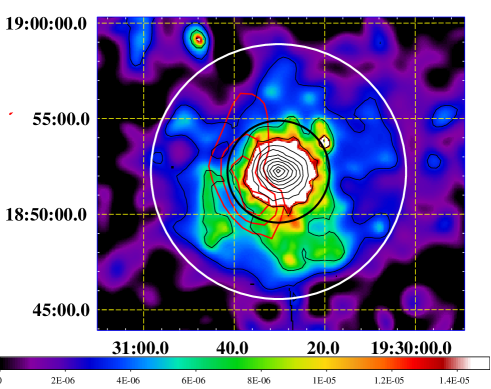
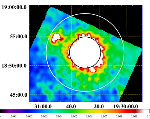
Figure 1: Top panel: XMM-Newton  EPIC  image in the 1–7 keV energy band. The image is a mosaic of background subtracted and vignetting corrected images obtained with the PN, MOS1 and MOS2 cameras. The color scale has been chosen to maximize the visibility of the faint diffuse emission around the bright PWN. The inner (black) circle has a radius of $160^{\prime\prime}$ and includes the extension of the radio plerion, while the outer (white) circle has a radius of 400” and is drawn to guide the eye on the extension of the shell. Black thin contours marks an increase of factor 2 in surface brightness from $3\times 10^{-6}$ to $3.2\times 10^{-3}$ cnt s^-1 pix^-1, where 1 pixel is $4^{\prime\prime}\times 4^{\prime\prime}$. Red contours are drawn form the map of the 53 km s^-1 CO emission published in Fig. 3b of Leahy et al. (2008), and represent a molecular cloud possibly interacting with the PWN. Bottom panel: SUZAKU  image in the 1–7 keV energy band. The image is a mosaic of background subtracted and vignetting corrected images obtained with the XIS0, XIS2 and XIS3. The field of view and circles are the same as in the top panel.

There is a diffuse extended emission surrounding the bright plerion in both images. This diffuse emission seems to have spatial structures as small as $1\hbox{${}^{\prime}$}$. The contrast of surface brightness between the diffuse emission and the core of the PWN is about 1000.

Table 2: SUZAKU  spectral fitting results

Model	$N_{H}$	kT or $\gamma$	$\chi^{2}/dof$
	$10^{22}$ cm-2	keV
Core of the PWN
Power-law	$1.57\pm 0.06$	$1.82\pm 0.04$	925/1145
Shell
Power-law	1.57	$2.9\pm 0.3$	173/215
Thermal	1.57	$2.0\pm 0.4$	196/215

We investigated the nature of the X-ray faint diffuse emission by studying its spectrum both with XMM-Newton  and SUZAKU. For the spectral analysis purposes, we defined a core region and a shell region. The core region is a circle centered on the pulsar with a radius of $160\hbox{${}^{\prime\prime}$}$. This includes all the regions occupied by the radio nebula and its X-ray emission is dominated by the synchrotron emission coming form the PWN. The shell region is an annulus with a inner radius equal to the radius of the core region and an outer radius of $400\hbox{${}^{\prime\prime}$}$. We estimated that the contribution of the core emission in the shell region is 25% for SUZAKU and 1% for XMM-Newton, purely due to the instrumental PSF wings and excluding the additional contribution of dust scattered X-rays. In the case of XMM-Newton, the shell region was further reduced to a pie sector between polar angles $90^{\circ}$ and $135^{\circ}$ (from N, anti-clockwise, where most of the knots are located. The background was taken from the same chip for SUZAKU, while in the case of XMM-Newton we have used both blank fields and the same observation to collect background (in the latter case an annular region with $R_{min}=400\hbox{${}^{\prime\prime}$}$ and $R_{max}=450\hbox{${}^{\prime\prime}$}$ was used), verifying that the results did not change with the particular choice of the background. We fitted the core region, finding that a power-law model describes the data very well. Therefore, we fitted the shell region using a combination of the power-law model used in the core (with parameters fixed to their best-fit core values, including interstellar absorption) and an additional component, chosen among a thermal and a non-thermal model. The core model was used (and rescaled) in the shell region to take into account possible contamination from dust-scattering and from instrumental Point Spread Function. The SUZAKU  results are summarized in Table 2, and seem to indicate that the shell emission which can be modeled either with a thermal component or with a non-thermal power law in the shell spectrum. XMM-Newton gives similar results. The SUZAKU spectrum of the core and the shell are reported in Fig. 2 along with their best-fit models. The core is also detected between 15 and 25 keV using the non-imaging SUZAKU Hard X-ray Detector (HXD) silicon PIN diodes (spectrum also reported in Fig. 2, upper panel), with a flux of $\sim 4\times 10^{-12}$ erg cm^-2 s^-1 in this band. The normalization constant between the PIN and the XIS CCD spectra is $1.3(1.0-1.6)$, a range which includes the expected value of 1.15 (Kokubun et al. 2007).

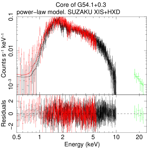
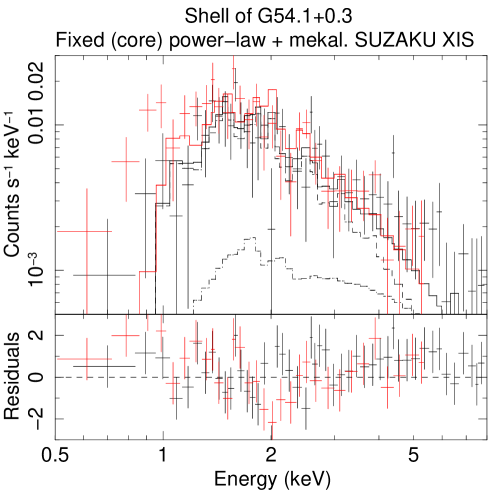
Figure 2: Top: SUZAKU  spectrum of the core region and the best-fit model. XIS0+3, XIS2 and HXD spectra are shown. Bottom: SUZAKU XIS0+3 and XIS2 spectra of the shell region. The total best fit thermal + residual non-thermal component from the core is overplotted, as long as the individual components (dashed).

3 Removal of dust-scattering halo

The presence of a foreground medium may affect in more ways the observed emission from an X-ray source. The best modeled effect is photoelectric absorption, but also dust scattering of the X-ray photons may be important. Its produces an apparent halo around the intrinsic source, which is more prominent at lower energies and may hamper considerably both spectral mapping analysis of diffuse sources and searches of faint surrounding features. Scattering halos may be relevant whenever the column density of the intervening material ($N_{H}$) is high. $N_{H}$ may be derived by fitting the photoelectric absorption of the X-ray spectrum, while the scattering optical depth ($\tau_{\mathrm{sca}}$, estimated at a reference photon energy of 1 keV) by fitting the halo. Predehl & Schmitt (1995) show that the linear regression

$$\tau_{\mathrm{sca}}(1{\,\rm keV})=0.05(N_{H}/10^{21}{\,\rm cm^{-2}})-0.083$$ (1)

can be drawn between these two quantities. For the measured value of $1.57\times 10^{22}{\,\rm cm^{-2}}$ for G54.1+0.3, this relation predicts $\tau_{\mathrm{sca}}(1{\,\rm keV})\simeq 0.7$. This value is however only approximate, because the properties of the dust may be different along different directions, while for the exact value a direct analysis of the halo is required.

While halos of strong, point-like X-ray sources are selected to investigate properties of the dust grains, in this case we have to deal with a fainter, diffuse intrinsic source and therefore the modeling of the halo is necessarily less accurate. On the other hand, our goal here is simply to find a modeling that can subtract efficiently the halo component, without pretending to infer reliable physical properties of the dust distribution.

In the case of a point-like source, we can describe the halo with the following function:

$$I_{\mathrm{sca}}(\theta,E)=F(E)\left(1-\exp(-\tau_{\mathrm{sca}}(E)\right)H(\theta,E).$$ (2)

where $F(E)$ is the source intrinsic flux and $H(\theta,E)$ is a function that we derive and describe in detail in the Appendix A, where we also summarize the basic modeling of a halo and the related assumptions.

In our case, however, the intrinsic source is spatially resolved, and in principle we should convolve the halo for a point-like source with the surface brightness distribution of the actual intrinsic source, in a way to obtain the observed map. This is in general a very complex and numerically heavy task. Moreover, if just one energy band is considered, the number of possible solutions would even be infinite. To solve the problem of separating intrinsic source and halo, one must then carry on a combined fit on radial profiles at different energies, by taking advantage of the known energy dependence of the halo properties. In order to model the energy dependence of the scattering halo, we have produced for each instrument 4 images, in the following spectral bands: 1.0–1.75 keV, 1.75–2.5 keV, 2.5–3.9 keV, and 3.9–7.25 keV. The spectral boundaries have been chosen to get similar numbers of photons in the various bands, with the further constraint of excluding photons softer than 1 keV, for which the simple Rayleigh-Gans scalings with the photon energy (namely optical depth $\propto E^{-2}$ and halo size $\propto E^{-1}$) are no longer valid. The reference energies of the four bands are 1.4, 2.05, 3.07, and 4.94 keV respectively, and are obtained averaging the energies of all photons collected in each band.

Since the intrinsic source is centrally peaked and more concentrated than the halo, and the wings of XMM-Newton PSF are narrower than the observed radial profile, we have applied a simplified approach, by approximating the halo with that for a point-like source. For our final fits we have used only 2 free parameters to model the halo, namely $\tau_{\mathrm{sca}}(1{\,\rm keV})$ and $\theta_{\mathrm{scal}}(1{\,\rm keV})$. Before then, we had attempted also fits using a larger number of parameters, but with the moderate statistics of our data we have found: i. a partial degeneracy between power-law index of the grain size distribution ($q$) and the spatial scale ($\theta_{\mathrm{scal}}$), and therefore we have chosen a rather usual value for $q$ (3.5, see e.g. Predehl & Schmitt 1995); ii. our fits were typically consistent with a wide spread of $z$ (i.e. the position along the line of sight, normalized to the source distance), and therefore we have decided to assume a homogeneous distribution of dust along the line of sight ($z_{\mathrm{min}}=0$ and $z_{\mathrm{max}}=1$). All quantities cited here are described in the Appendix A.

For the intrinsic source we have chosen the following modeling:

$$I_{\mathrm{intr}}(\theta,E)=\frac{F(E)}{C}\left(\exp\left(-\frac{\theta^{2}}{\sigma_{1}^{2}}\right)+A\left(1+\frac{\theta^{2}}{\sigma_{2}^{2}}\right)^{-\alpha_{2}}\right),$$ (3)

where $C=2\sigma_{1}^{2}+A\sigma_{2}^{2}/(\pi(\alpha_{2}-1))$ is the normalization factor. The fitted shape is indeed a convolution of the actual source with the instrumental PSF, but at this level we do not need to separate them. In addition, we have assumed that this shape is independent of $E$: indeed, it is known that the X-ray size of PWNe is slightly decreasing for increasing $E$, but this is only a minor effect, which we cannot adequately describe with the available data, and on the other hand does not affect considerably the results of our fits.

From each image we have extracted a logarithmically spaced radial profile. In order to minimize the statistical noise, the flux values are averaged over several points. In the case of MOS1, due to the absence of the damaged CCD#6, data are missing for a region that is relevant to our purposes, so we use MOS2 only. By analyzing the emission at distances larger than $300\hbox{${}^{\prime\prime}$}$ from the source center, we have estimated the MOS2 background levels for the 4 bands, as about $10^{-4}$ times the surface brightness in the brightest areas. Therefore, we did not apply any correction of the background. With this, we are confident that our profiles are usable over a dynamical range close to $10^{4}$.

Table 3: X-ray dust scattering halo best-fit parameters for G54.1+0.3

Name	$0^{\prime\prime}-120^{\prime\prime}$	$0^{\prime\prime}-200^{\prime\prime}$
$\sigma_{1}$	6.8′′	6.6′′
$A$	0.87	0.97
$\sigma_{2}$	30.7′′	29.2′′
$\alpha_{2}$	2.27	2.22
$\tau_{\mathrm{sca}}(1{\,\rm keV})$	1.15	1.09
$\theta_{\mathrm{scal}}(1{\,\rm keV})$	15.1′	10.2′

For the fits, we have used at first only the inner $120\hbox{${}^{\prime\prime}$}$ of the radial profiles. This to allow an unbiased analysis of structures that may appear at larger radii. However, we also present the results obtained in the inner $200^{\prime\prime}$ of the radial profiles. The results of the fits are presented in Table 3. The results are in general rather similar between different choice of maximum fitting radius.

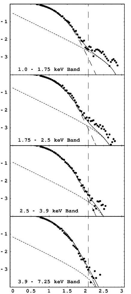
Figure 3: X-ray normalized profiles in the bands 1.0–1.75, 1.75–2.5, 2.5–3.9, and 3.9–7.25 keV of G54.1+0.3  as seen by MOS2 camera of XMM-Newton EPIC. In the x-axis we report the logarithmic distance from the center in arcsec. We have overplotted the best fit halo model, with individual components (intrinsic source, long-dashed line, and halo, short-dashed line). The radial range of the fit extends only to $120\hbox{${}^{\prime\prime}$}$ (the position of the vertical dashed line). See the text for further details on the model. The residuals between $160\hbox{${}^{\prime\prime}$}$ and $400\hbox{${}^{\prime\prime}$}$ (2.2 to 2.6 in logarithmic scale) with respect to the extrapolation of the halo model are due to the X-ray shell.

Fig.  3 shows, the combined MOS2 fits on the 4 bands (for a maximum fitting radius of $120\hbox{${}^{\prime\prime}$}$ marked by the vertical dashed line) and the extrapolation of the best-fit profiles to larger radial distances, compared to the observed profiles. The observed radial profile shows an excess of emission at distances from the center $>100^{\prime\prime}$ which cannot be explained by the dust-scattering halo. If we normalize to the fluxes due to the source plus the halo in the $0^{\prime\prime}-160^{\prime\prime}$ region, the model predicts that the flux due to the halo in the outer $160^{\prime\prime}-400^{\prime\prime}$ annulus are 0.20, 0.10, 0.04 and 0.01 in the 1.0–1.75, 1.75-2.5, 2.5–3.9 and 3.9-7.25 keV respectively (the flux of the source is 0.01 in the same region), while the observed values are $0.28\pm 0.01$, $0.14\pm 0.02$, $0.11\pm 0.02$, $0.16\pm 0.03$, significantly higher than the predicted halo model. We therefore conclude that the excess is due to intrinsic emission from the G54.1+0.3  shell.

4 Discussion

We have reported for the first time the detection of a large faint diffuse X-ray emission around the PWN G54.1+0.3. We have seen that this excess cannot be due to the X-ray dust scattering halo, because an accurate modeling of the halo presented in previous section and in the Appendix A shows that the halo model underpredicts the observed emission between $160\hbox{${}^{\prime\prime}$}$ and $400\hbox{${}^{\prime\prime}$}$ from the center, where the shell is observed. This shell emission has an irregular morphology, but can be enclosed at most inside a circle of 5.7 arcmin radius centered on the pulsar position, corresponding to $\sim 10.3\,d_{6.2}$ pc.

We have seen that the halo spectrum can be interpreted as thermal or non-thermal emission. If we interpret it as the long sought thermal emission of the G54.1+0.3  shell, we can derive some interesting quantities related to the remnant evolution by assuming an expansion governed by the Sedov (1959) solution. The best-fit emission measure is $EM=9\times 10^{-11}$ cm^-5, and the best-fit temperature is 2 keV. According to the model of Ghavamian et al. (2007), electrons cannot be heated directly at this temperature by the shock, so the Coulomb heating by the shocked ions must be at work. Using the relations (6)–(10) of Bocchino & Bandiera (2003), and the best-fit emission measure and temperature, we have computed the plot of Fig. 4, which shows all the possible solutions versus the remnant distance. We have specifically taken into account the case in which electrons are not thermalized with ions, by reporting 3 different cases of electron-ion temperatures in Fig. 4, namely $T_{e}/T_{p}=1$ (electron-ion full equilibration), $T_{e}/T_{p}=1/2$ (moderate electron-ion disequilibrium) and $T_{e}/T_{p}=1/10$ (strong disequilibrium, as in other young SNRs, Ghavamian et al. 2007 and references therein). If we use a distance of 6.2 kpc, we find a range of remnant ages between 2500 and 3300 yr for the equipartition case (solid line in Fig. 4), which is in agreement with the more uncertain estimate of the remnant age (1500–6000 yr) given by Camilo et al. (2002). The inferred ISM pre-shock density is $\sim 0.2$ cm^-3 and the swept up mass is between 23 and 32 M_⊙, while the X-ray emitting mass is 15–20 M_⊙. The explosion energy range is $E=3-7\times 10^{50}$ erg. However, if we drop the assumption of equipartition between electron and ions, we find that $E=1.0(0.5-1.6)\times 10^{51}$ erg for a distance of 6.2 kpc when $T_{e}/T_{p}\sim 1/2$. In this case, the derived age is between 1800 and 2400 yr (dotted line in Fig. 4). Lower values of $T_{e}/T_{p}$ (i.e. $\sim 1/10$) are disfavored by relative high explosion energies (dashed line in Fig. 4). We have seen that the XMM spectral fittings suggest a similar temperature to the SUZAKU  values, but a normalization 10 times lower. In this case, the estimate of the ISM density, explosion energy and swept-up mass must be decreases by a factor of 3. A cross-check with the non-radiative SNR model of Truelove & McKee (1999) gives a transition from ejecta-dominated to Sedov phase at 2500 yr, so the remnant is entering in the adiabatic phase. Given the faintness of the diffuse emission, only a deeper X-ray observation would allow us to derive more reliable values of the shell parameters.

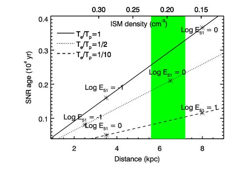
Figure 4: Sedov solutions for the SNR age and distance computed using the X-ray derived parameters of G54.1+0.3  ($kT=2$ keV, SNR radius $6\hbox{${}^{\prime}$}$, emission measure $9\times 10^{11}$ cm^-5). We report 3 different solutions corresponding to full electron-ion equipartition ($T_{e}/T_{p}=1$) and the cases of $T_{e}/T_{p}=1/2$ and $1/10$. The asterisks on the curve mark the corresponding explosion energy of the solutions. The intersection of the curves with the area marked in green (corresponding to the distance estimate of Leahy et al. (2008)) gives the age of the system (for instance, the age is 1800-2400 yr for the case $T_{e}/T_{p}=1/2$, and the energy is $\sim 10^{51}$ erg).

The derived values of density and swept-up mass suggest an expansion in rarefied medium for most of the remnant lifetime. This seems to be in agreement with the findings of Leahy et al. (2008) about the environment of G54.1+0.3. The remnant projected location inside a large IR shell opens up the possibility that G54.1+0.3  have been originated by a SN belonging to the same star cluster whose winds have created the large IR shell. Although the IR shell distance seems to be a little bit larger than the PWN distance (7.2 kpc vs 6.2 kpc), according to Leahy et al. (2008) the uncertainties on the distance do not rule out the association, and the values of the density we derived with the X-ray spectral analysis goes in the same direction. The X-ray shell seems to be larger than the CO cloud reported by Leahy et al. (2008), as shown by the CO contours overplotted in Fig. 1. Koo et al. (2008) showed that G54.1+0.3  has interacted with a star-forming loop located very close to the nebula center (at $\sim 1\hbox{${}^{\prime}$}$ from the pulsar). The loop contains at least 11 young stellar objects (YSOs) which are very bright in the AKARI 15 $\mu$m image of the core of the PWN. Koo et al. (2008) argue that there is no direct evidence for the interaction of the SNR shock with this dense material, so they conclude that the IR loops is a partial shell in a low-density medium and that the SNR shock has propagated well beyond it. This is in agreement with the position of the X-ray shell we have discovered, since we can now compute (using the Truelove & McKee 1999 model) that the shock was at the IR loop position just at 1/10 of the present age. Temim et al. (2010) proposed an explanation in terms of ejecta dust for the IR loop, which is not in contrast with the presence of the X-ray shell.

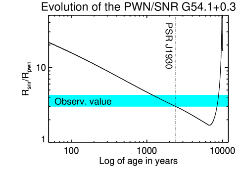
Figure 5: Ratio between the shell radius and PWN radius according to the model of Gelfand et al. (2009), with input parameters tailored to the G54.1+0.3  system (see text for details). The observed value is also reported as a cyan stripe, whose spread is due to the uncertainties in defining the real PWN radius (we have used a minimum of $80\hbox{${}^{\prime\prime}$}$ and a maximum of $114\hbox{${}^{\prime\prime}$}$, on the base of the morphology shown in Fig. 1). The vertical dot-dashed line marks the instant of the run when the simulated pulsar has a characteristic age and spin-down luminosity identical to PSR J1930+1852 as measured by Camilo et al. (2002). In this moment, the model reproduces both the PWN and SNR size and their ratio, strengthening the conclusion that the extended diffuse emission is indeed the SNR shell of the PWN G54.1+0.3.

If the faint diffuse emission we have discovered around the PWN G54.1+0.3 is really the associated SNR shell, then we can compare its properties with the PWN-SNR evolutionary model of Gelfand et al. (2009). This model couples the dynamical and radiative evolution of the PWN with the dynamical properties of the surrounding non-radiative SNR, and predicts several distinctive evolutionary stages, namely the initial expansion, the reverse shock collision, the re-expansion and the second compression. We run the model using as input parameters $E_{sn,51}=1$ and $n_{ism}=0.2$ cm^-3, derived from the best-fit thermal model of the X-ray shell (Fig. 4, $T_{e}/T_{p}=1/2$ case of a moderate deviation from electron-ion equipartition). We assumed an ejecta mass of 8 $M_{\odot}$, and a spin-down timescale of 500 years (close to the value of the Crab; this corresponds to an initial period $P_{0}=56$ ms of the pulsar). The pulsar wind properties are the same as in Table 2 of Gelfand et al. (2009). The resulting dynamical evolution of the shock of the shell and the PWN nebula is shown in Fig. 5, where we plot the ratio between the shell radius and the PWN radius ($R_{snr}/R_{pwn}$) versus time, and a vertical line marks the time when the pulsar has the same characteristic age as measured by Camilo et al. (2002), and its period and period-derivative match what was observed ($\tau_{c}=2900$ yr and a real age of 2400 yr). The predicted $R_{snr}/R_{pwn}$ is remarkably similar to the observed value, and the SNR and PWN sizes (8.7 and 2.8 pc) are in relatively good agreement with observations. According to this model, the PWN has not yet been crushed by the reverse shock (Fig. 5 shows that it will happen at an age of $\sim 7000$ yr, when $R_{snr}/R_{pwn}$ reaches a minimum), in agreement with the lack of sign of crushing, as noted by Temim et al. (2010). We conclude that the thermal parameters we have measured in the faint diffuse emission around the PWN and its size are in good agreement with what we expect from a putative shell of the SNR G54.1+0.3, on the basis of a complete modeling of the SNR-PWN system. We interpret this as a further indication that what we observe is indeed the long sought shell of the remnant.

5 Summary and conclusions

We have analyzed an XMM-Newton  and a SUZAKU  observation of the PWN G54.1+0.3, in the framework of a program aimed to survey the region around this isolated nebula in search for the X-ray shell of the associated supernova remnant. We detected very faint X-ray emission around the PWN, extending form the outskirts of the PWN (at $\sim 1.5^{\prime}$ from the central pulsar) until a radius $\sim 3.8$ times the PWN radius (i.e. $\sim 5.7^{\prime}$, around 10.3 pc at the distance of the nebula). This extended diffuse emission is more evident toward south and it has an irregular morphology on a angular scale of $\sim 1^{\prime}$. We modeled the X-ray dust scattering halo around G54.1+0.3, and we have found that the detected faint diffuse emission cannot be due to this effect, but it must be intrinsic to the source. We modeled the X-ray spectrum of the diffuse emission with a thermal model, finding a best-fit temperature of $\sim 2$ keV, which may imply electron heating by the shocked ions. This value, together with the apparent size and the emission measure of the X-ray emitting plasma, is consistent with a SNR shell expanding into a $\sim 0.2$ cm^-3 ISM, whose explosion energy is $\sim 10^{51}$ erg, and whose most probable age is 1800-2400 yr, a bit less than the characteristic age of the pulsar PSR J1930+1852, located at the center of the PWN. However, due to limited counting statistics, the X-ray spectrum of the diffuse emission can be alternatively well fitted with a non-thermal power-law model, whose photon index ($\gamma=2.9$) is roughly consistent with an interpretation in terms of synchrotron emission from accelerated particles. The morphology of the large diffuse emission neither seems to be directly linked to the IR shell observed around the PWN by Koo et al. (2008), nor to the molecular cloud detected by Leahy et al. (2008) and reported as contours in Fig. 1, but the fact that the X-ray shell is incomplete is probably related to the interaction between the PWN and these inhomogeneities of the ISM.

We have compared the PWN and SNR sizes with the prediction of the evolutionary model of Gelfand et al. (2009) for composite SNRs, and we find an excellent agreement. We conclude that the faint diffuse emission around the PWN G54.1+0.3  may indeed be the shell of the associated remnant. However, deeper X-ray and radio observations are required to definitely distinguish between thermal and non-thermal interpretation. Given the recent detections of X-ray shells around other PWNe, our results suggest that the lack of shell around remaining isolated PWNe may be simply the result of high absorption and/or lack of long observations, and that the X-ray band may be very effective in discovering them.

Appendix A An approximated treatment of dust-scattering X-ray halos

We assume that scatterings are in Rayleigh-Gans regime (this is typically valid above $1{\,\rm keV}$; see, e.g., Smith & Dwek (1998) for more details on the different scattering regimes). In addition, we assume that scattering angles are small, and we do not consider multiple scatterings (e.g., Predehl & Klose 1996). In this way, one can take advantage of two simple scaling laws: the scattering optical depth scales with the photon energy as $E^{-2}$, while the angular scale of the halo scales as $E^{-1}$.

The radial profile of the halo of a point-like source, at a given photon energy, is derived by calculating the following integral

$$I_{\mathrm{sca}}(\theta,E)=F(E)N_{H}\!\!\int\frac{dx}{x^{2}}f(x)\!\int da\,n(a)\frac{d\sigma}{d\Omega}(E,a,\phi),$$ (4)

where $\theta$ is the (angular) radial distance, $F(E)$ is the source intrinsic flux, $x$ is the normalized distance to the source ($x=1-z$, following the notation of Smith & Dwek 1998), $f(x)$ is the normalized distribution of dust density along the line of sight, and $n(a)$ is the normalized distribution of grain sizes ($a$; here we assume a position-independent shape of this distribution). Finally, the scattering angle $\phi$ is equal to $\theta/x$.

The differential cross section for single scattering can be expressed as

$$\frac{d\sigma}{d\Omega}(E,a,\phi)=Ca^{6}G(y)^{2},$$ (5)

where $C$ contains the information on the grain composition, $y$ is defined as $aE\phi/\hbar c$, and

$$G(y)=\frac{3}{y^{3}}(\sin(y)-y\cos(y))=1-\frac{y^{2}}{10}+{\cal O}(y^{4}).$$ (6)

Therefore, assuming a constant $f(x)$ between $x_{\mathrm{min}}$ and $x_{\mathrm{max}}$ and zero elsewhere, and a power-law grain size distribution ($n(a)\propto a^{-q}$ up to a maximum size $a_{\mathrm{max}}$, we have

$$\frac{I_{\mathrm{sca}}}{F(E)N_{H}}\propto\!\int_{x_{\mathrm{min}}}^{x_{\mathrm{max}}}\!\frac{dx}{x^{2}}\int_{0}^{a_{\mathrm{max}}}\!\!\!\!\!da\,(7-a)a^{6-q}G\!\left(\frac{aE\theta}{\hbar cx}\right)^{2}\!\!\!.$$ (7)

In the limit $a_{\mathrm{max}}\ll\hbar cx/E\theta$, the integral in $a$ is equal to:

$$a_{\mathrm{max}}^{7-q},$$ (8)

while, in the opposite limit, it is equal to:

$$\left(\frac{\xi\,\hbar cx}{E\theta}\right)^{7-q}=\left(a_{\mathrm{max}}x\frac{\theta_{\mathrm{scal}}}{\theta}\right)^{7-q},$$ (9)

where we have defined $\theta_{\mathrm{scal}}=\xi\,\hbar c/a_{\mathrm{max}}E$ and

$$\xi^{7-q}=\int_{0}^{\infty}dy\,(7-q)y^{6-q}G(y)^{2}.$$ (10)

The quantity $\xi$ is a function of $q$ only: it evaluates 2.418 for $q=4$, 2.727 for $q=3.5$, while it slowly diverges for $q$ approaching 3. Just as an orientative value, for $q=3.5$ and $a_{\mathrm{max}}=0.25{\,\rm\mu m}$ (Smith & Dwek 1998) we have $\theta_{\mathrm{scal}}\simeq 7.4E_{\mathrm{keV}}^{-1}{\,\rm arcmin}$.

We introduce a “step-like” approximation for the function $G(y)^{2}$: namely, equal to unity for $y<\xi$ and vanishing elsewhere. This approximation is equivalent to approximate the integral in $a$ by matching its two limits. In this way, it is possible to integrate analytically the integral in Eq. A.7. The result is proportional to function $H(\theta,E)$ whose shape defined as

$$\begin{array}[]{l l}(6-q)(x_{\mathrm{min}}^{-1}-x_{\mathrm{max}}^{-1})&\mbox{\rm if }\theta_{\mathrm{n}}<x_{\mathrm{min}}\\ (7-q)\theta_{\mathrm{n}}^{-1}-x_{\mathrm{min}}^{6-q}\theta_{\mathrm{n}}^{-(7-q)}&\\ \qquad-(6-q)x_{\mathrm{max}}^{-1}&\mbox{\rm if }x_{\mathrm{min}}<\theta_{\mathrm{n}}<x_{\mathrm{max}}\\ (x_{\mathrm{max}}^{6-q}-x_{\mathrm{min}}^{6-q})\theta_{\mathrm{n}}^{-(7-q)}&\mbox{\rm if }x_{\mathrm{max}}<\theta_{\mathrm{n}}\end{array}$$ (11)

where $\theta_{\mathrm{n}}=\theta/\theta_{\mathrm{scal}}$. The total intensity of the profile as defined by Eq. A.7 is

$$W=\frac{(6-q)(7-q)}{(5-q)}\left(x_{\mathrm{max}}-x_{\mathrm{min}}\right)\pi\theta_{\mathrm{scal}}^{2}.$$ (12)

It is then convenient to redefine $H(\theta)$ as divided by $W$, so to normalize its integral. In this way, we can finally simply write:

$$I_{\mathrm{sca}}(\theta,E)=F(E)\left(1-\exp(\tau_{\mathrm{sca}}(E)\right)H(\theta,E).$$ (13)

With respect to the profile derived here, an exact solution would give a slightly smoother profile. However, this effect is minor compared to the uncertainties related to how sharp is the upper cutoff in the distribution with size and how sharp are the boundaries of the spatial distribution of grains.

It is worth noticing a few properties of $H(\theta,E)$. As expected, $\theta_{\mathrm{scal}}\propto E^{-1}$; also $\theta_{\mathrm{scal}}\propto a_{\mathrm{max}}^{-1}$. In addition, if $x_{\mathrm{min}}$ and $x_{\mathrm{max}}$ are both changed by a factor $\eta$, the shape of $H$ does not change, provided that $\theta_{\mathrm{scal}}$ changes as $\eta$. This, for instance, implies that the effect of dust extending from the source to a minimum normalized distance ($z_{\mathrm{min}}$) to the observer is equivalent to the case of a uniform spatial distribution of the dust, but with a size distribution extending to $a_{\mathrm{max}}/z_{\mathrm{min}}$ instead of to $a_{\mathrm{max}}$: this effect would lead to overestimate the value of $a_{\mathrm{max}}$.

Since here we do not want to study the actual properties of the foreground dust but simply to model the shape of the scattering halo, without loss of generality, in the following we assume $z_{\mathrm{min}}=0$ (i.e., $x_{\mathrm{max}}=1$).

References

- Bandiera & Bocchino (2004) Bandiera, R. & Bocchino, F. 2004, Advances in Space Research, 33, 398
- Blondin et al. (2001) Blondin, J. M., Chevalier, R. A., & Frierson, D. M. 2001, ApJ, 563, 806
- Bocchino & Bandiera (2003) Bocchino, F. & Bandiera, R. 2003, A&A, 398, 195
- Bocchino et al. (2005) Bocchino, F., van der Swaluw, E., Chevalier, R., & Bandiera, R. 2005, A&A, 442, 539
- Bocchino et al. (2001) Bocchino, F., Warwick, R. S., Marty, P., et al. 2001, A&A, 369, 1078
- Camilo et al. (2002) Camilo, F., Lorimer, D. R., Bhat, N. D. R., et al. 2002, ApJ, 574, L71
- Chevalier (2005) Chevalier, R. A. 2005, ApJ, 619, 839
- Gelfand et al. (2009) Gelfand, J. D., Slane, P. O., & Zhang, W. 2009, ApJ, 703, 2051
- Ghavamian et al. (2007) Ghavamian, P., Laming, J. M., & Rakowski, C. E. 2007, ApJ, 654, L69
- Gotthelf et al. (2007) Gotthelf, E. V., Helfand, D. J., & Newburgh, L. 2007, ApJ, 654, 267
- Jansen et al. (2001) Jansen, F., Lumb, D., Altieri, B., et al. 2001, A&A, 365, L1
- Kokubun et al. (2007) Kokubun, M., Makishima, K., Takahashi, T., et al. 2007, PASJ, 59, 53
- Koo et al. (2008) Koo, B., McKee, C. F., Lee, J., et al. 2008, ApJ, 673, L147
- Koyama et al. (2007) Koyama, K., Tsunemi, H., Dotani, T., et al. 2007, PASJ, 59, 23
- Leahy et al. (2008) Leahy, D. A., Tian, W., & Wang, Q. D. 2008, AJ, 136, 1477
- Lu et al. (2002) Lu, F. J., Wang, Q. D., Aschenbach, B., Durouchoux, P., & Song, L. M. 2002, ApJ, 568, L49
- Mitsuda et al. (2007) Mitsuda, K., Bautz, M., Inoue, H., et al. 2007, PASJ, 59, 1
- Porquet et al. (2003) Porquet, D., Decourchelle, A., & Warwick, R. S. 2003, A&A, 401, 197
- Predehl & Klose (1996) Predehl, P. & Klose, S. 1996, A&A, 306, 283
- Predehl & Schmitt (1995) Predehl, P. & Schmitt, J. H. M. M. 1995, A&A, 293, 889
- Sedov (1959) Sedov, L. I. 1959, Similarity and Dimensional Methods in Mechanics (New York: Academic Press, 1959)
- Smith & Dwek (1998) Smith, R. K. & Dwek, E. 1998, ApJ, 503, 831
- Snowden & Kuntz (2007) Snowden, S. & Kuntz, K. 2007, XMM-Newton ESAS manual, ftp://xmm.esac.esa.int/pub/xmm-esas/xmm-esas.pdf, 2
- Strüder et al. (2001) Strüder, L., Briel, U., Dennerl, K., et al. 2001, A&A, 365, L18
- Temim et al. (2010) Temim, T., Slane, P., Reynolds, S. P., Raymond, J. C., & Borkowski, K. J. 2010, ApJ, 710, 309
- Truelove & McKee (1999) Truelove, J. K. & McKee, C. F. 1999, ApJS, 120, 299
- Turner et al. (2001) Turner, M. J. L., Abbey, A., Arnaud, M., et al. 2001, A&A, 365, L27
- van der Swaluw et al. (2001) van der Swaluw, E., Achterberg, A., Gallant, Y. A., & Tóth, G. 2001, A&A, 380, 309
- Velusamy & Becker (1988) Velusamy, T. & Becker, R. H. 1988, AJ, 95, 1162