The Protostellar Mass Function

Abstract

The protostellar mass function (PMF) is the Present-Day Mass Function of the protostars in a region of star formation. It is determined by the initial mass function weighted by the accretion time. The PMF thus depends on the accretion history of protostars and in principle provides a powerful tool for observationally distinguishing different protostellar accretion models. We consider three basic models here: the Isothermal Sphere model (Shu, 1977), the Turbulent Core model (McKee & Tan, 2003), and an approximate representation of the Competitive Accretion model (Bonnell et al., 1997, 2001a). We also consider modified versions of these accretion models, in which the accretion rate tapers off linearly in time. Finally, we allow for an overall acceleration in the rate of star formation. At present, it is not possible to directly determine the PMF since protostellar masses are not currently measurable. We carry out an approximate comparison of predicted PMFs with observation by using the theory to infer the conditions in the ambient medium in several star-forming regions. Tapered and accelerating models generally agree better with observed star-formation times than models without tapering or acceleration, but uncertainties in the accretion models and in the observations do not allow one to rule out any of the proposed models at present. The PMF is essential for the calculation of the Protostellar Luminosity Function, however, and this enables stronger conclusions to be drawn (Offner & McKee, 2010).

1. Introduction

The Initial Mass Function (IMF) is of central importance in star formation since the properties of a star and its effects on the surrounding medium are determined primarily by its initial mass. One of the main approaches for inferring the IMF is to apply evolutionary models to observations of the Present-Day Mass Function (PDMF) of a group of stars. The IMF is created during the process of star formation, when the mass of each protostar grows by accretion until it reaches its final value. Observations of a region of star formation can, in principle, allow one to infer the PDMF of the protostars there; we refer to this as the Protostellar Mass Function (PMF). The PMF depends on both the IMF, which determines the relative number of stars when the star formation is complete, and on the process of star formation, which determines how long each protostar spends at a given mass. Because of this latter property, the PMF is potentially a powerful tool for inferring the nature of the star formation process. For example, inside-out collapse of an isothermal sphere (Shu, 1977) leads to protostellar lifetimes that are proportional to the mass of the final star, whereas models based on competitive accretion (Zinnecker, 1982; Bonnell et al., 1997) have protostellar lifetimes that are independent of the mass of the final star; the inside-out collapse of a turbulent core (McKee & Tan, 2002, 2003) has an intermediate behavior. As we shall see below, it follows that the PMFs predicted by these models are quite different.

There are of course other approaches for observationally distinguishing among the different theories of star formation. One is to study the relation between the mass distribution of density concentrations in molecular clouds (the Core Mass Function, or CMF) and the stellar IMF, which are observed to be similar (McKee & Ostriker, 2007). This similarity is the basis for recent theories of the IMF, which are predicated upon the assumption that stellar masses are determined by the production of gravitationally bound cores in turbulent molecular clouds (Padoan & Nordlund, 2002; Padoan et al., 2007; Hennebelle & Chabrier, 2008, 2009). Such a direct connection between the CMF and IMF would appear to be a natural prediction of theories based on the inside-out collapse of gravitationally bound cores (Shu, 1977; McKee & Tan, 2002), but inconsistent with the theory of competitive accretion (e.g., Bonnell et al., 1997). Indeed, in inside-out collapse theories, the PMF and CMF are closely related, since protostars are forming in a significant fraction of cores. Clark et al. (2007) have pointed out that the mass distribution of cores depends on their lifetime, just as we shall see below that the PMF depends on the accretion time, and that this dependence would make the slope of the IMF significantly steeper than that of the CMF. However, in the Turbulent Core model (McKee & Tan, 2003) the star formation time depends only weakly on the mass of the core, and (Hennebelle & Chabrier, 2009) have argued that as a result the slopes of the CMF and IMF would agree within the observational errors. It is clear that additional approaches for testing theories of star formation are needed.

The principal difficulty with the PMF method developed here is that at present, it is difficult to infer the masses of individual protostars, both because the evolutionary tracks of protostars are uncertain (e.g., Chabrier et al., 2007) and because of the effects of accretion on the spectrum of the protostar, which are difficult to quantify. These difficulties will presumably be overcome in the future. Currently, the best way to determine the PMF appears to be through observations of the Protostellar Luminosity Function (PLF), which wlll be discussed in Offner & McKee (2010; hereafter Paper II).

In this work, we define a protostar as an embedded source that is still experiencing signficant accretion and thus is more than a few percent from its initial stellar mass. Observationally, young stellar objects are characterized on the basis of the slopes of their spectral energy distributions into four classes, 0-III (Adams et al., 1987; Andre & Montmerle, 1994). However, since geometric effects due to disk and outflow orientation influence the radiation reprocessing of the embedded source, it is difficult to directly map classes to physical stages. For the latter, we use the classification proposed by Crapsi et al. (2008): Stage 0 objects have protostellar masses that are less than or equal to their envelope, while Stage I objects have protostellar masses larger than the envelope. Once the envelope mass falls below 0.1 $M_{\odot}$, the object is considered to have completed its main accretion phase and entered the Stage II phase. Although these stages do not directly correlate with class definitions, in practice, Class 0 and Class I sources approximately correspond to Stage 0 and Stage I (see §6 for additional discussion).

In our analysis, we shall make two main assumptions: First, we shall generally adopt a Chabrier (2005) IMF with an imposed upper mass cutoff at ${m_{u}}$. This IMF has a log-normal form below $1M_{\odot}$ and a power-law form above. For star formation regions large enough to fully sample the IMF, ${m_{u}}\sim 150M_{\odot}$ (Figer, 2005). However, as we show below, regions of low-mass star formation often have maximum stellar masses of only a few $M_{\odot}$, even though in some cases one would expect stars more massive than that according to the Chabrier (2005) IMF. It does not appear that this is a selection effect, since the data we compare with (Evans et al., 2009) represent a complete survey of nearby star-forming regions. If the deficit of high-mass stars is not a selection effect or a rare statistical fluctuation, then it must be the result of a physical inability to form high-mass stars in some regions—e.g., Krumholz & McKee (2008). In any case, our assumption is that the IMF above $1M_{\odot}$ in these regions can be approximated by a truncated power-law im which the upper limit on the final masses of the protostars is set by the inferred upper limit on the masses of the more numerous newly formed stars (primarily Class II sources) in the sample. In the applications to observations below, we shall generally adopt an upper mass limit of $3M_{\odot}$. Second, we shall assume that the accretion rate onto the protostar can be expressed as a simple function of the instantaneous protostellar mass, the final protostellar mass (i.e., the initial stellar mass), and the time. In particular, we ignore complications associated with an initial Larson-Penston accretion phase, when the accretion rate can be much larger than the value expected on the basis of dimensional analysis (e.g., McKee & Ostriker, 2007; however, in one of the most complete simulations of the formation of a star to date, Machida et al. (2009) found only a small enhancement in the accretion rate at early times); Furthermore, we average over any temporal fluctuations in the accretion rate, such as occur in FU Ori outbursts (Hartmann & Kenyon, 1996). In principle, the accretion rate can depend on the location of the protostar in its natal cluster; in our treatment, any such dependence is encoded in the dependence on the final mass of the protostar.

The protostellar mass and luminosity functions were first considered by Fletcher & Stahler (1994a, b). In their two companion papers, they derived the time-dependent mass and luminosity functions for young embedded stellar clusters, including the luminosity contributions from protostars through main-sequence stars. Our work differs from theirs in several important respects: (1) We consider a variety of different theories for star formation, allowing for the accretion rate to depend on the protostellar mass, $m$, and the final stellar mass, $m_{f}$, whereas they assumed that the accretion rate for all the stars was constant. Non-constant accretion allows us to test different theories of star formation. In particular, as noted by Shu, Adams, & Lizano (1987), the constant accretion-rate model, which was developed for low-mass star formation, is unlikely to apply to high-mass star formation. (2) As we mention above, observations in the solar neighborhood suggest an upper cutoff in the mass distribution at a few solar masses; we explicitly allow for this in our adopted IMF, whereas Fletcher & Stahler did not. (3) They treated the protostellar, pre-main sequence and main sequence stages, whereas we consider only the protostellar case. (4) They focused on the case in which the star formation rate is constant for a given time period, whereas we consider both the steady-state case and the case of accelerating star formation (Palla & Stahler, 1999; Palla & Stahler, 2000). (5) Finally, we note a difference in approach: they determined the probability that a star of a given mass would cease accreting and become a pre-main sequence star, whereas we label each protostar by its instantaneous mass and its final mass. As we shall see below, this makes it straightforward for us to consider the case of tapered accretion, in which the accretion rate declines prior to the end of the protostellar stage.

We begin with the derivation of the PMF in terms of the IMF and the accretion history of the protostars in §2. We consider four accretion histories in §3: the collapse of an isothermal sphere (Shu, 1977), the Turbulent Core model (McKee & Tan, 2002, 2003), a blend of these two models, and the Competitive Accretion model (Bonnell et al., 1997). We also consider the effects of tapering the accretion rate as the mass approaches the final mass, as suggested by Myers et al. (1998). In §4, we evaluate the PMF for these accretion histories, both analytically for a Salpeter (1955) IMF and numerically for a Chabrier (2005) IMF. Palla & Stahler (2000) have suggested that nearby low-mass star-forming regions have star formation rates that are accelerating in time, and we show how this affects the PMF in §5. We make a brief comparison with observation in §6 (a more extensive comparison will be given in Paper II) and summarize our conclusions in §7.

2. Steady-State Protostellar Mass Function

Consider a region in which stars are forming. We shall refer to this group of stars as a cluster, although we make no assumption as to whether the group of stars is gravitationally bound. In this section, we assume that star formation is in a steady state, so that there are both stars that have reached their final mass and protostars. For clarity, we list our mathematical symbols and their definitions in Table 1. Each protostar begins with a negligible initial mass and accretes until it reaches a final mass $m_{f}$. The cluster IMF describes the distribution of stars in the cluster with respect to their final mass: in a range of final masses $d{m_{f}}$, the rate at which stars are forming is

$$d\dot{\cal N}_{*}=\dot{\cal N}_{*}\psi(m_{f})d\ln m_{f},$$ (1)

where $\dot{\cal N}_{*}$ is the total star formation rate (i.e., the number of stars forming per unit time). In the cluster, stellar masses extend from a lower limit ${m_{\ell}}$ (theoretically expected to be $\sim 0.004M_{\odot}$—Low & Lynden-Bell, 1976 as updated by Whitworth et al., 2007) to an upper limit ${m_{u}}$, which we infer from observations of the cluster. Note that the IMF is normalized to unity,

$$\int_{m_{\ell}}^{m_{u}}\psi(m_{f})d\ln{m_{f}}=1.$$ (2)

As discussed in §1, one of our assumptions is that, in a steady state, the accretion history of a protostar is determined by two parameters, its mass and its final mass. The distribution of protostars is therefore completely described by the bivariate PMF, $\psi_{p2}(m,{m_{f}})$, such that the number of protostars in the mass range $dm$ with final masses in $d{m_{f}}$ is

$$d^{2}{\cal N}_{p}={\cal N}_{p}\psi_{p2}(m,{m_{f}})d\ln m\;d\ln{m_{f}},$$ (3)

where ${\cal N}_{p}$ is the total number of protostars in the cluster. The normalization of the bivariate PMF can be expressed in two forms:

$$\int_{m_{\ell}}^{m_{u}}d\ln{m_{f}}\int_{0}^{m_{f}}d\ln m\;\psi_{p2}(m,{m_{f}}) = 1,$$ (4)

$$\int_{0}^{m_{u}}d\ln m\int_{m_{f,\ell}}^{m_{u}}d\ln{m_{f}}\;\psi_{p2}(m,{m_{f}}) = 1,$$ (5)

where the ranges of integration explicitly impose the condition that ${m_{f}}\geq m$ and where

$${m_{f,\ell}}\equiv\max(m,{m_{\ell}})$$ (6)

is the lower bound on the integration over ${m_{f}}$ in equation (5). The region of integration in the $m-{m_{f}}$ plane is shown in Figure 1.

Figure 1.— The domain of integration for the PMF (eqs. 4, 5), At each value of the final protostellar mass, ${m_{f}}$, integration over $m$ extends from $m=0$ to $m={m_{f}}$. For each value of the current mass of the protostar, $m$, the integration over ${m_{f}}$ extends from ${m_{f,\ell}}=\max(m,{m_{\ell}})$ to the maximum mass of stars in the cluster, ${m_{u}}$. In the plot, we adopt ${m_{\ell}}=0.033$ and ${m_{u}}=3$.

The PMF is the present day mass function of the protostars in the cluster,

$$\psi_{p}(m)=\int_{m_{f,\ell}}^{m_{u}}\psi_{p2}(m,{m_{f}})d\ln{m_{f}};$$ (7)

it is normalized to unity also, as ensured by equation (5). The PMF is observable in principle, although that is currently difficult as discussed in §1.

To determine the bivariate PMF, $\psi_{p2}$, note that the number of protostars born in a time interval $dt$ that will have final masses in the range $d{m_{f}}$ is

$$d^{2}{\cal N}_{p}=\dot{\cal N}_{*}\psi({m_{f}})dt\;d\ln{m_{f}}.$$ (8)

If we let $t_{f}({m_{f}})$ be the time required to form a star of mass ${m_{f}}$, then integration of this equation gives the total number of protostars as

$${\cal N}_{p} = \dot{\cal N}_{*}\int_{m_{\ell}}^{m_{u}}d\ln{m_{f}}\psi({m_{f}})t_{f}({m_{f}}),$$ (9)

$$\equiv \dot{\cal N}_{*}{\langle t_{f}\rangle},$$ (10)

where we denote the average of some quantity $x$ over the IMF as ${\langle x\rangle}$. Now, the characteristic accretion time scale for a protostar of mass $m$ and final mass ${m_{f}}$ is

$$t_{\rm acc}(m,{m_{f}})\equiv\frac{m}{dm/dt}=\frac{dt}{d\ln m},$$ (11)

so that equation (8) becomes

$$d^{2}{\cal N}_{p}=\dot{\cal N}_{*}\psi({m_{f}})t_{\rm acc}\;d\ln m\;d\ln{m_{f}}.$$ (12)

Equations (3), (8) and (12) then give the final expression for the bivariate PMF,

$$\psi_{p2}(m,{m_{f}})=\frac{\psi({m_{f}})t_{\rm acc}(m,{m_{f}})}{{\langle t_{f}\rangle}}.$$ (13)

This expression can be readily generalized to the case in which the accretion rate depends on more than two variables.

The PMF (eq. 7) is then

$$\psi_{p}(m)=\frac{1}{{\langle t_{f}\rangle}}\int_{m_{f,\ell}}^{m_{u}}\psi({m_{f}})t_{\rm acc}(m,{m_{f}})\;d\ln{m_{f}},$$ (14)

where ${m_{f,\ell}}$ is defined in equation (6). The PMF is thus the IMF weighted by the accretion time, $t_{\rm acc}=m/\dot{m}$, for all stars with final masses exceeding $m$. Note that as $m\rightarrow{m_{u}}$ the value of the integral approaches zero: there are very few protostars with masses close to the maximum value.

Table 1Symbol Key

Symbol	Definition
$\psi_{C}$	Chabrier (2005) initial mass function
$m$	Instantaneous protostellar mass of a given star ($M_{\odot}$)
${m_{f}}$	Final protostellar mass = initial stellar mass of a particular star ($M_{\odot}$)
${m_{\ell}}$	Lowest observable stellar mass ($M_{\odot}$)
${m_{u}}$	Highest mass star that can be formed in the cluster ($M_{\odot}$)
${\cal N}_{p}$	Number of protostars
$\dot{\cal N}_{*}$	Star formation rate (number per unit time)
$t_{f}$	Time to form a star of mass ${m_{f}}$ (yr)
$t_{f1}$	Time to form a star of 1 solar mass without tapering (yr)
$\dot{m}$	Instantaneous protostellar accretion rate ($M_{\odot}$ yr-1)
$\dot{m}_{1}$	Final accretion rate of a 1 solar mass star without tapering ($M_{\odot}$ yr-1)
$\psi_{p2}$	Bivariate protostellar mass function in terms of $m$ and ${m_{f}}$
$\psi_{p}$	Protostellar mass function in terms of $m$

3. Accretion Histories

3.1. Power-Law Accretion

The PMF depends on both the accretion time, $t_{\rm acc}$, and on the mean formation time, ${\langle t_{f}\rangle}$ (eq. 14), so determining it requires evaluating the accretion histories of the protostars in the cluster. Several different models for protostellar accretion have been proposed, and indeed measurement of the PMF would provide a powerful method for distinguishing among them.

The most commonly used model for low-mass star formation is the inside-out collapse of a singular isothermal sphere (Shu, 1977); we term this the Isothermal Sphere model. In this model, gas accretes from an isothermal gas in hydrostatic equilibrium (a “core”) onto the protostar at a constant rate determined by the temperature of the medium,

$$\dot{m}=\dot{m}_{\rm IS}=1.54\times 10^{-6}T_{1}^{3/2}~{}~{}~{}M_{\odot}~{}\mbox{yr${}^{-1}$},$$ (15)

where $T_{1}\equiv T/(10~{}$K). This expression is based on the assumption that the gas is initially static. Hunter (1977) generalized the Shu solution to times prior to the initial formation of the protostar, so that at the time of protostar formation the gas is in subsonic collapse. The most rapid collapse, at about 1/3 the sound speed, has an accretion rate 2.6 times greater than the Shu value. Furthermore, Li & Shu (1997) suggest that magnetic fields increase the accretion rate for low-mass protostars, typically by about a factor 2. On the other hand, protostellar outflows are likely to eject some of the core material, reducing the final protostellar mass to a fraction $\epsilon_{\rm core}M_{\rm core}$, where $\epsilon_{\rm core}$ is the core star formation efficiency. Matzner & McKee (2000) estimated theoretically that $\epsilon_{\rm core}\sim 0.25-0.75$; in a recent detailed study of cores in the Pipe Nebula, Rathborne et al. (2009) infer $\epsilon_{\rm core}=0.22\pm 0.08$ there. The effects of initial infall and magnetic fields on the one hand and protostellar outflows on the other tend to cancel, but they render the estimate of the accretion rate in equation (15) somewhat uncertain.

Since the time required to form a star via isothermal accretion scales directly as the mass of the star, this model does not work for high-mass star formation (Shu, Adams, & Lizano, 1987). In order to treat high-mass star formation, McKee & Tan (2002, 2003) developed the Turbulent Core model as a generalization of the Isothermal Sphere model. They considered a gravitationally bound clump of gas in which a cluster of stars is forming. Within this clump, individual stars form from bound cores. Both the clump and the embedded cores were assumed to be in approximate virial equilibrium, supported by internal turbulent motions. In terms of the surface density of the clump, $\Sigma_{\rm cl}=M_{\rm cl}/\pi R_{\rm cl}^{2}$, they found that the typical protostellar accretion rate is

$$\dot{m}=\dot{m}_{\rm TC}\left(\frac{m}{{m_{f}}}\right)^{j}{m_{f}}^{3/4},$$ (16)

where the coefficient $\dot{m}_{\rm TC}$ is proportional to the 3/8 power of the pressure in the star-forming core and where the exponent $j$ is related to the density profile of the core ($\rho\propto r^{-{k_{\rho}}}$) by

$$j=\frac{3(2-{k_{\rho}})}{2(3-{k_{\rho}})}.$$ (17)

To determine $\dot{m}_{\rm TC}$, they defined $\phi_{P,\,\rm core}$ as the ratio of the typical pressure of a star-forming core to the mean pressure of the clump. Since the pressure in a self-gravitating clump varies as $\Sigma_{\rm cl}^{2}$, their result corresponds to $\dot{m}_{\rm TC}\propto\phi_{P,\,\rm core}^{3/8}\Sigma_{\rm cl}^{3/4}$. They focused on high-mass star formation and allowed for the observed mass segregation of such stars by assuming that these stars formed on average at about 30% of the half-mass radius of the clump; for this case, they estimated $\phi_{P,\,\rm core}\simeq 2$. In the absence of such mass segregation, $\phi_{P,\,\rm core}\simeq 1$, and we adopt that value here. This reduces the accretion rate from their value by a modest amount [$(1/2)^{3/8}=0.77$]. With this correction, the coefficient $\dot{m}_{\rm TC}$ becomes

$$\dot{m}_{\rm TC}=2.8\times 10^{-5}\Sigma_{\rm cl}^{3/4}~{}~{}~{}M_{\odot}~{}\mbox{yr${}^{-1}$}.$$ (18)

McKee & Tan (2003) set the remaining parameter in the accretion rate, $j$, by fixing the density power law at ${k_{\rho}}=\frac{3}{2}$ based on observations of clumps in which high-mass stars are forming. The precise value of ${k_{\rho}}$ is not important, however, since one can show that the value of $\dot{m}_{\rm TC}$ is within 10% of the value quoted in equation (18) over the range $1.3\leq{k_{\rho}}\leq 2$.

An assumption in the Turbulent Core model is that the turbulence is supersonic. McKee & Tan (2003) gave an approximate generalization of the accretion rate that includes the case in which the turbulence is subsonic and the accretion approaches the Isothermal Sphere value:

$$\dot{m}=\dot{m}_{\rm IS}\left[1+{\cal R}_{{\dot{m}}}^{2}\left(\frac{m}{{m_{f}}}\right)^{2j}{m_{f}}^{3/2}\right]^{1/2},$$ (19)

where

$${\cal R}_{{\dot{m}}}\equiv\frac{\dot{m}_{\rm TC}}{\dot{m}_{\rm IS}}.$$ (20)

For $j=\frac{3}{4}$, corresponding to ${k_{\rho}}=1$, this is similar to the TNT model of Myers & Fuller (1992).

A third model of accretion is Competitive Accretion, in which a group of stars in a common gravitational potential accrete gas until it is exhausted or ejected (Bonnell et al., 1997, 2001a, 2001b; Clark et al., 2007, 2009). These authors emphasize that the accretion rate depends on the location of a protostar within the clump of gas and on the time evolution of the density in the clump. We take these effects into account indirectly by having the accretion rate depend upon the final stellar mass so as to produce the prescribed IMF. Initially the accretion rate is governed by tidal effects, so that $\dot{m}\propto m^{2/3}$; some of the stars fall to the center where they are virialized and then accrete at the Bondi-Hoyle rate (Bonnell et al., 2001a), although the central, most massive star continues to accrete at the tidal rate (Clark et al., 2009). We cannot take this change in the accretion rate into account in our model, but we note that once the protostars are virialized, the mass accreted per dynamical time is small (Bonnell et al., 2001a; Krumholz et al., 2005). An important feature of Competitive Accretion is that all the protostars cease accreting at the about the same time, presumably due to stellar feedback, as explicitly stated by Bonnell et al. (2001b) in their discussion of the IMF produced by Competitive Accretion. (Of course, in reality the gas removal is not instantaneous and the accretion will turn off more gradually; this can be treated by tapering the accretion rate, as discussed below.) Competitive Accretion is thus a constant time accretion model; this is in contrast to the Isothermal Sphere model, a constant rate accretion model in which the time for a star to form scales linearly with its mass. In order for all stars to form in the same time, the accretion rate must satisfy $\dot{m}\propto{m_{f}}$. The resulting model for Competitive Accretion has an accretion rate

$$\dot{m}_{\rm CA}=\dot{m}_{1}\left(\frac{m}{{m_{f}}}\right)^{2/3}{m_{f}},$$ (21)

where $\dot{m}_{1}$ is the final accretion rate for star of unit mass. Bonnell et al. (2001a) show that the star-formation time, $t_{f}$, is about equal to the initial free-fall time of the natal cloud,

$$t_{f}\simeq t_{\rm ff}=0.435\,\bar{n}_{\rm H,\,4}^{-1/2}~{}~{}~{}\mbox{Myr},$$ (22)

where $\bar{n}_{\rm H,\,4}\equiv\bar{n}_{\rm H}/(10^{4}$ cm^-3) and $\bar{n}_{\rm H}$ is the mean density of hydrogen nuclei in the cloud. Integration of equation (21) shows that the characteristic accretion rate is related to $t_{f}$ by $\dot{m}_{1}=3/t_{f}$. The principal approximation in our treatment of Competitive Accretion is the assumption that the star formation is in a steady state or is accelerating (§5). Our model thus applies to a cluster consisting of a number of small sub-clusters, each of which forms competitively, or to a sample of clusters.

Table 2Accretion Models

Model	$~{}j$	$~{}j_{f}$	$\dot{m}_{1}$   ($M_{\odot}$ yr-1)	$t_{f1}$   (Myr)	${\langle t_{f}\rangle}$  (Myr)
Isothermal Sphere	0	0	$1.54\times 10^{-6}T_{1}^{3/2}$	0.65 $T_{1}^{-3/2}$	0.25 $T_{1}^{-3/2}$
Turbulent Core	1/2	3/4	$4.9\times 10^{-6}\Sigma_{\rm cl,-1}^{3/4}$	0.40 $\Sigma_{\rm cl,-1}^{-3/4}$	0.29 $\Sigma_{\rm cl,-1}^{-3/4}$
Competitive Accretion	2/3	1	$6.9\times 10^{-6}\bar{n}_{\rm H,\,4}^{1/2}$	$t_{\rm ff}=0.435\bar{n}_{\rm H,\,4}^{-1/2}$	${\langle t_{f}\rangle}=t_{\rm ff}$

The Isothermal Sphere, Turbulent Core and Competitive Accretion models all fit the form

$$\dot{m}=\dot{m}_{1}\left(\frac{m}{{m_{f}}}\right)^{j}{m_{f}}^{j_{f}}$$ (23)

(see Table 2). For $j<1$, this can be integrated to give

$$m^{1-j}=(1-j)\dot{m}_{1}{m_{f}}^{{j_{f}}-j}\,t.$$ (24)

The time to form the star (i.e., for $m$ to reach ${m_{f}}$) is

$$t_{f}=t_{f1}{m_{f}}^{1-{j_{f}}},$$ (25)

where

$$t_{f1}=\frac{1}{(1-j)\dot{m}_{1}}$$ (26)

is the time to form a $1\,M_{\odot}$ star. Note that if $\dot{m}_{1}$ is expressed in units of $M_{\odot}$ yr^-1, for example, then $t_{f1}$ is in units of yr. The time scales for these models are included in Table 2, both the time to form a $1M_{\odot}$ star, $t_{f}(1)$, and the IMF-averaged formation time, ${\langle t_{f}\rangle}$. (These time scales are for untapered accretion—see §3.2 below.) For the two-component Turbulent Core model (eq. 19), the star-formation time is

$$t_{f}=\left[\frac{2}{(1+{\cal R}_{{\dot{m}}}^{2}{m_{f}}^{3/2})^{1/2}+1}\right]\frac{{m_{f}}}{\dot{m}_{\rm IS}},$$ (27)

which approaches the Isothermal Sphere value at low masses and the Turbulent Core value at high masses. The accretion time is then

$$t_{\rm acc}\equiv\frac{m}{\dot{m}}=(1-j)\left(\frac{m}{m_{f}}\right)^{1-j}t_{f}.$$ (28)

For protostellar masses significantly below the final stellar mass, the accretion time is longest for the Competitive Accretion model ($j=\frac{2}{3}$) and shortest for the Isothermal Sphere model ($j=0$).

The models we consider here are by no means exhaustive. It is also possible to contruct entirely different models for the accretion history, for example, those in which $j>1$, so that the protostellar masses diverge at a finite time (e.g., Behrend & Maeder, 2001); such models require one to specify an initial protostellar mass, which is not well-defined. Myers (2009) has proposed a model that synthesizes the Isothermal Sphere and Competitive Accretion models. In this model, the protostar initially experiences freefall collapse where the accretion rate is comparable to $\dot{m}_{S}$, while at late times the accretion rate approaches $\dot{m}_{*}\propto m_{*}^{5/3}$, which is close to the $m_{*}^{2}$ dependence of Bondi-Hoyle accretion. (Note that in our modeling of Competitive Accretion, we have adopted the $m_{*}^{2/3}$ dependence that Bonnell et al., 2001a found in their numerical simulations.) Models such as these that lead to an explosive growth in the stellar mass require an abrupt termination of the accretion.

3.2. Tapered Accretion

The accretion models presented above share one unphysical characteristic: the accretion drops to zero discontinuously when the protostar reaches its final mass. Models such as these that lead to an explosive growth in the stellar mass require an abrupt termination of the accretion. Myers et al. (1998) addressed this problem by assuming that the accretion rate declined exponentially with time, $\dot{m}\propto\exp-(t/t_{d})$. A difficulty with this model is that the accretion continues indefinitely. More recently, Myers (2008) has included a model for a time-dependent dispersal of the protostellar core by protostellar outflows. If the dispersal time is sufficiently short, the protostellar mass converges to a well-defined value.

Even in the absence of prototellar outflows, one expects the accretion rate to taper off continuously. Observationally, Fedele et al. (2009) find that accretion falls below $10^{-11}M_{\odot}$yr^-1 for nearly all stars by 10 Myr. However, the stars gain a negligible amount of mass via accretion after only a couple of Myr. For expansion wave solutions of the type in the Shu solution and the Turbulent Core model, the self-similarity of the accretion is broken when the expansion wave reaches the final mass, ${m_{f}}$. If the core is immersed in a medium of uniform pressure, the expansion wave will be reflected as a compression wave, and the accretion rate will decrease when that wave reaches the protostar (Stahler, Shu, & Taam, 1980; McLaughlin & Pudritz, 1997).

A simple way to incorporate the decrease in accretion due to dispersal and boundary effects is to reduce the accretion rate by a tapering factor $[1-(t/t_{f})^{n}]$:

$$\dot{m}=\dot{m}_{1}\left(\frac{m}{{m_{f}}}\right)^{j}{m_{f}}^{j_{f}}\left[1-\left(\frac{t}{t_{f}}\right)^{n}\right],$$ (29)

where $n>0$ and where $\dot{m}_{1}$ is the final accretion rate for a $1\,M_{\odot}$ star in the absence of tapering. Integration of this relation gives

$$m^{1-j}=(1-j)\dot{m}_{1}{m_{f}}^{{j_{f}}-j}\left[1-\frac{1}{n+1}\left(\frac{t}{t_{f}}\right)^{n}\right]t.$$ (30)

The protostar reaches its final mass at a time

$$t_{f} = \left(\frac{n+1}{n}\right)\frac{{m_{f}}^{1-{j_{f}}}}{(1-j)\dot{m}_{1}},$$ (31)

$$= \left(\frac{n+1}{n}\right)t_{f}(\mbox{untapered}),$$ (32)

where it must be kept in mind that $n>0$.

We shall focus on the case $n=1$, for which the formation time is doubled over the untapered value given in §3.1. We note that the exponential tapering factor used by Myers et al. (1998) can be approximated by the $n=1$ case for early times. In this case, one can solve for $t(m)$, obtaining

$$t(m)=\frac{2t_{f1}(m^{1-j}/{m_{f}}^{{j_{f}}-j})}{1+[1-(m/{m_{f}})^{1-j}]^{1/2}}~{}~{}~{}(n=1).$$ (33)

Evaluation of $1-t/t_{f}$ allows one to express the accretion rate in terms of only the masses. Defining

$$\delta_{n1}=\left\{\begin{array}[]{r@{\quad\quad} l}0&{\rm untapered},\,n=0,\\ 1&\mbox{tapered},\,n=1,\end{array}\right.$$ (34)

we can express the accretion rate for both the tapered and untapered cases as

$$\dot{m}=\dot{m}_{1}\left(\frac{m}{{m_{f}}}\right)^{j}{m_{f}}^{j_{f}}\left[1-\delta_{n1}\left(\frac{m}{{m_{f}}}\right)^{1-j}\right]^{1/2}.$$ (35)

The star-formation time for these two cases is

$$t_{f}=(1+\delta_{n1})t_{f}(\mbox{untapered}).$$ (36)

3.3. Mean Protostellar Mass

Having described the accretion histories of the protostars, it is possible to infer the mean protostellar mass,

$${\langle m\rangle}_{p}=\int_{0}^{m_{u}}m\psi_{p}(m)d\ln m.$$ (37)

Note that this is distinct from ${\langle{m_{f}}\rangle}$, the final protostellar mass averaged over the IMF. However, because the PMF is given in terms of an integral (eq. 14), it is more straightforward to evaluate ${\langle m\rangle}_{p}$ using the bivariate PMF,

$${\langle m\rangle}_{p} = \int_{m_{\ell}}^{m_{u}}d\ln{m_{f}}\int_{0}^{m_{f}}d\ln m\;m\psi_{p2}(m,{m_{f}})$$ (39)

$$= \int_{m_{\ell}}^{m_{u}}d\ln{m_{f}}\frac{m_{f}^{j-j_{f}}\psi(m_{f})}{\dot{m}_{1}{\langle t_{f}\rangle}}\times$$

$$~{}~{}~{}\int_{0}^{m_{f}}d\ln m\,\frac{m^{2-j}}{\left[1-\delta_{n1}\left(m/{m_{f}}\right)^{1-j}\right]^{1/2}}.$$

The average star-formation time that enters this expression is

$${\langle t_{f}\rangle}={\langle{m_{f}}^{1-{j_{f}}}\rangle}(1+\delta_{n1})t_{f1},$$ (40)

from equations (25) and (36). For a non-tapered accretion history ($\delta_{n1}=0$), the expression for the average protostellar mass reduces to

$${\langle m\rangle}_{p}=\left(\frac{1-j}{2-j}\right)\frac{{\langle{m_{f}}^{2-j_{f}}\rangle}}{{\langle{m_{f}}^{1-j}\rangle}},$$ (41)

which must be evaluated numerically. In Figure 2, we have plotted ${\langle m^{x}\rangle}$ for the Chabrier (2005) IMF (see §4.2) for different exponents as a function of maximum mass in the cluster to facilitate the evaluation of equation (41).

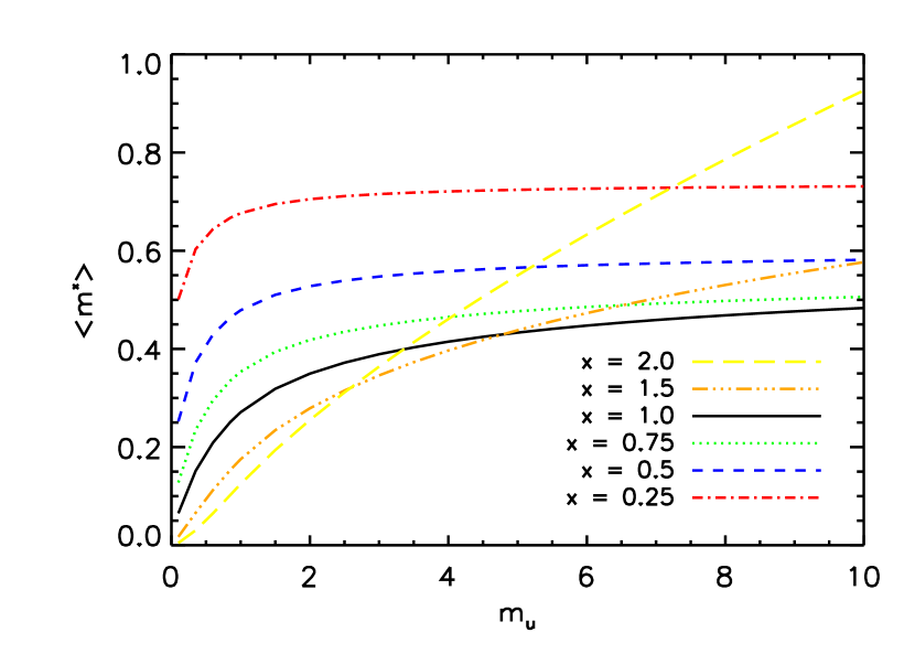
Figure 2.— Average values of powers of the protostellar mass, ${\langle m^{x}\rangle}$, weighted by the Chabrier (2005) IMF for different powers of $x$ as a function of the upper mass limit in the cluster, ${m_{u}}$.

4. Results for the Steady-State PMF

4.1. Analytic Results for a Salpeter IMF

In order to see how the different accretion histories affect the PMF, we first consider a Salpeter IMF (Salpeter, 1955),

$$\psi_{\rm Sal}({m_{f}})\simeq 1.35\left(\frac{{m_{\ell}}}{{m_{f}}}\right)^{1.35}~{}~{}~{}~{}({m_{\ell}}\leq{m_{f}}\leq{m_{u}}),$$ (42)

where we have neglected the factor $({m_{\ell}}/{m_{u}})^{1.35}$ compared to unity in the normalization. For the case in which ${m_{u}}$ is very large, the average mass ${\langle{m_{f}}\rangle}=(1.35/0.35){m_{\ell}}$; thus, to get an average mass of $0.5M_{\odot}$, for example, requires ${m_{\ell}}=0.13M_{\odot}$. To compare with results from the truncated Chabrier IMF below, we also consider the case in which ${m_{u}}=3M_{\odot}$ and ${\langle{m_{f}}\rangle}=0.4M_{\odot}$; this requires ${m_{\ell}}=0.16M_{\odot}$.

Since we are looking for simple analytic results in this subsection, we focus on the case of untapered accretion. The average star-formation time is then (eq. 25)

$${\langle t_{f}\rangle}=\frac{1.35{m_{\ell}}^{1-{j_{f}}}\phi({j_{f}})}{0.35+{j_{f}}}\;t_{f1},$$ (43)

where

$$\phi({j_{f}})=\left[1-\left(\frac{{m_{\ell}}}{{m_{u}}}\right)^{0.35+{j_{f}}}\right].$$ (44)

For Isothermal Sphere accretion, ${\langle t_{f}\rangle}$ is just ${\langle{m_{f}}\rangle}t_{f1}$, or about half the time to form a one solar mass star if the mean mass is about $0.5M_{\odot}$.

With the aid of equation (23), the PMF in equation (14) becomes

$$\psi_{p}(m) = \frac{m}{{\langle t_{f}\rangle}}\int_{m_{f,\ell}}^{m_{u}}\frac{\psi_{\rm Sal}({m_{f}})}{\dot{m}}\;d\ln{m_{f}},$$ (45)

$$= \frac{1.35{m_{\ell}}^{1.35}m^{1-j}}{\dot{m}_{1}{\langle t_{f}\rangle}}\int_{m_{f,\ell}}^{m_{u}}\frac{d\ln{m_{f}}}{{m_{f}}^{\alpha}},$$ (46)

$$= \frac{(1-j)(0.35+{j_{f}}){m_{\ell}}^{0.35+{j_{f}}}m^{1-j}}{\alpha\phi({j_{f}}){m_{f,\ell}}^{\alpha}}\;f({m_{f,\ell}}),~{}~{}~{}~{}~{}$$ (47)

where

$$\alpha\equiv 1.35+{j_{f}}-j$$ (48)

and

$$f(m)\equiv 1-\left(\frac{m}{{m_{u}}}\right)^{\alpha}.$$ (49)

For masses large enough to be included in the IMF ($m>{m_{\ell}}$), we have ${m_{f,\ell}}=m$, so that

$$\psi_{p}(m)\propto m^{-(0.35+{j_{f}})}f(m).$$ (50)

There are several points to note about this result for the PMF. First, since it is weighted by the accretion time, it is much flatter in the mass range ${m_{\ell}}\leq m\ll{m_{u}}$ for Isothermal Sphere accretion ($\psi\propto m^{-0.35}$) than for Turbulent Core accretion ($\psi\propto m^{-1.1}$) or Competitive Accretion ($\psi\propto m^{-1.35}$); indeed, since all stars have the same formation time in the latter model, it just mimics the original Salpeter IMF. The Turbulent Core and Competitive Accretion models are shifted to lower masses compared to the Isothermal Sphere accretion model since they have longer accretion times at low mass, as shown in equation (28).

Second, the PMF becomes depleted as $m\rightarrow{m_{u}}$, since $f(m)\rightarrow 0$ there. This occurs because protostars with final masses close to ${m_{u}}$ spend most of their lives at lower masses as they grow by accretion; only a small number of protostars are actually in the final stages of growth.

Third, the PMF is independent of the overall rate of star formation. This was clear from our general expression for the PMF (eq. 14), in which $\psi_{p}\propto t_{\rm acc}/{\langle t_{f}\rangle}$ depends on the ratio of two star-formation times.

The final point to note is that the coefficient in $\psi_{p}(m)$ can be small, particularly as $j\rightarrow 1$; thus, most of the protostars can be at low masses. Evaluation of the mean protostellar mass using equation (41) shows that it is much less for the Turbulent Core and Competitive Accretion models than for the Isothermal Sphere model. For example, consider the case in which ${m_{\ell}}=0.16M_{\odot}$ and ${m_{u}}=3M_{\odot}$; we find that the average protostellar mass is $(0.38,\,0.16,\,0.10)\,M_{\odot}$ for Isothermal Sphere accretion, the Turbulent Core model and Competitive Accretion, respectively.

4.2. Results for the Chabrier IMF

The Salpeter IMF has the benefit of being easily integrable, but it is inaccurate at low masses. In this section we derive the mean mass for each accretion model using the Chabrier (2005) IMF:

$$\psi_{C} = \psi_{1}\exp-\left[\frac{(\log m-\log 0.2)^{2}}{2\times 0.55^{2}}\right]$$ (51)

$$~{}~{}~{}~{}~{}~{}~{}~{}~{}~{}~{}~{}~{}~{}~{}~{}~{}(m_{l}\leq m\leq 1M_{\odot}),$$

$$\psi_{C} = \psi_{2}m^{-1.35}~{}~{}~{}~{}~{}(m\geq 1M_{\odot}).$$ (52)

The Chabrier IMF is log-normal below 1 $M_{\odot}$ and Salpeter above. The constants are determined by continuity and by enforcing: $\int_{m_{l}}^{m_{u}}\psi(m)\;d\;\mbox{ln}\ m=1$. In this section, we adopt fiducial values of $m_{\ell}\sim 0.033~{}M_{\odot}$ and $m_{u}=3.0~{}M_{\odot}$, which yield $\psi_{1}\simeq 0.35$ and $\psi_{2}\simeq 0.16=\psi_{C}(1)$. With these coefficients, $\psi_{C}$ gives an average stellar mass (including brown dwarfs) of ${\langle m_{*}\rangle}\simeq 0.4~{}M_{\odot}$

The PMF derived in equation (7) can be expressed in terms of the Chabrier IMF, $j$, $j_{f}$, and $m_{u}$. The Two-Component Turbulent Core model also depends upon the ratio ${\cal R}_{\dot{m}}=\dot{m}_{\rm TC}/\dot{m}_{\rm S}$. For the numerical examples presented in this paper, we set the star-formation times for the Isothermal Sphere and Turbulent Core models to be equal, which the data in Table 2 show corresponds to ${\cal R}_{\dot{m}}=3.6$. ${\cal R}_{\dot{m}}$ exceeds unity because it is evaluated for $1M_{\odot}$ stars; for this value of ${\cal R}_{\dot{m}}$, the ratio of the accretion rates tor the two models is close to unity for protostars of typical mass. Estimates of the star-formation time have typically been based on the Class 0 lifetime, where most of the mass accretion was assumed to take place. However, observations by Enoch et al. (2008) indicate that the protostellar luminosities in the Class 0 and Class I phases are not substantially different, suggesting that significant accretion continues through much of the Class I phase. For untapered accretion, the PMF (eq. 7) for the IS, TC and CA models is

$$\psi_{p}(m)=(1-j)m^{1-j}\frac{\int_{m_{f,\ell}}^{m_{u}}\psi_{C}({m_{f}}){m_{f}}^{j-j_{f}}\;d\ln{m_{f}}}{\int_{m_{\ell}}^{m_{u}}\psi_{C}({m_{f}}){m_{f}}^{1-{j_{f}}}\;d\ln{m_{f}}},$$ (53)

where we used equations (23) and (25) to evaluate the the acceleration time ($t_{\rm acc}\propto 1/\dot{m}$) and the mean formation time that enter the PMF. For tapered accretion, a factor $[1-(m/{m_{f}})^{1-j}]^{1/2}$ must be included in the integrand in the numerator (see eq. 35). We plot the PMF for the four models in Figure 3 assuming that $m_{u}=3M_{\odot}$. The Isothermal Sphere PMF peaks significantly to the right of the other models. As a result, it predicts a higher fraction of relatively massive protostars in the distribution than any of the other models, including the Chabrier IMF. This is a direct consequence of the weighting by the star-formation time, in which more massive stars have the longest accretion times in the Isothermal Sphere case. The Competitive Accretion and Turbulent Core PMFs contain fewer massive protostars than the Isothermal Sphere PMF because protostars in those models accrete more rapidly as they approach their final mass, thereby reducing the time they spend in the PMF.

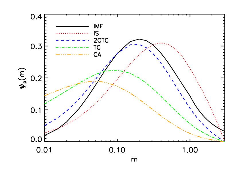
Figure 3.— The PMF for the four models with untapered accretion where $m_{u}=3~{}M_{\odot}$. The Chabrier IMF is given by the solid line. For the Two-Component Turbulent Core model, we adopt ${\cal R}_{\dot{m}}=3.6$.

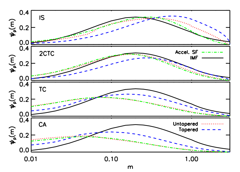
Figure 4.— The PMF for the four models with untapered accretion(dotted), tapered accretion (dashed), and untapered accretion with accelerating star formation (dot-dashed), where $m_{u}=3~{}M_{\odot}$. The Chabrier IMF is given by the solid line. For the Two-Component Turbulent Core model, we adopt ${\cal R}_{\dot{m}}=3.6$. For the accelerating star formation models we use $\tau=1$ Myr.

The mean protostellar mass, ${\langle m\rangle}_{p}$, is given by equation (41). With the Chabrier IMF, the Isothermal Sphere, Turbulent Core, and Competitive Accretion models give ${\langle m\rangle}_{p}=0.47,0.16,0.09M_{\odot}$, respectively, assuming that $m_{u}=3~{}M_{\odot}$. The Isothermal Sphere mean value is larger than that derived in the previous section using the Salpeter IMF with $m_{l}=0.16M_{\odot}$ since the Chabrier IMF turns over at $0.2M_{\odot}$, so that the lower masses contribute less weight to the mean than in the case of the Salpeter IMF. The ordering of the values of the mean mass for these three models follows from the ordering of the values of the accretion time (eq. 28), since $t_{\rm acc}$ is the weighting factor that enters the PMF (eq. 14) and it is largest at small masses for the Competitive Accretion model and smallest for such masses for the Isothermal Sphere model.

Figure 5 shows ${\langle m\rangle}_{p}$ as a function of the maximum cluster mass. The Isothermal Sphere model has a significantly higher mean protostellar mass than the stellar IMF as a result of the long formation times of more massive stars. In the Competitive Accretion and Turbulent Core models, the accretion rate accelerates with time so that protostars spend a larger fraction of their lifetime at low masses than in the Isothermal Sphere case, in which the accretion rate is independent of mass. Note that we assume that the Isothermal Sphere model is suitable only for stars below $5~{}M_{\odot}$. When the accretion rate is modulated by turbulence, as in the Two-Component Turbulent Core model, the mean mass rises less steeply than for a pure isothermal sphere as a function of cluster mass upper limit.

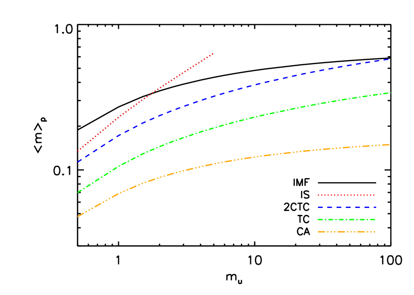
Figure 5.— The mean mass (eq. 41) of the PMF, ${\langle m\rangle}_{p}$, for the four models as a function of $m_{u}$ in the untapered, non-accelerating case. The Chabrier IMF mean is shown by the solid line. For the Two-Component Turbulent Core model we adopt ${\cal R}_{\dot{m}}=3.6$. We restrict the Isothermal Sphere curve to ${m_{u}}\leq 5~{}M_{\odot}$.

Figure 6 shows the ratio of the median to the mean protostellar mass as a function of the maximum stellar mass in the cluster, $m_{u}$, for each of the accretion models. This ratio decreases with $m_{u}$ since the mean mass increases with $m_{u}$ whereas the median mass is relatively insensitive to it. Since larger clusters can sample the rarer, more massive stars in the IMF, we expect large clusters to have small ratios of the median to mean protostellar masses, particularly for the Competitive Accretion and Turbulent Core models. Furthermore, since the accretion luminosity is proportional to the mass and the accretion rate, this graph suggests that the Protostellar Luminosity Functions will be quite different for the different models, although we expect the differences to be less for tapered accretion (Paper II).

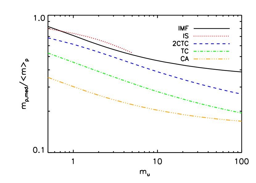
Figure 6.— The ratio of the median to mean protostellar mass of the PMF for the four models as a function of $m_{u}$ with non-accelerating untapered accretion. We adopt ${\cal R}_{\dot{m}}=3.6$ model. The value for the Chabrier IMF is indicated by the solid line. Since the Isothermal Sphere model is primarily for low-mass stars, we restrict it to ${m_{u}}\leq 5~{}M_{\odot}$.

The maximum expected protostellar mass, ${m_{p,\,\rm max}}$, in a cluster of ${\cal N}_{p}$ protostars is given by

$$\frac{1}{{\cal N}_{p}}=\int_{{m_{p,\,\rm max}}}^{m_{u}}d\ln{m_{f}}\psi_{p}({m_{f}})\,\\$$ (54)

The resulting values of ${m_{p,\,\rm max}}$ are portrayed in Figure 7. The plot illustrates that the expected value of the maximum protostellar mass, ${m_{p,\,\rm max}}$, for the Competitive Accretion and Turbulent Core models with ${\cal N}_{p}\lower 2.15277pt\hbox{$\;\buildrel<\over{\sim}\;$}100$ stars can be significantly less than the maximum stellar mass, ${m_{u}}$, which is determined by the Class II stars in the cluster that obey a normal IMF.

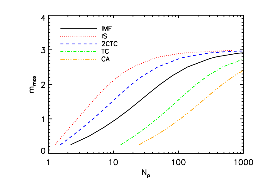
Figure 7.— The maximum protostellar mass, ${m_{p,\,\rm max}}$ as a function of the number of protostars, ${\cal N}_{p}$ in the untapered, non-accelerating case. The maximum stellar mass is $m_{u}=3~{}M_{\odot}$. We adopt ${\cal R}_{\dot{m}}=3.6$ for the Two-Component Turbulent Core model.

5. Accelerating Star Formation

From an analysis of the pre-main-sequence stars in the Orion Nebula Cluster, Palla & Stahler (1999) concluded that the star formation there has been accelerating. Palla & Stahler (2000) extended this analysis to seven other star-forming regions and found evidence for acceleration in all but one case. They attributed this acceleration to contraction of the parent molecular cloud, which they surmised was a quasi-static process. They inferred exponentiation times ranging from 1.0 Myr for $\rho$ Oph and IC 348 to 3.3 Myr for NGC 2264. The shortest of these acceleration times is not that much greater than the typical star-formation time of 0.54 Myr found by Evans et al. (2009). Here we determine the effect of accelerated star formation on the PMF.

The evolution of the PMF in time is governed by a continuity equation. To conform with standard practice, we define $n(m,{m_{f}},t)dmd{m_{f}}$ as the number of protostars in the mass range $dm$ and final mass range $d{m_{f}}$ at time $t$. Under the assumption that the stars are born with an initial mass function $\psi({m_{f}})$, the continuity equation for $n$ is then

$${{\partial n}\over{\partial t}}+{{\partial\hfil}\over{\partial m}}(n\dot{m})=\dot{\cal N}_{*}(t)\delta(m)\;\frac{\psi({m_{f}})}{{m_{f}}},$$ (55)

where $\dot{\cal N}_{*}(t)$ is the rate at which stars are born at time $t$, $\delta(x)$ is the delta function, and the factor ${m_{f}}^{-1}$ allows from the conversion from $n\,d{m_{f}}$ to $\psi\,d\ln{m_{f}}$. The Green’s function for this problem, which we denote by $G(t-t_{0})$, is the solution for $\dot{\cal N}_{*}(t)=\delta(t-t_{0})$. Writing the protostellar mass as an explicit function of time, $m=\mu(t-t_{0})$, we have

$$G(t-t_{0})=\delta[m-\mu(t-t_{0})]\,\frac{\psi({m_{f}})}{{m_{f}}}\,H(t-t_{0}),$$ (56)

where $H(t-t_{0})$ is the Heaviside step function. The general solution is then

$$n = \int_{-\infty}^{\infty}G(t-t_{0})\dot{\cal N}_{*,0}dt_{0},$$ (57)

$$= \int_{-\infty}^{t}\delta[m-\mu(t-t_{0})]\,\frac{\psi({m_{f}})}{{m_{f}}}\,\dot{\cal N}_{*,0}dt_{0}.~{}~{}~{}~{}$$ (58)

Note that $t-t_{0}$ is the age of a star at time $t$ that was born at time $t_{0}$. Let $t_{m}$ be the age of a star of mass $m$ and final mass ${m_{f}}$. We can then rewrite the $\delta$-function as

$$\delta[m-\mu(t-t_{0})]=\frac{\delta(t-t_{0}-t_{m})}{\dot{m}},$$ (59)

where $\dot{m}=d\mu/dt$ is the accretion rate. The solution is then

$$n(m,{m_{f}},t)=\frac{\psi({m_{f}})\dot{\cal N}_{*}(t-t_{m})}{{m_{f}}\dot{m}}.$$ (60)

To convert this to the bivariate PMF, note that

$$\psi_{p2}(m,{m_{f}},t)=\frac{n(m,{m_{f}},t)\,m{m_{f}}}{\int_{m_{\ell}}^{m_{u}}d{m_{f}}\int_{0}^{m_{f}}dm\,n(m,{m_{f}},t)},$$ (61)

so that

$$\psi_{p2}=\frac{\psi({m_{f}})\displaystyle\frac{m}{\dot{m}}\,\dot{\cal N}_{*}(t-t_{m})}{\int_{m_{\ell}}^{m_{u}}d\ln{m_{f}}\psi({m_{f}})\int_{0}^{t_{f}}dt_{m}\,\dot{\cal N}_{*}(t-t_{m})}.$$ (62)

In a steady state [$\dot{\cal N}_{*}(t-t_{m})=$ const], this reduces to the result given in equation (13). The protostellar mass function for an arbitrary star formation history is then obtained by inserting this result into equation (7).

As a simple model of accelerating star formation, we assume an exponentially increasing birthrate,

$$\dot{\cal N}_{*}(t-t_{m})=\dot{\cal N}_{*,0}e^{(t-t_{m})/\tau},$$ (63)

where $\dot{\cal N}_{*,0}=\dot{\cal N}_{*}(t=0)$ is the current birthrate. Substituting into equation (62), we find

$$\psi_{p2}=\frac{\psi({m_{f}})t_{\rm acc}\exp-(t_{m}/\tau)}{\tau{\langle 1-\exp(-t_{f}/\tau)\rangle}}.$$ (64)

The PMF is then

$$\psi_{p}(m) = \frac{1}{\tau{\langle 1-\exp(-t_{f}/\tau)\rangle}}\times$$ (65)

$$\int_{m_{f,\ell}}^{m_{u}}\psi({m_{f}})t_{\rm acc}e^{-t_{m}/\tau}d\ln{m_{f}},$$

which reduces to equation (7) for $\tau\rightarrow\infty$.

The PMF depends on the time scale $t_{m}$, the age of a protostar of mass $m$ and final mass ${m_{f}}$. If the accretion is untapered, then the protostellar mass grows according to equation (24) and $t_{m}$ is given by

$$t_{m}=t_{f1}\,\frac{m^{1-j}}{{m_{f}}^{{j_{f}}-j}}.$$ (66)

For the Two-Component Turbulent Core model, $t_{m}$ is given by

$$t_{m}={{2}\over{\dot{m}_{S}}}{\sqrt{{\cal R}_{\dot{m}}^{2}{m_{f}}^{1/2}m+1}-1\over{{\cal R}_{\dot{m}}^{2}{m_{f}}^{1/2}}}.$$ (67)

The value of $t_{m}$ for the case of tapered accretion has been given in equation (33). Figure 4 shows $\psi_{p}(m)$ in the accelerating case with untapered accretion. We consider the case with $\tau=1$ Myr, which is approximately twice the average star-formation time. In comparison to the steady star formation (dotted lines), the PMF peaks are shifted towards lower masses for accelerating star formation except in the Competitive Accretion case, where the peak mass increases from $\sim 0.05M_{\odot}$ to $\sim 0.08M_{\odot}$.

6. Comparison with Observations

6.1. The Star Formation Timescale

As discussed in the Introduction, it is not presently possible to directly measure the masses of the protostars in a star-forming region. The protostellar luminosity function is subject to direct observation and will be discussed in Paper II. Nonetheless, it is possible to carry out an approximate comparison between observation and theory by comparing the average star-formation time observed in low-mass star-forming regions with the theoretical values predicted in §3.

First, we show that the average observed star-formation time as determined by number counts is the IMF-averaged formation time, ${\langle t_{f}\rangle}$, not the PMF-averaged formation time, ${\langle t_{f}\rangle}_{p}$. Evans et al. (2009) determined the average star-formation time, ${\langle t_{f}\rangle}_{\rm obs}$, by comparing the number of protostars with the number of Class II sources:

$$\frac{{\langle t_{f}\rangle}_{\rm obs}}{{\langle t_{\rm II}\rangle}}=\frac{{\cal N}_{p}}{{\cal N}_{\rm II}},$$ (68)

where ${\cal N}_{\rm II}$ and ${\langle t_{\rm II}\rangle}$ are the number and average lifetime of Class II sources. Although nothing is known at present about the mass dependence of the Class II lifetime, we allow for the possibility that there is such a dependence by using the IMF-averaged value, ${\langle t_{\rm II}\rangle}$, in this equation. The number of protostars is just the star-formation rate times the IMF-averaged lifetime (eq. 10), and similarly, the number of Class II sources is just ${\cal N}_{\rm II}=\dot{\cal N}_{*}{\langle t_{\rm II}\rangle}$. As a result, we have

$$\frac{{\langle t_{f}\rangle}_{\rm obs}}{{\langle t_{\rm II}\rangle}}=\frac{\dot{\cal N}_{*}{\langle t_{f}\rangle}}{\dot{\cal N}_{*}{\langle t_{\rm II}\rangle}}=\frac{{\langle t_{f}\rangle}}{{\langle t_{\rm II}\rangle}},$$ (69)

so that

$${\langle t_{f}\rangle}_{\rm obs}={\langle t_{f}\rangle}.$$ (70)

Thus, the mean formation time inferred from the ratio of the number of protostars to the number of Class II sources is equal to the IMF-averaged value of the formation time. By contrast, if there were a method of determining the formation time of each observed protostar, the average of these times, ${\langle t_{f}\rangle}_{p}=\int d\ln m\psi_{p}(m)t_{f}$, would be quite different. We generalize this expression to the case of accelerating star formation in the Appendix.

Table 3Star-Forming Region Properties

Region	$T$ (K)	$\Sigma$ (g cm-2)	$\bar{n}_{\rm H}$ ($10^{4}$ cm${}^{-3})$	${\langle t_{\rm 0,I}\rangle}$ (Myr)
Perseus	10-13	0.06	1.0	0.72
Serpens	10-15	0.06	0.9	0.56
Ophiuchus	12-20	0.08	1.4	0.40
Average		0.07	1.1	0.56

Evans et al. (2009) report an average star-formation time, ${\langle t_{f}\rangle}$, of 0.54 Myr after correcting for extinction for five local star-forming regions. This value is the sum of the estimated Class 0 and Class I lifetimes and assumes a Class II lifetime of 2 Myr. Evans et al. (2009) find that the lifetimes vary significantly over their sample of clouds, where the lowest lifetimes correspond to the smallest clouds containing the fewest protostars. The lifetimes have an uncertainty of order $\pm$ 0.1 Myr. In our comparison, we focus on Perseus, Ophiuchus, and Serpens, which are much more massive than Lupus and Cha II. They have a combined average star-formation time of 0.56 Myr.

As discussed in the Introduction, by adopting the protostellar lifetimes from Evans et al. (2009), we implicitly assume a direct mapping between Class 0, I and Stage 0, I. The core mass estimates obtained for these regions by Enoch et al. (2009) support this assumption for both Perseus and Serpens since all but one Class I envelope exceed $0.1M_{\odot}$ in Perseus and none in Serpens. In contrast, Enoch et al. (2009) report that about half of the $\rho$ Ophiuchus Class I sources have envelopes with masses $<0.1M_{\odot}$, so that they are not true protostars by our definition. This suggests that the value of ${\langle t_{f}\rangle}_{\rm obs}$ we adopt from Evans et al. (2009), which includes the Class I sources with envelopes less than $0.1M_{\odot}$, overestimates the mean protostellar lifetime in that region. Since Ophiuchus already has the shortest lifetime of the three clusters we consider, it is possible that the rate of star formation in this cluster has recently slowed down. Bearing in mind these caveats, in our comparison we adopt conservative error estimates that are comparable to the error resulting from the inclusion of the small-envelope sources.

To compare with the observations, we use the more evolved Class II sources to estimate the cluster upper mass limit, $m_{u}$. Since the Class II sources are about three times more numerous than the Class 0 and Class I objects, their luminosities provide a reasonable expectation for the most massive star forming in the cluster. Evans et al. (2009) report a maximum extinction corrected Class II luminosity of $\sim 90L_{\odot}$, suggesting a maximum stellar mass of $\sim 3M_{\odot}$ (Palla & Stahler, 1999). As a counterpoint, if we assume that the combined population of Class II sources is drawn from the Chabrier IMF with maximum stellar mass of 120 $M_{\odot}$ then a statistical argument suggests that 12 of the Class II objects should have masses greater than $3~{}M_{\odot}$. Perseus, containing 244 Class II sources, should have five such stars. This difference between the observed IMF and the expected one is partially due to selection, since the clusters were chosen to have only low-mass stars. It is also possible that the conditions in these clouds work against the formation of massive stars.

We use the model definitions from Table 2 to infer the physical parameters for each model given an average star-formation time of ${\langle t_{f}\rangle}=0.56$ Myr. We give the observed physical parameters values for local molecular clouds in Table 3. Each of the models constrains a different physical parameter (Table 4). For the Competitive Accretion model, the relevant star-formation time, ${\langle t_{f}\rangle}$, is about equal to the freefall time of the entire clump, so that the lifetime depends only upon the average density. For the Two-Component Turbulent Core model, we assume that the thermal and turbulent contributions to the accretion are comparable by setting ${\cal R}_{\dot{m}}=3.6$ (see §4.2). (The Turbulent Core model was developed for high-mass star formation, and the Turbulent Core contribution grows in importance as the stellar mass increases, eq. 19.)

To compare the models with accelerating star formation with observation, we first use a least-squares approach to re-analyze the data assembled by Palla & Stahler (2000), who fit their data “by eye.” We find $\tau=0.9$ Myr for Ophiuchus, in good agreement with the Palla & Stahler (2000) value of $\tau=1$ Myr. At face value, this suggests that star formation is rapidly accelerating. However, the ages of stars included in the fit are greater than 0.5 Myr, so that one cannot use this trend to reliably infer information about more recent star formation activity. To emphasize this point, observations by Enoch et al. (2009) find only 3 Class 0 sources, which, when compared to the relatively larger numbers of Class I sources, suggest that current star formation in Ophiuchus is likely decelerating. A fit of IC348, an active region of Perseus, gives $\tau=2.2$ Myr rather than 1 Myr as reported by Palla & Stahler (2000). Several other regions discussed by Palla & Stahler (2000) show a turnover in the number of stars at recent times, further highlighting the point that the star formation rate may not be monotonic and is not necessarily well represented by a single exponential. Despite this caveat, we select $\tau=2$ Myr as a fiducial value. For Perseus and Ophiuchus, we individually adopt $\tau=2$ Myr and $\tau=1$ Myr, respectively. We adopt 2 Myr for the Class II lifetime, which is the same value Evans et al. (2009) use to estimate the observed protostellar lifetime. Note that it is possible that the Class II lifetime depends on stellar mass, but in the absence of any relevant data we neglect this possibility here.

The results summarized in Tables 3-5 show the inferred physical conditions in an average star-forming cloud (like Serpens), in Perseus and in Ophiuchus for each model for the cases of tapered and untapered accretion, accelerating and non-accelerating star formation. The inferred temperatures for the Isothermal Sphere and Two-Component Turbulent Core models are closer to the observed values when tapering and/or acceleration is allowed for. Tapering or allowing for acceleration gives a good fit for both the Turbulent Core model and the Competitive Accretion model in Perseus. In Serpens, non-accelerating star formation with untapered or tapered accretion gives good agreement for these models. In Ophiuchus, both models do best for the untapered, non-accelerating case.

However, as discussed in §3 above, the accretion rates for the various models are uncertain for several reaons: they do not allow for the effects of protostellar winds in disrupting the protostellar cores, they do not allow for an initial infall velocity, and they do not include the effects of magnetic fields. As a result of these competing effects, the fiducial accretion rate coefficients in Table 2 may be either higher or lower than those we have adopted, thus impacting our estimates of the physical parameters. If we assume that this uncertainty is a factor two in the accretion rate, then this corresponds to a factor $2^{2/3}\simeq 1.6$ in the inferred temperature in the Isothermal Sphere model, a factor $2^{4/3}\simeq 2.5$ in the inferred column density in the Turbulent Core model, and a factor $2^{2}=4$ in the inferred density in the Competitive Accretion model. It must also be borne in mind that there are uncertainties in the observed values of the physical parameters describing the clouds, particularly the lifetimes. With allowance for an overall factor of two uncertainty in the accretion rate relative to the actual values, we summarize the consistency between the models and observed regions in Table 7. We find that the Isothermal Sphere model is consistent with the data for both Perseus and Ophiuchus for all but the non-accelerating, untapered model. One might question this consistency, given that the temperature is known to much better than the factor 1.6 we are allowing; however, we are allowing for uncertainty in the coefficient of $T^{3/2}$ in equation (15), not for errors in the temperature. The Two-Component Turbulent Core model is consistent with the data for all but the non-accelerating, untapered model; it would have the same level of consistency with the data as the IS model if ${\cal R}_{{\dot{m}}}$ were lowered from 3.6 to 1.7. (Based on eq. 27, this corresponds to increasing the value of ${m_{f}}$ for which $t_{f}$ is closer to the TC case than to the IS case from about $0.5\,M_{\odot}$ to about $1.2\,M_{\odot}$.) The Turbulent Core and Competitive Accretion models are consistent with the Perseus data for all but the non-accelerating, tapered model, but they are consistent with the Serpens and Ophiuchus data only for the non-accelerating models.

We note that the free-fall time corresponding to the mean density in the regions we have considered is $t_{\rm ff}\simeq 0.4$ Myr, which is comparable to the mean star formation times (which is consistent with Competitive Accretion), but short compared to the acceleration time. Conceptually, the Competitive Accretion model involves rapid acceleration, but numerical simulations are needed to determine whether the observed relatively long acceleration times are consistent with the model.

Since a number of the models predict reasonable physical parameters, uncertainty in the mean temperatures, densities, columns, and lifetimes contributes to our inability to determine which models are consistent with observation. For comparison in the context of these uncertainties, we plot the physical parameters of each of the model as a function of ${\langle t_{\rm obs}\rangle}$ in Figure 8. This plot also illustrates that in all cases the inferred temperature, column density, and density increase with decreasing star-formation times.

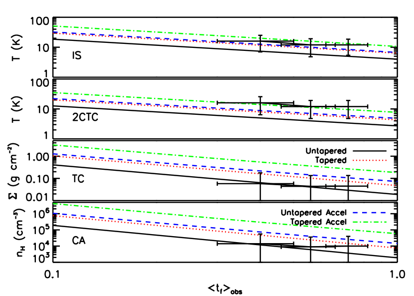
Figure 8.— The physical parameter for each model versus the observed star-formation time, ${\langle t_{f}\rangle}_{\rm obs}$. We assume $n=1$, $\tau=1$ Myr, and ${\langle t_{\rm II}\rangle}=2$ Myr in the tapered and accelerating cases. Ophiuchus (left), Serpens (middle), and Perseus (right) are overlaid with horizontal error bars for the uncertainty in the measurements and vertical error bars for the uncertainty due to the model accretion rates.

6.2. Discussion

In this section, we address various sources of uncertainty inherent in the calculations. As described in §3.1, the instantaneous accretion rate may be larger than estimated at early times and may fluctuate strongly on short timescales. We have also neglected possible temporal variations in the core star formation efficiency–i.e., the fraction of the mass in the core that actually accretes onto the star–in modeling the protostellar accretion rate. Finally, the values of $n$, ${\langle t_{\rm II}\rangle}$ and $\tau$ have some intrinsic uncertainty and may vary between clouds. We discuss these three parameters below.

Tapering of the accretion is very plausible, since we expect accretion to decrease as the infall phase ends and the core mass is depleted. Measurements of the protostellar luminosity appear inconsistent with constant or increasing accretion through the Class I phase, a topic we shall address in Paper II. However, there are no direct estimates of $n$, and the exact tapering function is poorly constrained by observation. Unfortunately, we find that we cannot definitively constrain $n$ on the basis of the observed star-formation time due to variation between clouds and uncertainties in both the physical parameters and the accretion models, as discussed above.

Evans et al. (2009) estimate an uncertainty of $\pm 1$ Myr for the Class II lifetime, a variation of 50%. As shown by equation (68), the observed star-formation time varies directly as ${\langle t_{\rm II}\rangle}$ in the non-accelerating case. The accretion rate then varies as $1/{\langle t_{\rm II}\rangle}$, so that $T^{3/2}\propto 1/{\langle t_{\rm II}\rangle}$ in the Isothermal Sphere case, $\Sigma^{3/4}\propto 1/{\langle t_{\rm II}\rangle}$ in the Turbulent Core case, and $n_{\rm H}^{1/2}\propto 1/{\langle t_{\rm II}\rangle}$ in the Competitive Accretion case. Thus, a longer Class II lifetime would decrease the inferred temperature, column density and density accordingly. Our analysis in §6.1 suggests that a longer Class II phase would worsen agreement of the Isothermal Sphere and Two-Component Turbulent Core models with the observations, since the implied temperatures are already somewhat low in most cases. Conversely, a shorter Class II lifetime would improve agreement with observation for many of these models, with the exception of the tapered, accelerating Isothermal Sphere model for Ophiuchus.

As discussed in §5, Palla & Stahler (2000) derived $\tau$ values between $\sim 1-3$ Myr for a collection of eight clouds. They performed the fits by eye so that their estimates of the e-folding time are not precise. We used a least-squares fit to get improved values for the acceleration times, but it must be borne in mind that the actual star formation histories may be much more complex than the simple exponential form that we have used to fit them.

Table 4Model Properties for ${\langle t_{f}\rangle}_{\rm obs}=0.56$ Myr

		Non-Accelerating		Accelerating
Model	Parameter	Untapered	Tapered	Untapered	Tapered
Isothermal Sphere	$T$(K)	5.9	9.3	7.8	12
2C Turbulent Core	$T$(K)	3.9	6.1	5.4	8.6
Turbulent Core (TC)	$\Sigma$ (g cm-2)	0.041	0.10	0.083	0.21
Competitive Accretion	$\bar{n}_{\rm H}$ ($10^{4}$ cm-3)	0.60	2.4	1.8	7.1

Table 5Model Properties for ${\langle t_{f}\rangle}_{\rm obs}=0.72$ Myr: Perseus

			Non-Accelerating		Accelerating
Model	Parameter	Observed Value	Untapered	Tapered	Untapered	Tapered
Isothermal Sphere	$T$ (K)	10-13	5.0	7.9	6.6	10
2C Turbulent Core	$T$ (K)	10-13	3.3	5.2	4.6	7.3
Turbulent Core (TC)	$\Sigma$ (g cm-2)	0.06	0.029	0.074	0.061	0.15
Competitive Accretion	$\bar{n}_{\rm H}$ ($10^{4}$ cm-3)	1.0	0.37	1.5	1.1	4.5

Table 6Model Properties for ${\langle t_{f}\rangle}_{\rm obs}=0.40$ Myr: Ophiuchus

			Non-Accelerating		Accelerating
Model	Parameter	Observed Value	Untapered	Tapered	Untapered	Tapered
Isothermal Sphere	$T$ (K)	12-20	7.4	12	13	20
2C Turbulent Core	$T$ (K)	12-20	4.8	7.7	8.7	14

Turbulent Core (TC) & $\Sigma$ (g cm^-2) 0.08 0.064 0.16 0.22 0.55
Competitive Accretion $n_{\rm H}$ ($10^{4}$ cm^-3) 1.4 1.2 4.7 7.4 30

Table 7Model Summary

	Ophiuchus				Serpens				Perseus
Model	UN	TN	UA	TA	UN	TN	UA	TA	UN	TN	UA	TA
Isothermal Sphere	✓	✓	✓	✓	✓	✓	✓	✓	o	✓	✓	✓
2C Turbulent Core	o	✓	✓	✓	o	✓	✓	✓	o	✓	✓	✓
Turbulent Core (TC)	✓	✓	o	o	✓	✓	o	o	✓	✓	✓	o
Competitive Accretion	✓	✓	o	o	✓	✓	o	o	✓	✓	✓	o

7. CONCLUSIONS

We have analyzed the Protostellar Mass Function (PMF), which is the Present-Day Mass Function (PDMF) of a cluster of protostars. The PMF builds on the IMF, which measures the final mass distribution of a cluster of stars after completion of the formation process. The PMF depends on the mass dependence of the formation time of the stars, $t_{f}$, and therefore can in principle provide an observational diagnostic of theories of star formation. Direct observation of the PMF must await further observational and theoretical advances, since it is not currently possible to infer the mass for protostars because they are generally extremely obscured and the luminosity is dominated by accretion. Nonetheless, it is possible to compare theoretical models with measurements of the mean lifetime of protostars in different molecular clouds as we have done here. Furthermore, the PMF is the basis for the Protostellar Luminosity Function, which is directly accessible to observation (Paper II).

We have made two key assumptions in inferring the PMF. First, since no stars above 3 $M_{\odot}$ are seen in the low-mass clusters we have analyzed (Evans et al., 2009; Enoch et al., 2009), we have assumed that none of the smaller number of protostars in these clusters will grow to more than $3M_{\odot}$; we therefore imposed an upper cutoff of $3M_{\odot}$ on the IMF in our analysis. Given the number of Class II sources, which have very nearly reached their final masses, we note that 12 Class II sources with $m>3M_{\odot}$ would be expected in these clusters based on a Chabrier (2005) IMF. These clusters were selected on the basis of their proximity so as to allow a thorough study of the Class 0, I, and II sources, so it is unlikely that this anomalous IMF is due to a selection effect. The second key assumption we have made is that the accretion rate is a simple function of only the current protostellar mass, the final mass and the time. We thus do not allow for variations in the accretion rate due to a brief high-accretion Larson-Penston phase or to temporal fluctuations in the accretion rate (although insofar as such fluctuations are random and there is a statistically large sample of protostars, they should not significantly affect the PMF).

We consider four accretion rate histories: the classical Isothermal Sphere accretion (Shu, 1977), the Turbulent Core model (McKee & Tan, 2002, 2003), a blend of the two (Two-Component Turbulent Core, 2C Turbulent Core), and an analytic approximation for the Competitive Accretion model (Bonnell et al., 1997, 2001a). There are substantial uncertainties in the accretion rates for each model: In all cases, one must allow for the effect of protostellar outflows, which can reduce the accretion rate by a factor of a few (Matzner & McKee, 2000). For the first three, there is a countervailing correction needed to allow for an initial infall velocity. Our approximation for the Competitive Accretion model captures many of its essential features, but since the model itself is based primarily on numerical simulations, there is no fully analytic form for it. In comparing the models with observation, we assume that the star formation is steady or accelerating; since the Competitive Accretion model has been developed for the evolution of individual star clusters, the comparison with observation is valid for this model only if a number of clusters are sampled, either because a forming cluster is comprised of a number of sub-clusters or because data from different clusters are averaged together.

The mean protostellar mass (Fig. 5) and the ratio of the median mass to the mean mass (Fig. 6) depend sensitively on the accretion history. The Turbulent Core and Competitive Accretion Models have accretion rates that increase with mass and therefore with time ($\dot{m}\propto m^{j}$, with $j=\frac{1}{2},\,\frac{2}{3}$ for the two models respectively). As a result, protostars of a given final mass, ${m_{f}}$, spend a smaller fraction of their lives at high mass than in the Isothermal Sphere model. Furthermore, these two models have accretion rates that increase with ${m_{f}}$, so that it takes less time to form a high-mass star than in the Isothermal Sphere model. Both effects are stronger for the Competive Accretion model. As a result, the mean protostellar mass increases systematically from the Competitive Accretion model to the Turbulent Core model to the Two-Component Turbulent Core model to the Isothermal Sphere model. The ratio of the median to mean protostellar mass follows the same ordering, and the same effect shows up in the plots of the PMF in Figure 3.

A common feature of all the accretion models is that the accretion rate remains constant or (usually) increases until the time at which the protostar reaches its final mass, when it abruptly ceases. In reality, as pointed out by Myers et al. (1998), the accretion will turn off gradually. To allow for this, we have inserted a factor $[1-(t/t_{f})^{n}]$ into the accretion rates; we refer to this as tapered accretion. In practice, we focused on the case $n=1$, which gives an accretion time $t_{f}$ twice as long as would be expected in the absence of tapering. This has the effect of increasing the temperature, column density or density of the model needed to match a given observed formation time. For example, in the Isothermal Sphere model, the accretion rate is proportional to $T^{3/2}$, so the temperature needed to match the observations of a given formation time is $2^{2/3}$ times greater for a tapered model than for an untapered one. Not only is tapering physically plausible, it also generally results in models that are in better agreement with observation. As shown in Figure 4, tapering moves the peak of the PMF to higher masses since stars spend a larger fraction of their lives at high mass when the accretion slows down at the end of the accretion process.

The rate of star formation should accelerate in time in a contracting gas cloud, and Palla & Stahler (2000) found direct evidence for such acceleration in a number of nearby star-forming clusters. We generalized our analysis of the PMF to the case in which the star formation rate is time dependent in §5. For simplicity, we have assumed that the acceleration applied only to the rate at which stars formed, not to the accretion rates of individual stars. This is a reasonably good approximation for the cases we analyzed, which have star-formation times that are significantly smaller than the time scale for acceleration. Moreover, the approximation is even better for for the Isothermal Sphere model, since the accretion rate depends on the temperature and radiative losses maintain an approximately constant temperature. On the other hand, the time scale for acceleration is often comparable to or less than the mean lifetime of Class II sources, so the ratio of the number of protostars to the number of Class II sources is larger than in the non-accelerating case. As a result, as shown in the Appendix, the “observed” star-formation time, which is given by equation (68), exceeds the actual star-formation time. We find that acceleration does not have a substantial effect on the PMF. Rather, its primary effect is to reduce the inferred time scale for the formation of individual stars, thereby increasing the inferred temperature, column density or mean density, depending on the accretion model.

In the absence of any direct information on protostellar masses, we were able to carry out only a very crude comparison with observation: Using the observed star-formation time scales in two different clusters, we computed the implied temperature (Isothermal Sphere model), surface density (Turbulent Core model), and mean density (Competitive Accretion model), and then compared with the observed values of these parameters. We found that the tapered accretion and accelerating star formation models were somewhat better than untapered, non-acceleration models, but we could not draw any firm conclusions due to uncertainties in both the observations and in the models, which have accretion rates that are probably uncertain by a factor of 2. In addition, the molecular clouds have an unknown internal structure and the IMF can have significant statistical and perhaps physical fluctuations from one cloud to another. In Paper II we shall show that the Protostellar Luminosity Function is a more powerful diagnostic for inferring the accretion mechanism.

Appendix A Observed Star Formation Time for Accelerating Star Formation

For a star formation rate that varies exponentially in time, the number of protostars is given by

$${\cal N}_{p}(t=0) = \int_{m_{\ell}}^{m_{u}}dm_{f}\int_{0}^{m_{f}}dm\,n(m,{m_{f}},t=0)$$ (A1)

$$= \dot{\cal N}_{*,0}\tau\int d\ln{m_{f}}\psi({m_{f}})\left(1-e^{-t_{f}/\tau}\right)$$ (A2)

$$= \dot{\cal N}_{*,0}\tau{\langle 1-e^{-t_{f}/\tau}\rangle}.$$ (A3)

In the time-dependent case, the number of Class II sources in the mass range $d{m_{f}}$ is the number formed in the time interval $t_{f}<t_{0}<t_{f}+t_{\rm II}$,

$$d{\cal N}_{\rm II}({m_{f}})=\psi({m_{f}})d\ln{m_{f}}\int_{t_{f}}^{t_{f}+t_{\rm II}}\dot{\cal N}_{*}(t-t_{0})\,dt.$$ (A4)

For an exponentially increasing star formation rate (eq. 63), the total number of Class II sources is then

$${\cal N}_{\rm II}=\dot{\cal N}_{*,0}\tau\left\langle e^{-t_{f}/\tau}\left(1-e^{-t_{\rm II}/\tau}\right)\right\rangle,$$ (A5)

where the average is over the IMF. With the aid of equation (A3), equation (68) then implies that the mean observed star-formation time is

$${\langle t_{f}\rangle}_{\rm obs}=\frac{{\langle t_{\rm II}\rangle}\left\langle 1-e^{-t_{f}/\tau}\right\rangle}{\left\langle e^{-t_{f}/\tau}\left(1-e^{-t_{\rm II}/\tau}\right)\right\rangle}.$$ (A6)

In the limit of steady star formation ($\tau\rightarrow\infty$), this approaches the actual value of the average star-formation time, ${\langle t_{f}\rangle}$. For $t_{f}\ll\tau$, which is true for most of the models we have considered, the observed star-formation time is related to the actual value by

$${\langle t_{f}\rangle}_{\rm obs}\simeq\left[\frac{{\langle t_{\rm II}\rangle}}{\tau\left(1-e^{-{\langle t_{\rm II}\rangle}/\tau}\right)}\right]{\langle t_{f}\rangle},$$ (A7)

where we have made the approximation ${\langle 1-\exp(-t_{\rm II}/\tau)\rangle}\simeq 1-\exp(-{\langle t_{\rm II}\rangle}/\tau).$ The observed formation time, ${\langle tf_{\rm obs}\rangle}$, thus exceeds the actual value, ${\langle t_{f}\rangle}$, since the number of Class II sources is suppressed. In the text we evaluate equation (A6) for $t_{\rm II}=2$ Myr for each of the accretion cases considered.

References

- Adams et al. (1987) Adams, F. C., Lada, C. J., & Shu, F. H. 1987, ApJ, 312, 788
- André et al. (2007) André, P., Belloche, A., Motte, F., & Peretto, N. 2007, A&A, 472, 519
- Andre & Montmerle (1994) Andre, P., & Montmerle, T. 1994, ApJ, 420, 837
- Behrend & Maeder (2001) Behrend, R., & Maeder, A. 2001, A&A, 373, 190
- Bonnell et al. (1997) Bonnell, I. A., Bate, M. R., Clarke, C. J., & Pringle, J. E. 1997, MNRAS, 285, 201
- Bonnell et al. (2001a) Bonnell, I. A., Bate, M. R., Clarke, C. J., & Pringle, J. E. 2001, MNRAS, 323, 785
- Bonnell et al. (2001b) Bonnell, I. A., Clarke, C. J., Bate, M. R., & Pringle, J. E. 2001, MNRAS, 324, 573
- Chabrier (2005) Chabrier, G. 2005, ASSL Vol. 327: The Initial Mass Function 50 Years Later, 41
- Chabrier et al. (2007) Chabrier, G., Baraffe, I., Selsis, F., Barman, T. S., Hennebelle, P., & Alibert, Y. 2007, Protostars and Planets V, 623
- Clark et al. (2007) Clark, P. C., Klessen, R. S., & Bonnell, I. A. 2007, MNRAS, 379, 57
- Clark et al. (2009) Clark, P. C., Glover, S. C. O., Bonnell, I. A., & Klessen, R. S. 2009, arXiv:0904.3302
- Crapsi et al. (2008) Crapsi, A., van Dishoeck, E. F., Hogerheijde, M. R., Pontoppidan, K. M., & Dullemond, C. P. 2008, A&A, 486, 245
- Enoch et al. (2009) Enoch, M. L., Evans, N. J., Sargent, A. I., & Glenn, J. 2009, ApJ, 692, 973
- Enoch et al. (2008) Enoch, M. L., Evans, N. J., II, Sargent, A. I., Glenn, J., Rosolowsky, E., & Myers, P. 2008, ApJ, 684, 1240
- Enoch et al. (2007) Enoch, M. L., Glenn, J., Evans, N. J., II, Sargent, A. I., Young, K. E., & Huard, T. L. 2007, ApJ, 666, 982
- Evans et al. (2009) Evans, N. J., et al. 2009, ApJS, 181, 321
- Evans et al. (2007) Evans, N. J., et al. 2007, Final Delivery of Data from the c2d Legacy Project: IRAC and MIPS (Pasadena: SSC)
- Fedele et al. (2009) Fedele, D., van den Ancker, M. E., Henning, T., Hayawardhana, R., & Oliveira, J. M. 2009, arXiv:0911.3320v2.
- Figer (2005) Figer, D. F. 2005, Nature, 434, 192
- Fletcher & Stahler (1994a) Fletcher, A. B., & Stahler, S. W. 1994a, ApJ, 435, 313
- Fletcher & Stahler (1994b) Fletcher, A. B., & Stahler, S. W. 1994b, ApJ, 435, 329
- Foster et al. (2009) Foster, J. B., Rosolowsky, E. W., Kauffmann, J., Pineda, J. E.; Borkin, M. A., Caselli, P., Myers, P. C., Goodman, A. A.
- Hara et al. (1999) Hara, A., Tachihara, K., Mizuno, A., Onishi, T., Kawamura, A., Obayashi, A., & Fukui, Y. 1999, PASJ, 51, 895
- Hartmann & Kenyon (1996) Hartmann, L., & Kenyon, S. J. 1996, ARA&A, 34, 207
- Hennebelle & Chabrier (2008) Hennebelle, P., & Chabrier, G. 2008, ApJ, 684, 395
- Hennebelle & Chabrier (2009) Hennebelle, P., & Chabrier, G. 2009, ApJ, 702, 1428
- Hunter (1977) Hunter, C. 1977, ApJ, 218, 834
- Krumholz et al. (2005) Krumholz, M. R., McKee, C. F., & Klein, R. I. 2005, Nature, 438, 332
- Krumholz & McKee (2008) Krumholz, M. R., & McKee, C. F. 2008, Nature, 451, 1082
- Li & Shu (1997) Li, Z.-Y., & Shu, F. H. 1997, ApJ, 475, 237
- Low & Lynden-Bell (1976) Low, C., & Lynden-Bell, D. 1976, MNRAS, 176, 367
- Machida et al. (2009) Machida, M. N., Inutsuka, S.-i., & Matsumoto, T. 2009, ApJ, 699, L157
- Matzner & McKee (2000) Matzner, C. D., & McKee, C. F. 2000, ApJ, 545, 364
- McKee & Ostriker (2007) McKee, C. F., & Ostriker, E. C. 2007, ARA&A, 45, 565
- McKee & Tan (2002) McKee, C. F., & Tan, J. C. 2002, Nature, 416, 59
- McKee & Tan (2003) McKee, C. F., & Tan, J. C. 2003, ApJ, 585, 850
- McLaughlin & Pudritz (1997) McLaughlin, D. E., & Pudritz, R. E. 1997, ApJ, 476, 750
- Myers (2009) Myers, P. C. 2009, ApJ, submitted.
- Myers (2008) Myers, P. C. 2008, ApJ, 687, 340
- Myers et al. (1998) Myers, P. C., Adams, F. C., Chen, H. & Schaff, E. 1998, ApJ, 492, 703
- Myers & Fuller (1992) Myers, P. C., & Fuller, G. A. 1992, ApJ, 396, 631
- Larson (1981) Larson, R. B. 1981, MNRAS, 194, 809
- Offner & McKee (2010) Offner, S. S. R. & McKee, C. F. 2009, in preparation (Paper II).
- Onishi et al. (1998) Onishi, T., Mizuno, A., Kawamura, A., Ogawa, H., & Fukui, Y. 1998, ApJ, 502, 296
- Padoan & Nordlund (2002) Padoan, P., & Nordlund, Å. 2002, ApJ, 576, 870
- Padoan et al. (2007) Padoan, P., Nordlund, Å., Kritsuk, A. G., Norman, M. L., & Li, P. S. 2007, ApJ, 661, 972
- Palla & Stahler (1999) Palla, F., & Stahler, S. W. 1999, ApJ, 525, 772
- Palla & Stahler (2000) Palla, F., & Stahler, S. W. 2000, ApJ, 540, 255
- Rathborne et al. (2009) Rathborne, J. M., Lada, C. J., Muench, A. A., Alves, J. F., Kainulainen, J., & Lombardi, M. 2009, ApJ, 699, 742
- Robitaille et al. (2006) Robitaille, T. P., Whitney, B. A., Indebetouw, R., Wood, K., & Denzmore, P. 2006, ApJS, 167, 256
- Salpeter (1955) Salpeter, E. E. 1955, ApJ, 121, 161
- Shu (1977) Shu, F. H. 1977, ApJ, 214, 488
- Shu, Adams, & Lizano (1987) Shu, F. H., Adams, F. C., & Lizano, S. 1987, ARA&A, 25, 23
- Stahler, Shu, & Taam (1980) Stahler, S. W., Shu, F. H., & Taam, R. E. 1980, ApJ, 241, 637
- Vilas-Boas et al. (1994) Vilas-Boas, J. W. S., Myers, P. C., & Fuller, G. A. 1994, ApJ, 433, 96
- Whitworth et al. (2007) Whitworth, A., Bate, M. R., Nordlund, Å., Reipurth, B., & Zinnecker, H. 2007, Protostars and Planets V, 459
- Zinnecker (1982) Zinnecker, H. 1982, New York Academy Sciences Annals, 395, 226