Numerical study on the emergence of anisotropy in artificial flocks:
A BOIDS modeling and simulations of empirical findings

Abstract

In real flocks, it was revealed that the angular density of nearest neighbors shows a strong anisotropic structure of individuals by very recent extensive field studies by Ballerini et al [Proceedings of the National Academy of Sciences USA 105, pp.1232-1237 (2008)]. In this paper, we show that this empirical evidence in real flocks, namely, the structure of anisotropy also emerges in an artificial flock simulation based on the BOIDS by Reynolds [Computer Graphics 21, pp.25-34 (1987)]. We numerically find that appropriate combinations of the weights for just only three essential factors of the BOIDS, namely, ‘Cohesion’, ‘Alignment’ and ‘Separation’ lead to a strong anisotropy in the flock. This result seems to be highly counter-intuitive and also provides a justification of the hypothesis that the anisotropy emerges as a result of self-organization of interacting intelligent agents (birds for instance). To quantify the anisotropy, we evaluate a useful statistics (a kind of order parameters in statistical physics), that is to say, the so-called $\gamma$-value defined as an inner product between the vector in the direction of the lowest angular density of flocks and the vector in the direction of the moving of the flock. Our results concerning the emergence of the anisotropy through the $\gamma$-value might enable us to judge whether an arbitrary flock simulation seems to be realistic or not.

keywords: Self-organization, Anisotropy, BOIDS, Swarm Intelligence Simulation, Collective behaviour

1 Introduction

Collective behaviour of interacting intelligent agents such as birds, insects or fishes shows highly non-trivial properties and sometimes it seems to be quite counter-intuitive [1]. As well-known, many-body systems having a lot of non-intelligent elements, for instance, spins (tiny magnets in atomic scale length), particles, random-walkers etc. also show a collective behaviour like a critical phenomenon of order-disorder phase transitions with ‘spontaneous symmetry breaking’ in spatial structures of the system. Up to now, a huge number of numerical studies in order to figure it out have been done by theoretical physicists and mathematicians [2]. They attempted to describe these phenomena by using some probabilistic models and revealed the ‘universality class’ of the critical phenomena by solving the problem with the assistance of computer simulations. Of course, the validity of the studies should be checked by comparing the numerical results with the experimental findings. If their results disagree with the empirical data, the models they used should be thrown away or should be modified appropriately.

On the other hand, for the mathematical modeling of many-body systems having interacting intelligent agents (animals), we also use some probabilistic models, however, it is very difficult for us to evaluate the modeling and also very hard to judge whether it looks like realistic or not due to a lack of enough empirical data to be compared.

One of the key factors for such non-trivial collective behaviour of both non-intelligent and intelligent agents is obviously a ‘competition’ between several different (and for most of the cases, these are incompatible) effects. For instance, the Ising model as an example of collective behaviour of non-intelingent agents exhibits an order-disorder phase transition [2] by competition between the ferromagnetic interactions between Ising spins (‘energy minimization’) and thermal fluctuation (‘entropy maximization’) by controlling the temperature of the system. On the other hand, as a simplest and effective algorithm in computer simulations for flocks of intellingent agents, say, animals such as starlings, the so-called BOIDS founded by Reynolds [3, 4] has been widely used not only in the field of computer graphics but also in various other research fields including ethology, physics, control theory, economics, and so on. The BOIDS simulates the collective behaviour of animal flocks by taking into account only a few simple rules for each interacting intelligent agent.

However, there are few studies to compare the results of the BOIDS simulations with the empirical data. Therefore, the following essential and interesting queries still have been left unsolved;

• What is a criterion to determine to what extent the flocks seem to be realistic?

• Is there any quantity (statistics) to measure the quality of the artificial flocks?

From the view point of ‘engineering’, the above queries are (in some sense) not essential because their main goal is to construct a useful algorithm based on the collective behaviour of agents. However, from the natural science view points, the difference between empirical evidence and the result of the simulation is the most important issue and the consistency is a guide to judge the validity of the computer modeling and simulation.

Recently, Ballerini at al [5] succeeded in obtaining the data for such collective animal behaviour, namely, empirical data of starling flocks containing up to a few thousands members. They also pointed out that the angular density of the nearest neighbors in the flocks is not uniform but apparently biased (it is weaken) along the direction of the flock’s motion.

With their empirical findings in mind, in this paper, we examine the possibility of the BOIDS simulations to reproduce this anisotropy and we also investigate numerically the condition on which the anisotropy emerges.

This paper is organized as follows. In the next section, we explain the empirical findings by Ballerini et al [5, 6] and introduce a key concept anisotropy and a relevant quantity $\gamma$-value. In section 3, the BOIDS modeling and setting of essential parameters in our simulations are explicitly explained. The results are reported in section 4. The last section provides concluding remarks.

2 Empirical findings by Ballerini et al

In this section, we briefly review the measurement of the realistic flocks and the evaluation of the empirical data by Ballerini et al [5]. They measured each bird’s position in the flocks of starling (Sturnus vulgaris) in three dimension. To get such 3D data, they used ‘Stereo Matching’ which reconstructs 3D-object from a set of stereo photographs.

2.1 Anisotropy

From these data, they calculated the angular density of the nearest neighbours in the flock. They measured the angles ($\phi$, $\alpha$), where $\phi$ stands for the ‘latitude’ of the nearest neighbour for each bird measured from the direction of the motion of the flock, whereas $\alpha$ denotes ‘longitude’ which specifies the position of the nearest neighbour for each bird around the direction of flock’s motion, for all individuals in the flock and made the 2D-map of angular density distribution using the so-called ‘Mollweide projection’. Their figure clealy shows that the density is not uniform but obviously biased. For instance, we find from the figure that the dinsity around $\phi\simeq 0$ and $\alpha\simeq 0^{\rm o},\pm 180^{\rm o}$ are extremely low in comparison with the density in the other directions. The property of the biased distribution due to the absence of the birds along the direction of the flock’s motion is referred to as anisotropy [5]. The main goal of this paper is to reveal numerically that the artificial flock by the BOIDS exhibits the anisotropy as the realistic flock shows [5]. To quantify the degree of the anisotropy, we use a useful statistics (a kind of ‘order parameters’ in the research field of statistical mechanics) introduced in the following subsections.

2.2 The $\gamma$-value: An order parameter to detect ‘spatial symmetry breaking’

Ballerini et al also introduced a useful indicator, what we call $\gamma$-value. The $\gamma$-value is calculated according to the following recipe. Let $\mbox{\boldmath$u$}_{i}^{(n)}$ be an unit vector pointing in the direction of the $n^{th}$ -nearest neighbour of the bird $i$ and let us define the projection matrix $\mbox{\boldmath$M$}^{(n)}$ in terms of the $\mbox{\boldmath$u$}_{i}^{(n)}$ as follows.

$$\mbox{\boldmath$u$}_{i}^{(n)}=\left(\begin{array}[]{c}{u_{i}}_{x}^{(n)}\\ {u_{i}}_{y}^{(n)}\\ {u_{i}}_{z}^{(n)}\end{array}\right),(\mbox{\boldmath$M$}^{(n)})_{\alpha\beta}=\frac{1}{N}\sum_{i=1}^{N}{(\mbox{\boldmath$u$}_{i}^{(n)})^{\alpha}(\mbox{\boldmath$u$}_{i}^{(n)})^{\beta}}\,\,\,(\alpha,\beta=x,y,z)$$

where $N$ is the number of birds in the flock. Then, the $\gamma$-value is given by

$$\gamma = \langle{(\mbox{\boldmath$W$}^{(n)}\cdot\mbox{\boldmath$V$})}^{2}\rangle$$ (2)

where $\mbox{\boldmath$W$}^{(n)}$ denotes the normalized eigenvector corresponding to the smallest eigenvalue of the projection matrix $\mbox{\boldmath$M$}^{(n)}$. From the definition, the $\mbox{\boldmath$W$}^{(n)}$ coincides with the direction of the lowest density in the flock. The vector $V$ appearing in the equation (2) means the unit vector of flock’s motion. The bracket $\langle\cdots\rangle$ means the average over the ensembles of the flocks. The $\gamma$-value for the uniform distribution of the position $(\varphi,\theta)$ for a given vector $V$, namely, the $\gamma$ for $\rho(\varphi,\theta)=(4\pi)^{-1}$ is easily calculated as

$$\gamma_{isotropy} = \int_{0}^{2\pi}d\varphi\int_{-\pi}^{\pi}d\theta\rho(\varphi,\theta)\sin\theta\cos^{2}\theta=\frac{1}{3}$$

where we used ${(\mbox{\boldmath$W$}^{(n)}\cdot\mbox{\boldmath$V$})}^{2}=\cos^{2}\theta$. Therefore, the distribution of the $n^{th}$-nearest neighbours has anisotropic structure when the $\gamma$-value is larger than $1/3$, namely the condition for the emergence of the anisotropy is explicitly written by

$$\gamma > \gamma_{isotropy}=\frac{1}{3}.$$ (3)

By measuring this $\gamma$-value for artificial flock simulations, one can show that the anisotropy also emerges in computer simulations. To put it into other words, the system of flocks is spatially ‘symmetric’ for $\gamma=\gamma_{isotropy}$, whereas the symmetry is ‘spontaneously’ broken for $\gamma>\gamma_{isotropy}$. This ‘spontaneous symmetry breaking’ is nothing but the emergence of anisotropy.

In the following sections, we carry out the BOIDS simulations and evaluate the anisotropy by the $\gamma$-value. Then, we find that the ‘spontaneous symmetry breaking’ mentioned above actually takes place by controlling the essential parameters appearing in the BOIDS.

3 The BOIDS modeling and simulations

To make flock simulations in computer, we use the so-called BOIDS which was originally designed by Reynolds [3]. The BOIDS is one of the well-known mathematical (probabilistic) models in the research fields of CG and animation. Actually, the BOIDS can simulate very complicated animal flocks or schools although it consists of just only three simple interactions for each agent in the aggregation:

1. Cohesion: Making a vector of each agent’s position toward the average position of local flock mates.

2. Alignment: Making a vector of each agent’s position towards the average heading of local flock mates and keeping the velocity of each agent the average value of flock mates.

3. Separation: Controlling the vector of each agent to avoid the collision with the other local flock mates.

It is important for us to bear in mind that ‘local flock mates’ mentioned above denotes the neighbours within the range of views for each agent. Each agent decides her (or his) next migration by compounding these three interactions.

3.1 On the setting of essential parameters in BOIDS simulations

In our BOIDS simulations, each agent is defined as a mass point and specified by a set of 3D-coordinate $(x,y,z)$, an unit vector of motion, and the speed. We define each agent’s view as a sphere with a radius $R$ without any blind corner. We also define the ‘separation sphere’ with a radius $R_{0}$ and the distance between the nearest neighbours is specified by the length $D_{1}$ (see Figure 1). The interaction of ‘Separation’ is switched on if and only if the $D_{1}$ is smaller than the $R_{0}$.

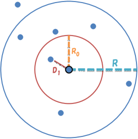
Figure 1: Range of View ($R$) and Separation($R_{0}$).

Some other essential parameters appearing in our BOIDS simulations and the setup are also explicitly given as follows.

• Field of simulations: Three dimensional open space without any gravity or any air resistance. Moreover, there is no wall and no ground surface.

• The number of agents in the flock: The system size of simulations is $N=100$

• Initial condition on the speed of each agent: $1<speed<8$.

• Initial condition on the location of each agent: All agents are distributed in a sphere with radius $L=180$.

• The shape and the range of each agent’s view: A sphere with radius $R=200$.

• The shape and the range of separation: A sphere with radius $R_{0}=20$.

For the above setting of the parameters, we shall implement two types of programming codes. One is a programing code for a single simulation (‘SS’ for short), and another code is for multiple simulations (‘MS’ for short). The SS runs in the GUI (graphical user interface) and it shows us a shape of the flock in real time, whereas the MS enables us to carry out a number of simulations with different initial conditions.

3.2 Typical four aggregations

By controling the three essential interactions, namely, ‘Cohesion’, ‘Alignment’ and ‘Separation’ mentioned above, we obtain four different aggregations having different collective behaviours. Each behavour of the aggregations is monitored (observed) by the SS. To specify the aggregation process of the flocks, we define the update rule of the vector of movement for each agent by

$$\mbox{\boldmath$v$}(t+1) = \frac{P_{0}\mbox{\boldmath$V$}_{\rm Cohesion}(t)+P_{1}\mbox{\boldmath$V$}_{\rm Alignment}(t)+P_{2}\mbox{\boldmath$V$}_{\rm Separation}(t)+P_{3}\mbox{\boldmath$v$}(t)}{|P_{0}\mbox{\boldmath$V$}_{\rm Cohesion}(t)+P_{1}\mbox{\boldmath$V$}_{\rm Alignment}(t)+P_{2}\mbox{\boldmath$V$}_{\rm Separation}(t)+P_{3}\mbox{\boldmath$v$}(t)|}$$ (4)

where $t$ means the time step of the update and $|\mbox{\boldmath$A$}|$ denotes the $L_{1}$-norm of a vector $A$. $\mbox{\boldmath$V$}_{\rm Cohesion}$ is a vector pointing to the center of mass from each agent’s position. $\mbox{\boldmath$V$}_{\rm Alignment}$ denotes a vector to be obtained by averaging over the velocities of all agents. $\mbox{\boldmath$V$}_{\rm Separation}$ means a vector pointing to the direction of the movement of each agent to be separated from her (or his) nearest neighbouring mate. Therefore, the aggregation of the flock is completely specified by the weights of the above vectors, namely, $\mbox{\boldmath$P$}\equiv(P_{0},P_{1},P_{2},P_{3})$. Among all possible combinations of these weights $P$, we shall pick up typical four cases. Each property and the shape of each aggregation are explained as follows.

• Case 1 (Crowded Aggregation): The aggregation obtained by controlling the interaction of ‘Cohesion’ much stronger than the others, namely, $\mbox{\boldmath$P$}=(1,0,0,1)$.

• Case 2 (Spread Aggregation): The aggregation obtained by controlling the interaction of ‘Separation’ much stronger than the others, namely, $\mbox{\boldmath$P$}=(0,0,1,1)$.

• Case 3 (Synchronized Aggregation): The aggregation obtained by controlling the interaction of ‘Alignment’ much stronger than the others, namely, $\mbox{\boldmath$P$}=(0,1,1,1)$.

• Case 4 (Flock Aggregation): This aggregation obtained by adjusting every interactions appropriately, namely, $\mbox{\boldmath$P$}=(1,5,1.5.1)$.

Using the MS, we simulate each aggregation for $200$ times for different initial conditions. In each simulation, we measure the angular distribution and then the value of $\gamma$ is calculated. The number of crash is also updated when the coordinate of each agent is identical to (is shared with) the other agents. We start each measurement from the time point at which the total amount of the change in every agent’s speed is close to $0$ through the 80 turns of the update. In the next section, we explain the details of the result.

4 Results

In association with the each aggregation, we evaluate the $\gamma$-value with standard deviation and the average number of crashes for 200 independent runs of the BOIDS simulations. In following, we summarize the results.

• Case 1 (Crowded Aggregation): The typical behaviour of the flock and the angular distribution are shown in the upper left panel in Figure 2 and Figure 3, respectively. The $\gamma$-value is $0.333$ with standard deviation $0.083$ and the average number of crashes is $2091.74$.

• Case 2 (Spread Aggregation): The typical behaviour of the flock and the angular distribution are shown in the upper right panel in Figure 2 and Figure 3, respectively. The $\gamma$-value is $0.315$ with standard deviation $0.258$ and the average number of crashes is $0$.

• Case 3 (Synchronized Aggregation): The typical behaviour of the flock and the angular distribution are shown in the lower left panel in Figure 2 and Figure 3, respectively. The $\gamma$-value is $0.300$ with standard deviation $0.281$ and the average number of crashes is $0$.

• Case 4 (Flock Aggregation): The typical behaviour of the flock and the angular distribution are shown in the lower right panel in Figure 2 and Figure 3, respectively. The $\gamma$-value is $0.744$ with standard deviation $0.124$ and the average number of crashes is $0$.

 

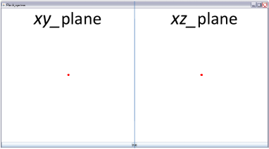
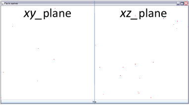
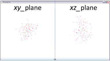
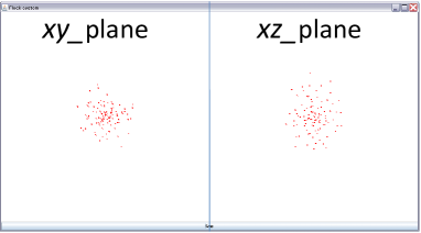
Figure 2: From the upper left to the lower right, snapshots of the typical behaviour for ‘Crowded Aggregation’, ‘Spread Aggregation’, ‘Synchronized Aggregation’ and ‘Flock Aggregation’ (the projections to the $xy$- and $xz$-planes) are shown.

 

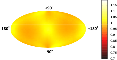
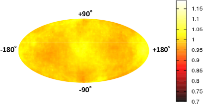
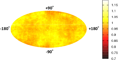
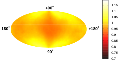
Figure 3: From the upper left to the lower right, angular density of the Case 1 ( ‘Crowded Aggregation’), the Case 2 (‘Spread Aggregation’), the Case 3 (‘Synchronized Aggregation’) and the Case 4 (‘Flock Aggregation’) are shown. The spatial symmetry in the Case 4 is apparently broken (the anisotropy emerges).

The aggregation of Case 4 (‘Flock Aggregation’) has the highest $\gamma$-value among the four cases and its angular density clearly shows a lack of nearest neighbours along the direction of flock’s motion leading to an anisotropy. For all aggregations except for the Case 4, the $\gamma$-values are lower than $\gamma_{isotropy}=1/3$, namely, they have no anisotropy. From these results, we find that BOIDS computer simulations having appropriate weights $P$ shows anisotropy structures as real flocks exhibit. It is also revealed that one can evaluate to what extent an arbitrary flock simulation is close to real flocks through the $\gamma$-value.

From the results obtained here, we might have another question, namely, it is important for us to answer the question such as whether the aggregation having a higher $\gamma$-value than the Case 4 seems to be more realistic than the Case 4 or not. To answer the question, we carry out the simulations of the flock aggregation which has a higher $\gamma$-value (Case 5) than the Case 4. The results are summarized as follows.

• Case 5 (Crowded Aggregation): The angular distribution is shown in Figure 4. The $\gamma$-value is $0.931$ with standard deviation $0.02$ and the average number of crashes is $570.6$.

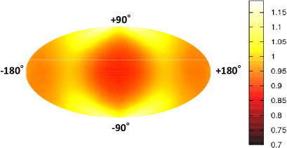
Figure 4: The angular density for the aggregation (Case 5) having a higher $\gamma$-value than the Case 4.

Obviously, the above aggregation has the highest $\gamma$-value leading to the strongest anisotropy among the five cases. However, it is hard for us to say that it is an optimal flock because the number of cashes is also the highest ($570$ times) and to make matter worse, the number itself is apparently outstanding. This result tells us that an aggregation having much stronger anisotropic structures is not always a better flock.

The above result is reasonably accepted because the $\gamma$-value is calculated from the angular distribution of nearest neighbours without any concept of the distance between agents. Therefore, the flock having a dense network might have highly risks of crashes more than the sparse network. For this reason, in order to judge whether a given aggregation has a better flock behaviour or not, we should use the other criteria which take into account the distance between nearest neighbours.

Inspired by the empirical data analysis by Ballerini et al [5], we finally calculate the $\gamma$-value as a function of the order of the neighbour. The result is shown in Figure 5.

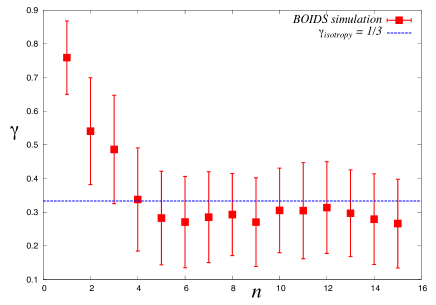
Figure 5: The $\gamma$-value as a function of the neighbour $n$ in the real flock.

In this figure, $n$ denotes the order of the neighbour, for instance, $n=1$ or $n=2$ means the nearest neighbour, the next nearest neighbour, respectively. The figure shows a similar behaviour to the corresponding plot in the reference [5], that is, the $\gamma$-values monotonically decrease as $n$ increases and they converge to $\gamma_{isotropy}=1/3$ beyond $n\simeq 6$. This result might be a justification to conclude that our BOIDS simulations having appropriate weight vectors $P$ actually simulate a realistic flock.

5 Concluding remarks

In this paper, we showed that the anisotropy observed in the empirical data analysis [5] also emerges in our BOIDS simulations having appropriate weight vectors $P$. From the $\gamma$-value we calculated, one can judge wheter an optional aggregation behaves like a real flock or not. The system of flocks is spatially ‘symmetric’ for $\gamma=\gamma_{isotropy}=1/3$, whereas the symmetry is ‘spontaneously’ broken for $\gamma>\gamma_{isotropy}$. We found from the behaviour of ‘order parameter’ $\gamma$ that this ‘spontaneous symmetry breaking’ is nothing but the emergence of anisotropy.

As well-known, there are some conjectures on the origin of the emergence of anisotropy. For instance, the effect of bird’s vision is one of the dominant hypotheses. In fact, real starlings have lateral visual axes and each of the starlings has a blind rear sector [8]. If all individuals in the flock move to avoid their nearest neighbours which are hidden in their blind sectors, the effect of the blind sector is more likely to be a factor to emerge the anisotropy of nearest neighbours in the front-rear directions. However, our result proved that this hypothesis is NOT ALWAYS correct because agents in our simulation have no blind sector of their views. Nevertheless, we found that our flock aggregation has an anisotropy of the nearest neighbours. The result means that the agent’s blind as an effect of vision is not necessarily required to produce the anisotropy and much more essential factor for the anisotropy is the best possible combinations of three essential interactions in the BOIDS.

We hope that these results might help us to consider the relevant link between BOIDS simulations and empirical evidence from real world.

References

- [1] Iwao Bialynicki-Birula and Iwona Bialynicka-Birula, Modeling Reality: How computers mirror life, Oxford University Press (2004).
- [2] D.P. Landau and K. Binder, A Guide to Monte Carlo Simulations in Statistical Physics, Cambridge University Press (2000).
- [3] C.W. Reynolds, Flocks, Herds, and Schools: A Distributed Behavioral Model, Computer Graphics 21, pp.25-34 (1987).
- [4] http://www.red3d.com/cwr/boids/
- [5] M. Ballerini, N. Cabibbo, R. Candelier, A. Cavagna, E. Cisbani, I. Giardina, V. Lecomte, A. Orlandi, G. Parisi, A. Procaccini, M. Viale and V. Zdravkovic, Interaction Rulling Animal Collective Behaviour Depends on Topological raher than Metric Distance, Evidence from a Field Study, Proceedings of the National Academy of Sciences USA 105, pp.1232-1237 (2008).
- [6] A. Cavagna, I. Giardina, A. Orlandi, G. Parisi, A. Procaccini, M. Viale and V. Zdravkovic, The STARFLAG handbook on collective animal behaviour: Part II, empirical methods, Animal Behaviour 76, Issue 1, pp237-248 (2008).
- [7] J.M. Cullen, E. Shaw and H.B. Baldwin, Methods for measuring the three dimensional structure of fish schools, Animal Behaviour 13, pp. 534-543 (1965).
- [8] G.R. Martin, The eye of a passeriform bird, the European starling (Sturnus vulgaris): eye movement amplitude, visual fields and schematic optics, J. Comp. Physiol. A 159, pp. 545-557 (1986).