Topological degree in analysis of canard-type trajectories in 3-D systems

Alexei Pokrovskii

Department of Applied Mathematics

University College Cork, Ireland

Dmitrii Rachinskii

Department of Applied Mathematics

University College Cork, Ireland

Vladimir Sobolev

Department of Differential Equations and Control Theory

Samara State University, Russia

Andrew Zhezherun

Department of Civil and Environmental Engineering

University College Cork, Ireland

(Communicated by )

1. Introduction

Topological degree [4, 8] is one of the principal toolboxes of the modern theory of nonlinear dynamical systems. The range of applications of this toolbox is rapidly growing, see, for instance, [5]. In this paper we discuss a new, to the best of our knowledge, scheme of applying topological degree to the analysis of canard-type trajectories.

If $W\colon\mathord{\mathbb{R}}^{d}\mapsto\mathord{\mathbb{R}}^{d}$ is a continuous mapping, $\Omega\subset\mathord{\mathbb{R}}^{d}$ is a bounded open set, and $y\in\mathord{\mathbb{R}}^{d}$ does not belong to the image $W(\partial\Omega)$ of the boundary $\partial\Omega$ of $\Omega$, then the symbol $\deg(W,\Omega,y)$ denotes the topological degree [4] of $W$ at $y$ with respect to $\Omega$. If $0\not\in W(\partial\Omega)$, then the integer number $\gamma(W,\Omega)=\deg(W,\Omega,0)$, called the rotation of the vector field $W$ at $\partial\Omega$, is well defined. A detailed description of properties of the number $\gamma(W,\Omega)$ can be found, for example, in [8]. In particular, if $\mathrm{id}$ denotes the identity mapping, $\mathrm{id}(x)\equiv x$, then the number $\gamma(\mathrm{id}-W,\Omega)$ measures the algebraic number of fixed points of the mapping $W$ in $\Omega$.

We will use this tool to investigate canard-type periodic trajectories of singularly perturbed differential equations. Let us recall some related terminology. Consider the slow-fast system

$$\dot{x} =f(x,y,z),$$

$$\dot{y} =g(x,y,z),$$ (1)

$$\varepsilon\dot{z} =h(x,y,z),$$

where $x$, $y$, $z$ are scalar functions of time, $\varepsilon$ is a small positive parameter, and $f$, $g$, $h$ are scalar functions. The subset

$$S=\left\{(x,y,z)\in\mathord{\mathbb{R}}^{3}\colon h(x,y,z)=0\right\}$$

of the phase space is called a slow surface of the system (1): on this surface the derivative $\dot{z}$ of the fast variable is zero. Moreover, a part of $S$ where

$$\frac{\partial h}{\partial z}(x,y,z)<0\qquad\left(\frac{\partial h}{\partial z}(x,y,z)>0\right)$$

is called attractive (repulsive, respectively). A line $L\subset S$ which separates attractive and repulsive parts of $S$ will be called a turning line. In what follows, we suppose the turning line to be smooth. Trajectories which at first pass along, and close to, an attractive part of $S$ and then continue for a while along the repulsive part of $S$ are called canards or duck-trajectories [2].

In the paper, we focus our attention on periodic canards in singularly perturbed picewise linear systems, or more specifically, in a special case of (1) with $h(x,y,z)=x+{\mathopen{|}z\mathclose{|}}$. This choice has a number of reasons. From the methodological point of view, piecewise linear systems are convenient because they are integrable. Furthermore, such systems are used extensively in the modelling of a wide range of physical processes and have applications in electrical circuits [7, 3, 6], flight control [14], chemical processes control [13] and neural subsystems with control behavior [9]. The piecewise linearity may be due to nonlinear elements such as saturation or may result from linearization about various operating points of a nonlinear plant. For example, the McKean model is a piecewise linear caricature of the FitzHugh-Nagumo model [10].

The main mathematical reason to consider the existence of periodic canards for this class of differential systems is that they (together with classical canards) are mathematical explanations of the limit behaviour of periodic solutions of a family of differential equations. However, the traditional methods of the “chasse au canard” are adapted for sufficiently smooth systems, and we consider the use of topological methods in the case of Lipschitzian nonlinearities as a dire necessity (continuous piecewise linear functions satisfy the Lipschitz condition, see, for example, [6]).

Note that system (1) has a vector slow variable $(x,y)$, and it is known that the existence conditions for canards in systems with scalar and vector slow variables have a vital difference. In the scalar case it is necessary to have an additional parameter in the system under consideration, which is demonstrated in [15, 12] where piecewise linear systems on the plane are studied. The canard then exists only for a small range of values of the parameter. In the vector case such a parameter is not required, hence the system (1), under some assumptions about the right hand side given in the next section, always has a canard. Below we show that (1) also has a periodic canard if some additional assumptions are made.

2. Main result

In this section we formulate the main existence result for topologically stable canard type periodic trajectories, using a simple example.

Consider a system of ordinary differential equations:

$${\begin{array}[]{rl}\dot{x}&{}=f(x,y,z),\\[3.0pt] \dot{y}&{}=g(x,y,z),\\[3.0pt] \varepsilon\dot{z}&{}=x+{\mathopen{|}z\mathclose{|}},\end{array}}$$ (2)

with the additional assumptions described below.

The slow surface of the system consists of two half-planes, an attractive half-plane $P_{a}$ and a repulsive half-plane $P_{r}$:

$$P_{a} =\{(x,y,x)\colon x<0\},$$ (3)

$$P_{r} =\{(x,y,-x)\colon x<0\},$$ (4)

together with the turning line

$$L=\{(0,y,0)\}.$$ (5)

We consider auxiliary equations

$${\begin{array}[]{l}\dot{x}=f_{a}(x,y)=f(x,y,x),\\[3.0pt] \dot{y}=g_{a}(x,y)=g(x,y,x),\end{array}}$$ (6)

and

$${\begin{array}[]{l}\dot{x}=f_{r}(x,y)=f(x,y,-x),\\[3.0pt] \dot{y}=g_{r}(x,y)=g(x,y,-x),\end{array}}$$ (7)

which describe the dynamics near the slow half-planes (3) and (4) in the limit $\varepsilon\to 0$.

Assumption 1.

The functions $f$ and $g$ in the right-hand side of (2) are globally bounded and globally Lipschitz continuous with a Lipschitz constant $\lambda$:

$${\mathopen{|}f(x,y,z)\mathclose{|}},{\mathopen{|}g(x,y,z)\mathclose{|}}<M.$$ (8)

Assumption 2.

The following relationships hold:

$$f(0,0,0)=0,\quad g(0,0,0)>0,\quad y\cdot f(0,y,0)<0.$$

An important role is played below by the solutions of (6) and (7). Denote by $w^{*}_{a}(t)=(x^{*}_{a}(t),y^{*}_{a}(t))$ the solution of the system (6), satisfying the initial condition $x(0)=y(0)=0$, and by $w^{*}_{r}(t)=(x^{*}_{r},y^{*}_{r})$ the solution of the system (7), satisfying the same initial condition.

Assumption 2 ensures the existence of a finite time interval $(T_{a},T_{r})\ni 0$ such that

$$x^{*}_{a}(t)<0\mbox{ for }T_{a}<t<0,\quad x^{*}_{r}(t)<0\mbox{ for }0<t<T_{r}.$$

Assumption 2 also implies strict limitation on the possible location of canards of system (2), which should follow closely the attractive half-plane (3) for a certain interval $t_{a}<t<0$, and then move along the repulsive half-plane (4) for $0<t<t_{r}$. Any such canard must first follow the curve

$$\Gamma_{a}=\{(x^{*}_{a}(t),y^{*}_{a}(t),x^{*}_{a}(t))\}\subset P_{a}$$ (9)

for negative times, and then the curve

$$\Gamma_{r}=\{(x^{*}_{r}(t),y^{*}_{r}(t),-x^{*}_{r}(t))\}\subset P_{r}$$ (10)

for positive times, passing near the origin, where the two curves meet at $t=0$. Using standard tools, see [1, 11], it is easy to see that for any time interval $[t_{a},t_{r}]\subset(T_{a},T_{r})$ with $t_{a}<0<t_{r}$ such a canard exists for every sufficiently small $\varepsilon>0$.

The question whether there exist periodic canards is less obvious. The above argument shows that a periodic canard should have a segment of fast motion from a small neighborhood of some point of the curve $\Gamma_{r}$ to a small neighborhood of the curve $\Gamma_{a}$; this fast motion is, consequently, almost vertical (i.e., almost parallel to the $z$ axis). More precisely, if there is a limit of periodic canards as $\varepsilon\to 0$, then the limiting closed curve has necessarily a vertical segment connecting $\Gamma_{r}$ and $\Gamma_{a}$. The next assumption ensures a possibility of such vertical jumps.

Assumption 3.

The trajectories $w^{*}_{a}(t)$ and $w^{*}_{r}(t)$ of systems (6) and (7) intersect, that is, there exist $\tau$ and $\sigma$ such that

$$x^{*}_{a}(\tau)=x^{*}_{r}(\sigma)=x^{*},\quad y^{*}_{a}(\tau)=y^{*}_{r}(\sigma)=y^{*}$$

with

$$T_{a}<\tau<0<\sigma<T_{r}.$$

Assumption 4.

The intersection is transversal, that is

$$A=f_{a}(x^{*},y^{*})g_{r}(x^{*},y^{*})-f_{r}(x^{*},y^{*})g_{a}(x^{*},y^{*})\not=0.$$

Assumptions 3–4 are illustrated on Fig. 1.

Figure 1. Solutions $w^{*}_{a}(t)$ and $w^{*}_{r}(t)$.

The following theorem states the existence of periodic canard in the system (2) under the Assumptions 1–4.

Theorem 1.

For every sufficiently small $\varepsilon>0$ there exists a periodic solution of system (2). The minimal period $T_{\min}$ of this solution approaches $\sigma-\tau$ as $\varepsilon\to 0$.

It will also be shown that the periodic canard passes through a small neighbourhood of the point $(x^{*},y^{*},0)$, with the diameter of this neighbourhood going to zero as $\varepsilon$ goes to zero.

Below we discuss the main ideas behind the proof of this theorem. The proof itself, which is divided into several technical propositions and lemmas, will be provided in the next section.

Denote by

$$w_{a}(t,t_{0},x_{0},y_{0})=(x_{a}(t,t_{0},x_{0},y_{0}),y_{a}(t,t_{0},x_{0},y_{0}))$$

the solution of system (6) with the initial condition

$$x(t_{0})=x_{0},\quad y(t_{0})=y_{0}.$$

Similarly, denote by

$$w_{r}(t,t_{0},x_{0},y_{0})=(x_{r}(t,t_{0},x_{0},y_{0}),y_{r}(t,t_{0},x_{0},y_{0}))$$

the solution of system (7) with the same initial condition

$$x(t_{0})=x_{0},\quad y(t_{0})=y_{0}.$$

Consider a small vicinity of the point $(x^{*},y^{*})$. Since the intersection between $\Gamma_{a}$ and $\Gamma_{r}$ is transversal according to Assumption 4, the numbers $u(x,y)$ and $v(x,y)$ may be defined in this vicinity by

$$w_{a}(u(x,y),0,x,y)\in\Gamma_{r},\quad w_{r}(v(x,y),0,x,y)\in\Gamma_{a}.$$

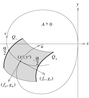
Figure 2. The set $\Pi(\alpha)$ on the plane $(x,y)$.

Using the coordinates $u(x,y)$ and $v(x,y)$ we introduce for a sufficiently small $\alpha>0$ a ‘parallelogram’ set $\Pi(\alpha)$, illustrated on Fig. 2:

$$\Pi(\alpha)=\{x,y\colon{\mathopen{|}u(x,y)\mathclose{|}},{\mathopen{|}v(x,y)\mathclose{|}}<\alpha/2\}.$$ (11)

Also introduce the notation for the two ‘sides’ of this parallelogram:

$$Q_{-} {}=\{x,y\colon v(x,y)=+\alpha/2\operatorname{sgn}A,{\mathopen{|}u(x,y)\mathclose{|}}\leq\alpha/2\},$$

$$Q_{+} {}=\{x,y\colon v(x,y)=-\alpha/2\operatorname{sgn}A,{\mathopen{|}u(x,y)\mathclose{|}}\leq\alpha/2\}.$$

Denote by

$$w_{\varepsilon}(t,x_{0},y_{0})=(x_{\varepsilon}(t,x_{0},y_{0}),y_{\varepsilon}(t,x_{0},y_{0}),z_{\varepsilon}(t,x_{0},y_{0}))$$ (12)

the solution of the system (2) with the initial condition

$$x(\tau)=x_{0},\quad y(\tau)=y_{0},\quad z(\tau)=0,$$

with $(x_{0},y_{0})\in\Pi(\alpha)$.

In our assumptions, the solution $w_{\varepsilon}(t,x_{0},y_{0})$ first rapidly approaches the attractive half-plane $P_{a}$ defined in (3), and then follows $P_{a}$ until $t\approx 0$. The possible subsequent behaviors of the solution are the following:

1. The solution stays close to the attractive part of the slow surface for $t\leq\delta$, where $\delta>0$.

2. The solution begins to rapidly increase in the $z$ direction around $t\approx 0$.

3. The solution follows the repulsive half-plane $P_{r}$ defined in (4), until a moment $t^{*}$. Moreover, for positive $t<t^{*}$ it follows the curve $\Gamma_{r}$. After the moment $t^{*}$ the solution may begin to rapidly increase in the $z$ direction, or it may fall down back to the attractive part of the slow surface.

To distinguish between these cases, we define the time moment

$$s_{\varepsilon}(x_{0},y_{0})=\min(\{T_{r}\}\cup\{t\colon\tilde{t}(x_{0},y_{0})+\rho\leq t\leq T_{r}\colon z_{\varepsilon}(t,x_{0},y_{0})\leq 0\}),$$ (13)

where $\tilde{t}(x_{0},y_{0})$ is a time moment close to zero, which is associated with the solution $w_{a}(t,\tau,x_{0},y_{0})$ and which will be introduced in the next section, and $\rho>0$ is a sufficiently small number chosen together with $\alpha$.

Using the moment $s_{\varepsilon}(x_{0},y_{0})$, we define an auxiliary mapping $W_{\varepsilon}$ of the parallelogram $\Pi(\alpha)$ into the plane $(x,y)$. The definition is divided into the following four cases:

Case 1. If

$$\sigma-\alpha<s_{\varepsilon}(x_{0},y_{0})<\sigma+\alpha,$$

then

$$W_{\varepsilon}(x_{0},y_{0})=(x_{\varepsilon}(s_{\varepsilon},x_{0},y_{0}),y_{\varepsilon}(s_{\varepsilon},x_{0},y_{0})).$$

If we identify the plane $(x,y)$ with the two-dimensional subspace

$$P_{0}=\{(x,y,0)\colon x,y\in\mathord{\mathbb{R}}\}$$

of the phase space of system (2), then in Case 1 the value $W_{\varepsilon}(x_{0},y_{0})$ coincides with the intersection of the trajectory (12) with $P_{0}$, as long as the corresponding intersection time is close to $\sigma$.

Case 2. If

$$\alpha\leq{\mathopen{|}s_{\varepsilon}(x_{0},y_{0})-\sigma\mathclose{|}}<2\alpha,$$

then

$$W_{\varepsilon}(x_{0},y_{0})=\frac{2\alpha-{\mathopen{|}s_{\varepsilon}-\sigma\mathclose{|}}}{\alpha}(x_{\varepsilon}(s_{\varepsilon},x_{0},y_{0}),y_{\varepsilon}(s_{\varepsilon},x_{0},y_{0}))+\frac{{\mathopen{|}s-\sigma\mathclose{|}}-\alpha}{\alpha}w^{*}_{r}(s_{\varepsilon}).$$

This means that $W_{\varepsilon}(x_{0},y_{0})$ is a continuous convex combination of the intersection of the trajectory (12) with $P_{0}$ and the point $w^{*}_{r}(s_{\varepsilon})$ as long as the discrepancy ${\mathopen{|}s_{\varepsilon}-\sigma\mathclose{|}}$ between the corresponding intersection moment $s_{\varepsilon}$ and $\sigma$ in the the range from $\alpha$ to $2\alpha$. Moreover, if the discrepancy equals $\alpha$, then the definition is consistent with Case 1; if the intersection moment equals $\sigma\pm 2\alpha$, then $W_{\varepsilon}$ coincides with $w^{*}_{r}(\sigma\pm 2\alpha)$.

Case 3. If

$$s_{\varepsilon}(x_{0},y_{0})\geq\sigma+2\alpha,$$

then

$$W_{\varepsilon}(x_{0},y_{0})=w^{*}_{r}(\sigma+2\alpha).$$

Case 4. If

$$s_{\varepsilon}(x_{0},y_{0})\leq\sigma-2\alpha,$$

then

$$W_{\varepsilon}(x_{0},y_{0})=w^{*}_{r}(\sigma-2\alpha).$$

For small $\varepsilon$, $\alpha$ and $\rho$ the time moment $s_{\varepsilon}(x_{0},y_{0})$ depends continuously on $(x_{0},y_{0})$, therefore the operator $W_{\varepsilon}(x_{0},y_{0})$ is also continuous with respect to $(x_{0},y_{0})$. We will show that if $(x_{0},y_{0})$ is a fixed point of $W_{\varepsilon}$, then Case 1 takes place, so the triple $(x_{0},y_{0},0)$ defines a periodic solution of (2) with the period $s_{\varepsilon}-\tau$ close to $\sigma-\tau$.

We also prove that the images of the parallelogram sides $Q_{-}$ and $Q_{+}$ are the points $w^{*}_{r}(\sigma+2\alpha)$ and $w^{*}_{r}(\sigma-2\alpha)$ correspondingly, and $u(W_{\varepsilon}(x_{0},y_{0}))\to 0$ as $\varepsilon\to 0$, thus the operator $W_{\varepsilon}$ is contracting along the $u$ coordinate, and stretching along the $v$ coordinate. Finally, the vector field rotation theory is used to obtain the relation

$$\gamma(\mathrm{id}-W_{\varepsilon},\Pi(\alpha))=\operatorname{sgn}A\not=0,$$

which implies the existence of a fixed point of the operator $W_{\varepsilon}$ in the set $\Pi(\alpha)$, thus proving the existence of a periodic canard.

3. Proof of Theorem 1

The proof consists of several parts. First, we formulate the properties of the solutions $w_{a}(t,x_{0},y_{0})=w_{a}(t,\tau,x_{0},y_{0})$ of the system (6) on the set $\Pi(\alpha)$. Secondly, we consider the behavior of the solution $w_{\varepsilon}(t,x_{0},y_{0})$ of the system (2) and establish the continuity of the time moment $s_{\varepsilon}(x_{0},y_{0})$ which was defined in (13) and thus the continuity of the operator $W_{\varepsilon}$ on $\Pi(\alpha)$. Finally, we calculate the rotation of the vector field $\mathrm{id}-W_{\varepsilon}$ on $\Pi(\alpha)$.

We will need the following auxiliary definitions.

Definition 1.

We say that $a$ is $\varepsilon$-close to $b$, if $a\to b$ as $\varepsilon\to 0$. $a$ is said to be $\varepsilon$-small, if it is $\varepsilon$-close to 0.

Consider a solution $w_{a}(t,x_{0},y_{0})$ of the auxiliary system (6) with the initial condition $(x(\tau),y(\tau))=(x_{0},y_{0})\in\Pi$.

Define the set

$$R=\{(x,y)\colon(x=0\wedge y\leq 0)\vee(x\leq 0\wedge y=0)\},$$

which is the union of the left half of the horizontal $x$ coordinate axis and the bottom half of the vertical $y$ coordinate axis. Consider all the time moments ${\mathcal{T}}(x_{0},y_{0})$ when the solution $w_{a}(t,x_{0},y_{0})$ intersects the set $R$:

$${\mathcal{T}}(x_{0},y_{0})=\{t\colon w_{a}(t,x_{0},y_{0})\in R\}.$$

Figure 3. The set ${\mathcal{T}}$ and the moment $\tilde{t}$.

Definition 2.

Let $\tilde{t}(x_{0},y_{0})$ be the moment from the set ${\mathcal{T}}(x_{0},y_{0})$ closest to zero, see Fig. 3:

$$\tilde{t}=\operatorname*{arg\,min}_{t\in{\mathcal{T}}(x_{0},y_{0})}{\mathopen{|}t\mathclose{|}}.$$

Below we sometimes omit the point $(x_{0},y_{0})$ and write simply $\tilde{t}$, in which case the arguments can be uniquely identified from the context.

Definition 3.

If $\tilde{t}(x_{0},y_{0})$ exists, and $x_{a}(\tilde{t},x_{0},y_{0})=0$ and $y_{a}(\tilde{t},x_{0},y_{0})<0$, then the solution $w_{a}(t,x_{0},y_{0})$ together with the point $(x_{0},y_{0})$ are called destabilizing. If $x_{a}(\tilde{t},x_{0},y_{0})<0$ and $y_{a}(\tilde{t},x_{0},y_{0})=0$, then the solution $w_{a}(t,x_{0},y_{0})$ and the point $(x_{0},y_{0})$ are called stabilizing.

This definition emphasizes the fact that the solution $w_{\varepsilon}(t,x_{0},y_{0})$ of the main equation (2) with a stabilizing initial condition will stay close to the attractive half-plane $P_{a}$ for some time after $t>0$, if $\varepsilon$ is sufficiently small; if initial condition is destabilizing, then $z_{\varepsilon}(t)$ will rapidly increase to infinity after $t>0$. The proof of this fact will be the subject of several propositions, all leading to Proposition 6.

Statement 1.

If $\alpha$ is sufficiently small, then the moment $\tilde{t}$ is defined for all $(x_{0},y_{0})\in\Pi$ and is continuous on $\Pi$ with respect to $(x_{0},y_{0})$.

Statement 2.

If $\alpha$ is sufficiently small, then a point $(x_{0},y_{0})\in\Pi$ is destabilizing if $A\cdot v(x_{0},y_{0})>0$, and stabilizing if $A\cdot v(x_{0},y_{0})<0$. In particular, $Q_{-}$ is destabilizing and $Q_{+}$ is stabilizing.

Statement 3.

Let $\alpha$ be sufficiently small. If $(x_{0},y_{0})$ is destabilizing, then $x_{a}(t)<0$ for $\tau\leq t<\tilde{t}$, and if $(x_{0},y_{0})$ is stabilizing, then $x_{a}(t)<0$ for $\tau\leq t\leq\delta(\alpha)$ where $\delta(\alpha)>\max_{\Pi}\{\tilde{t}(x_{0},y_{0})\}>0$ depends only on $\alpha$.

Statement 1 follows from the continuous dependence of $w_{a}$ on $(x_{0},y_{0})$ and from the fact that $w_{a}^{*}$ intersects the line $y=0$ transversally.

To prove Statements 2 and 3, we can consider the projection $d(t)$ of the difference between the trajectories $w_{a}(t,x_{0},y_{0})$ and $w_{a}^{*}(t)$ onto the normal vector for $w_{a}^{*}(t)$, $t\geq\tau$:

$$d(t)=(x_{a}(t)-x_{a}^{*}(t))g_{a}(x_{a}^{*}(t),y_{a}^{*}(t))-(y_{a}(t)-y_{a}^{*}(t))f_{a}(x_{a}^{*}(t),y_{a}^{*}(t)).$$

Then the variation of $d(t)$ satisfies the following initial value problem:

$$\dot{r}(t)=(\tfrac{\partial}{\partial x}f_{a}(x_{a}^{*}(t),y_{a}^{*}(t))+\tfrac{\partial}{\partial y}g_{a}(x_{a}^{*}(t),y_{a}^{*}(t)))r(t),\quad r(\tau)=1,$$

and the following equality holds for small $\Delta x_{0}=x_{0}-x_{*}$, $\Delta y_{0}=y_{0}-y_{*}$, $d_{0}=\Delta x_{0}g_{a}(x_{*},y_{*})-\Delta y_{0}f_{a}(x_{*},y_{*})$:

$$d(t)=r(t)d_{0}+o(\Delta x_{0})+o(\Delta y_{0}).$$

Therefore, if $d_{0}>0$, and $\Delta x_{0}$ and $\Delta y_{0}$ are small, then $d(t)>0$ for $\tau\leq t\leq T_{r}$. Assumption 4 provides that $d_{0}>0$ for $(x_{0},y_{0})\in Q_{-}$, and $d_{0}<0$ for $(x_{0},y_{0})\in Q_{+}$.

Denote $\omega=\varepsilon\ln\frac{T}{\varepsilon}$ with $T=-T_{a}+T_{r}$, $\omega>\varepsilon$ for sufficiently small $\varepsilon$.

Consider the solution $w_{\varepsilon}(t,x_{0},y_{0})$ defined by (12) with $(x_{0},y_{0})\in\Pi$.

Proposition 1.

The sets $z>-x+M\varepsilon$ and $z>x-M\varepsilon$ are invariant in the sense that once a trajectory enters them, it does not leave them. In particular, if $x_{0}<0$ and $z_{0}=0$, then $z_{\varepsilon}>x_{\varepsilon}-M\varepsilon$ for all $t\geq\tau$, and if additionally $z_{\varepsilon}(t_{0})>-x_{\varepsilon}+M\varepsilon$ for some $t_{0}$, then $z_{\varepsilon}(t)>0$ for all $t\geq t_{0}$.

Proof.

Denote $\varphi(t)=z(t)+x(t)$, $\psi(t)=z(t)-x(t)$. Then (2) together with assumption (8) imply that

$$\dot{\varphi}={} \dot{z}+\dot{x}=\frac{1}{\varepsilon}(x+{\mathopen{|}z\mathclose{|}})+f(x,y,z)\geq\frac{1}{\varepsilon}(x+z)-M=\frac{1}{\varepsilon}\varphi-M,$$

$$\dot{\psi}={} \dot{z}-\dot{x}=\frac{1}{\varepsilon}(x+{\mathopen{|}z\mathclose{|}})-f(x,y,z)\geq\frac{1}{\varepsilon}(x-z)-M=-\frac{1}{\varepsilon}\psi-M,$$

and by the theorem on differential inequalities,

$$\varphi(t)\geq\bar{\varphi}(t)=(\varphi_{0}-M\varepsilon)e^{\frac{t-t_{0}}{\varepsilon}}+M\varepsilon,$$

$$\psi(t)\geq\bar{\psi}(t)=(\psi_{0}+M\varepsilon)e^{-\frac{t-t_{0}}{\varepsilon}}-M\varepsilon,$$

with $\varphi_{0}=\varphi(t_{0})=z(t_{0})+x(t_{0})$. and $\psi_{0}=\psi(t_{0})=z(t_{0})-x(t_{0})$. If $\varphi_{0}>M\varepsilon$, then $\bar{\varphi}(t)>M\varepsilon$ and thus $z(t)>-x(t)+M\varepsilon$ for all $t\geq t_{0}$. Similarly, if $\psi_{0}>-M\varepsilon$, then $\bar{\psi}(t)>-M\varepsilon$, therefore $z(t)>x(t)-M\varepsilon$ for all $t\geq t_{0}$.

The second part of the proposition follows from the fact that the point $(x_{0},y_{0},0)$ with $x_{0}<0$ is in the set $z>x-M\varepsilon$, and if both $z>x-M\varepsilon$ and $z>-x+M\varepsilon$ hold, then $z>0$. ∎

Proposition 2.

Let $\varepsilon$ be sufficiently small. Denote

$$\hat{t}=\min(\{T_{r}\}\cup\{t>\tau\colon z_{\varepsilon}(t)=0\}),$$ (14)

and

$$t_{1}=\tau+\varepsilon\ln\Bigl{(}-\frac{x_{0}}{M\varepsilon}\Bigr{)}.$$ (15)

Then $t_{1}<\tau+\omega$, $\hat{t}>t_{1}$, and for $t_{1}\leq t\leq\hat{t}$:

$${\mathopen{|}z_{\varepsilon}(t)-x_{\varepsilon}(t)\mathclose{|}}<2M\varepsilon.$$

Proof.

According to Proposition 1, the solution $w_{\varepsilon}(t)$ does not leave the set $z-x>-M\varepsilon$, because $(x_{0},y_{0})\in\Pi$ and thus $z_{0}-x_{0}>0$. Therefore, it suffices to prove the relation $z_{\varepsilon}(t)-x_{\varepsilon}(t)<2M\varepsilon$ for $t_{1}\leq t\leq\hat{t}$.

First we prove that $z_{\varepsilon}(t)<0$ for $\tau<t\leq t_{1}$, which will imply $\hat{t}>t_{1}$. Note that $-MT<x_{0}<-M\varepsilon$, thus $t_{1}<\tau+\omega$. Assuming that $z(t)<0$, we get the following relations for $\psi=z-x$:

$$\dot{\psi}=\dot{z}-\dot{x}=\frac{1}{\varepsilon}(x-z)-f(x,y,z),$$

$$\dot{\psi}\geq-\frac{1}{\varepsilon}\psi-M,\quad\psi_{0}=z_{0}-x_{0}>M\varepsilon,$$ (16)

$$\dot{\psi}(t)\geq(\psi_{0}+M\varepsilon)e^{-\frac{1}{\varepsilon}(t-\tau)}-M\varepsilon=\psi^{(1)}(t).$$

The function $\psi^{(1)}(t)$ is decreasing, and

$$\psi^{(1)}(t_{1})=(\psi_{0}+M\varepsilon)\frac{M\varepsilon}{\psi_{0}}-M\varepsilon>0,$$

therefore $\dot{z}_{\varepsilon}=-\frac{1}{\varepsilon}\psi\leq-\frac{1}{\varepsilon}\psi^{(1)}<0$ for $\tau\leq t\leq t_{1}$, which proves that $z_{\varepsilon}(t)<0$ for $\tau<t\leq t_{1}$.

Now, similarly to (16), we write

$$\dot{\psi}\leq-\frac{1}{\varepsilon}\psi+M,$$

$$\dot{\psi}(t)\leq(\psi_{0}-M\varepsilon)e^{-\frac{1}{\varepsilon}(t-\tau)}+M\varepsilon=\psi^{(2)}(t),$$

$$\psi^{(2)}(t_{1})=(\psi_{0}-M\varepsilon)\frac{M\varepsilon}{\psi_{0}}+M\varepsilon<2M\varepsilon,$$

thus for $t\geq t_{1}$:

$$z_{\varepsilon}(t)-x_{\varepsilon}(t)\leq\psi^{(2)}(t)<2M\varepsilon.$$

This inequality holds while $z_{\varepsilon}(t)$ satisfies the equation $\dot{z}=\frac{1}{\varepsilon}(x-z)$, i.e. while $t\leq\hat{t}$. ∎

As before, $(x_{a},y_{a})$ will denote the solution of the system (6) with the initial condition $x(\tau)=x_{0}$, $y(\tau)=y_{0}$.

Proposition 3.

If $\varepsilon$ is sufficiently small, then the following inequalities hold for $\tau\leq t\leq\hat{t}$:

$${\mathopen{|}x_{\varepsilon}(t)-x_{a}(t)\mathclose{|}},{\mathopen{|}y_{\varepsilon}(t)-y_{a}(t)\mathclose{|}}\leq L\omega,$$

where $L=5Me^{4\lambda T}$.

Proof.

The moment $t_{1}$ defined by (15) in Proposition 2 is $\omega$-close to $\tau$, thus

$${\mathopen{|}x_{\varepsilon}(t_{1})-x_{a}(t_{1})\mathclose{|}}\leq{\mathopen{|}x_{\varepsilon}(t_{1})-x_{0}\mathclose{|}}+{\mathopen{|}x_{a}(t_{1})-x_{0}\mathclose{|}}\leq 2M\omega,\quad{\mathopen{|}y_{\varepsilon}(t_{1})-y_{a}(t_{1})\mathclose{|}}\leq 2M\omega.$$

Denote $\psi(t)={\mathopen{|}x_{\varepsilon}(t)-x_{a}(t)\mathclose{|}}+{\mathopen{|}y_{\varepsilon}(t)-y_{a}(t)\mathclose{|}}$, $t\geq t_{1}$. Using (2) and (6) together with Assumption 1 and Proposition 2, we obtain

$$D_{R}{\mathopen{|}x_{\varepsilon}-x_{a}\mathclose{|}}\leq{\mathopen{|}f(x_{\varepsilon},y_{\varepsilon},x_{\varepsilon})-f(x_{a},y_{a},x_{a})\mathclose{|}}+2\lambda M\varepsilon\leq 2\lambda{\mathopen{|}x_{\varepsilon}-x_{a}\mathclose{|}}+\lambda{\mathopen{|}y_{\varepsilon}-y_{a}\mathclose{|}}+2\lambda M\varepsilon,$$

$$D_{R}{\mathopen{|}y_{\varepsilon}-y_{a}\mathclose{|}}\leq{\mathopen{|}g(x_{\varepsilon},y_{\varepsilon},x_{\varepsilon})-g(x_{a},y_{a},x_{a})\mathclose{|}}+2\lambda M\varepsilon\leq 2\lambda{\mathopen{|}x_{\varepsilon}-x_{a}\mathclose{|}}+\lambda{\mathopen{|}y_{\varepsilon}-y_{a}\mathclose{|}}+2\lambda M\varepsilon,$$

where $D_{R}$ denotes the right derivative. Therefore

$$D_{R}\psi(t)\leq 4\lambda\psi(t)+4\lambda M\varepsilon,\quad\psi(t_{1})\leq 4M\omega.$$

and by the theorem on differential inequalities,

$$\psi(t)\leq(4M\omega+M\varepsilon)e^{4\lambda(t-t_{1})}-M\varepsilon\leq L\omega.$$

for $t_{1}\leq t\leq\hat{t}$. ∎

Proposition 4.

If $(x_{0},y_{0})$ is destabilizing and $\varepsilon$ is sufficiently small, then the solution $(x_{\varepsilon},y_{\varepsilon},z_{\varepsilon})$ reaches $z=0$ at the moment $\hat{t}$ which is $\varepsilon$-close to $\tilde{t}(x_{0},y_{0})$, and $z_{\varepsilon}(t)>0$ for all $t>\hat{t}$.

Proof.

Denote $\tilde{y}=y(\tilde{t})<0$, $\tilde{f}=f(0,\tilde{y},0)>0$, $\tilde{g}=g(0,\tilde{y},0)$. Consider a small vicinity $\Omega$ of the point $(0,\tilde{y},0)$:

$$\Omega=\{(x,y,z)\colon{\mathopen{|}x\mathclose{|}},{\mathopen{|}z\mathclose{|}},{\mathopen{|}y-\tilde{y}\mathclose{|}}\leq\delta\}$$

Due to the continuity of $f$ and $g$ we can select a sufficiently small $\delta$ such that $\tilde{f}/2<f(x,y,z)<2\tilde{f}$, and ${\mathopen{|}g(x,y,z)\mathclose{|}}<2\max\{\tilde{f},{\mathopen{|}\tilde{g}\mathclose{|}}\}$ for all $(x,y,z)\in\Omega$. Denote

$$\Delta\tilde{t}=\delta/(2\max\{\tilde{f},{\mathopen{|}\tilde{g}\mathclose{|}}\}),\quad\tilde{x}=x_{a}(\tilde{t}-\Delta\tilde{t})<0.$$

Then $(x_{a}(t),y_{a}(t),x_{a}(t))\in\Omega$ for $\tilde{t}-\Delta\tilde{t}\leq t\leq\tilde{t}+\Delta\tilde{t}$, $x_{a}(t)$ is increasing on this interval, and Statement 3 implies that

$$x_{a}(t)\leq\tilde{x}\mbox{ for }\tau\leq t\leq\tilde{t}-\Delta\tilde{t}.$$ (17)

First we will prove that $\hat{t}$ is $\varepsilon$-close to $\tilde{t}$. Let $\Delta t=4L\omega/\tilde{f}<\Delta\tilde{t}$ for sufficiently small $\varepsilon$. We have

$$x_{a}(\tilde{t}-\Delta t)<-2L\omega,\quad x_{a}(\tilde{t}+\Delta t)>2L\omega.$$ (18)

Consider the interval $I=\{t\colon t_{1}\leq t\leq\tilde{t}-\Delta t\}$. Inequalities (17), (18) together with the fact that $x_{a}(t)$ is increasing for $\tilde{t}-\Delta\tilde{t}\leq t\leq\tilde{t}-\Delta t$ imply that $x_{a}(t)<-2L\omega$ for $t\in I$. Applying Propositions 2 and 3, we obtain

$$z_{\varepsilon}(t)<x_{\varepsilon}(t)+2M\varepsilon<x_{a}(t)+L\omega+2M\varepsilon<0\mbox{ for }t\in I,$$

therefore $z_{\varepsilon}(t)<0$ for $\tau<t\leq\tilde{t}-\Delta t$.

Now suppose that $z_{\varepsilon}(t)<0$ for $\tilde{t}-\Delta t\leq t\leq\tilde{t}+\Delta t$. Then Propositions 2 and 3 will hold on this interval, and (18) will imply that

$$z_{\varepsilon}(\tilde{t}+\Delta t)>x_{\varepsilon}(\tilde{t}+\Delta t)-2M\varepsilon>x_{a}(\tilde{t}+\Delta t)-L\omega-2M\varepsilon>0.$$

This contradiction proves that $\hat{t}$ lies in the interval $\tilde{t}-\Delta t\leq\hat{t}\leq\tilde{t}+\Delta t$.

Finally, we need to prove that $z_{\varepsilon}(t)>0$ for $t>\hat{t}$. We have

$$\dot{z}_{\varepsilon}(\hat{t})=\frac{1}{\varepsilon}(x_{\varepsilon}(\hat{t})+z_{\varepsilon}(\hat{t}))\geq 0,$$

thus $x_{\varepsilon}(\hat{t})\geq 0$. It will suffice to show that the solution enters the set $z>-x+M\varepsilon$ before the time $\hat{t}+O(\varepsilon)$ (so that the solution will still be in the set $\Omega$ by that time, and $x_{\varepsilon}(t)$ will be increasing, which will guarantee that $z_{\varepsilon}(t)\geq 0$). Let $\varphi(t)=z_{\varepsilon}(t)+x_{\varepsilon}(t)$, then

$$\dot{\varphi}(t)=\frac{1}{\varepsilon}\varphi(t)+f(x_{\varepsilon},y_{\varepsilon},z_{\varepsilon})\geq\frac{1}{\varepsilon}\varphi(t)+\frac{1}{2}\tilde{f},\quad\varphi(\hat{t})\geq 0,$$

and by the theorem on differential inequalities,

$$\varphi(t)\geq\frac{1}{2}\tilde{f}\varepsilon\left(e^{\frac{1}{\varepsilon}(t-\hat{t})}-1\right)\mbox{ for }t\geq\hat{t}.$$

Consider the time moment $\hat{t}+\varepsilon\ln\frac{4M}{\tilde{f}}$. At this moment

$$\varphi\left(\hat{t}+\varepsilon\ln\frac{4M}{\tilde{f}}\right)\geq\frac{1}{2}\tilde{f}\varepsilon\left(\frac{4M}{\tilde{f}}-1\right)>\frac{1}{2}(4M-\tilde{f})\varepsilon>M\varepsilon.$$

The proposition is proved. ∎

Proposition 5.

If $(x_{0},y_{0})$ is stabilizing and $\varepsilon$ is sufficiently small, then $z_{\varepsilon}<0$ for all $\tau<t\leq\delta(\alpha)$.

Proof.

According to Statement 3, $x_{a}(t)<0$ for $\tau\leq t\leq\delta(\alpha)$. Denote

$$\tilde{x}=\min_{\tau\leq t\leq\delta(\alpha)}x_{a}(t)<0.$$

If $\varepsilon$ is sufficiently small, then $x_{a}(t)<-2M\varepsilon$ on this interval, thus $z_{\varepsilon}(t)<x_{\varepsilon}(t)+2M\varepsilon<0$ for all $t_{1}\leq t\leq\delta(\alpha)$. ∎

Denote

$$s_{\varepsilon}(x_{0},y_{0})=\min(\{T_{r}\}\cup\{t\geq\tilde{t}(x_{0},y_{0})+\rho\colon z_{\varepsilon}(t)\leq 0\}).$$

The parameter $\rho$ is sufficiently small and is chosen in the following way: due to Assumption 2, there exists a $\delta$-vicinity of $(0,0,0)$ such that $f(x,y,z)$ is small and $g(x,y,z)$ is positive. Then $\rho$ must be less than $\delta/(2M)$, so that if a solution $(x_{\varepsilon},y_{\varepsilon},z_{\varepsilon})$ is $\varepsilon$-small at the moment $\hat{t}$, then it remains in this vicinity for $\hat{t}-2\rho<t<\hat{t}+2\rho$, and $y_{\varepsilon}$ increases on this interval. Additionally, $\rho$ should satisfy the inequality $\rho<\alpha/4$.

Proposition 6.

If $(x_{0},y_{0})$ is destabilizing, then for sufficiently small $\varepsilon$, $s=T_{r}$. If $(x_{0},y_{0})$ is stabilizing, then for sufficiently small $\varepsilon$, $s=\rho$.

Proof.

Follows from Propositions 4 and 5. ∎

Proposition 7.

Let $z_{\varepsilon}(s)\geq 0$ and $\varepsilon$ be sufficiently small, and let $\hat{t}$ be given by (14). Then ${\mathopen{|}\hat{t}-\tilde{t}(x_{0},y_{0})\mathclose{|}}\leq\rho/4$, $0\leq{\mathopen{|}x_{\varepsilon}(\hat{t})\mathclose{|}}\leq M\varepsilon$, and $y_{\varepsilon}(\hat{t})$ is $\varepsilon$-small.

Proof.

From the definition of $\hat{t}$ it follows that $\dot{z}_{\varepsilon}(\hat{t})=\frac{1}{\varepsilon}(x_{\varepsilon}(\hat{t})+{\mathopen{|}z_{\varepsilon}(\hat{t})\mathclose{|}})\geq 0$, thus $x_{\varepsilon}(\hat{t})\geq 0$, and the fact that $z_{\varepsilon}(s)=0$ implies that the solution never enters the set $z+x>M\varepsilon$, which is invariant according to Proposition 1. Therefore $x_{\varepsilon}(\hat{t})\leq M\varepsilon$.

Denote $y_{\varepsilon}(\hat{t})=\hat{y}$. Using the same reasoning as in Proposition 4, it can be shown that whatever $\hat{y}<0$ is, for sufficiently small values of $\varepsilon$ the solution $z_{\varepsilon}(t)>0$ for $t>\hat{t}$. Similarly, if $\hat{y}>0$, then $f(x,y,z)<0$ in some vicinity of the point $(0,\hat{y},0)$, and for sufficiently small $\varepsilon$ there exists $\Delta t$ such that $x_{\varepsilon}(\hat{t}-\Delta t)>2M\varepsilon$, $z_{\varepsilon}(\hat{t}-\Delta t)<0$, which contradicts Proposition 2.

Therefore, there exists a function $\gamma(\varepsilon)\to 0$ as $\varepsilon\to 0$, such that ${\mathopen{|}\hat{y}\mathclose{|}}<\gamma(\varepsilon)$.

It remains to prove that ${\mathopen{|}\hat{t}-\tilde{t}(x_{0},y_{0})\mathclose{|}}\leq\rho/4$. First we show that $\hat{t}\geq\tilde{t}(x_{0},y_{0})-\rho/4$. This follows from the fact that $x_{a}(t)<0$ for $\tau\leq t\leq\tilde{t}-\rho/4$, so for sufficiently small $\varepsilon$, $x_{\varepsilon}(t)<x_{a}(t)+L\varepsilon<0$ for $t\leq\tilde{t}-\rho/4$.

To prove the relation $\hat{t}\leq\tilde{t}+\rho/4$, we note that Proposition 6 implies

$${\mathopen{|}x_{a}(\tilde{t})\mathclose{|}},{\mathopen{|}y_{a}(\tilde{t})\mathclose{|}}<\gamma(\varepsilon).$$

Suppose that $\hat{t}>\tilde{t}+\rho/4$. Then, taking into account Propositions 2 and 3, we get that both $y_{\varepsilon}(\tilde{t})$ and $y_{\varepsilon}(\hat{t})$ are $\varepsilon$-small, which is impossible because in this case $y_{\varepsilon}$ should increase for $\tilde{t}\leq t\leq\hat{t}$ due to the choice of $\rho$. Therefore, $\hat{t}\leq\tilde{t}+\rho/4$ and the Proposition is proved. ∎

Proposition 8.

Let $z_{\varepsilon}(s)\geq 0$ with a sufficiently small $\varepsilon$. Denote

$$\bar{t}=\min\{t\leq s\colon z_{\varepsilon}(\xi)\geq 0\mbox{ for }t\leq\xi\leq s\}.$$

Then ${\mathopen{|}\bar{t}-\tilde{t}(x_{0},y_{0})\mathclose{|}}\leq\rho/2$, $0\leq{\mathopen{|}x_{\varepsilon}(\bar{t})\mathclose{|}}\leq M\varepsilon$, and $y_{\varepsilon}(\bar{t})$ is $\varepsilon$-small.

Proof.

By the definition of $s$ and $\bar{t}$, $\hat{t}\leq\bar{t}\leq\tilde{t}+\rho$. According to Proposition 7, the solution is $\varepsilon$-small at the moment $\hat{t}$. Thus, due to the choice of $\rho$, the function $y_{\varepsilon}(t)$ increases on the interval $\hat{t}\leq t\leq\bar{t}$. Therefore, $y_{\varepsilon}(\bar{t})>y_{\varepsilon}(\hat{t})>-\gamma(\varepsilon)$ with an $\varepsilon$-small $\gamma(\varepsilon)$.

Consider the solution $(x_{\varepsilon},y_{\varepsilon},z_{\varepsilon})$ in backward time at the moment $\bar{t}$. Using the same technique as in Propositions 4 and 7, it can be shown that there exists an $\varepsilon$-small function $\gamma(\varepsilon)$ such that $y_{\varepsilon}(\bar{t})<\gamma(\varepsilon)$.

It remains to show that $\bar{t}\leq\tilde{t}+\rho/2$. This follows from the fact that $\hat{t}\leq\tilde{t}+\rho/4$, thus the function $y_{\varepsilon}$ increases for $\hat{t}<t<\bar{t}$, therefore the $\varepsilon$-smallness of both $y_{\varepsilon}(\hat{t})$ and $y_{\varepsilon}(\bar{t})$ implies that $\hat{t}$ and $\bar{t}$ are also $\varepsilon$-close. ∎

Proposition 9.

Let $z_{\varepsilon}(s)\geq 0$ with a sufficiently small $\varepsilon$. Then

$${\mathopen{|}z_{\varepsilon}(t)+x_{\varepsilon}(t)\mathclose{|}}\leq 2M\varepsilon$$ (19)

for $\bar{t}\leq t\leq s-\omega$, and

$${\mathopen{|}x_{\varepsilon}(t)-x^{*}_{r}(t-\bar{t})\mathclose{|}},{\mathopen{|}y_{\varepsilon}(t)-y^{*}_{r}(t-\bar{t})\mathclose{|}}\leq L\gamma,$$ (20)

for $\bar{t}\leq t\leq s$, where $\gamma$ is $\varepsilon$-small.

Proof.

To prove the formula (19), consider the solution $(x_{\varepsilon},y_{\varepsilon},z_{\varepsilon})$ in backward time with the initial condition $(x_{\varepsilon}(s),y_{\varepsilon}(s),z_{\varepsilon}(s))$ at the moment $\hat{s}$. The the proof follows that of the of Proposition 2, with the exception that the fact that $z_{\varepsilon}(t)\geq 0$ for $s-\omega\leq t<s$ is now provided by the statement of the Proposition ($s-\bar{t}\geq\rho/2$, thus the interval above is non-empty).

The proof of the formula (20) uses (19) and Proposition 8, and is similar to that of Proposition 3. ∎

Proposition 10.

If $\varepsilon$ is sufficiently small, then the moment of time $s_{\varepsilon}(x_{0},y_{0})$ is continuous on $\Pi$ with respect to $x_{0}$ and $y_{0}$.

Proof.

Let $(x_{0},y_{0})\in\Pi$ and prove that $s$ is continuous at the point $(x_{0},y_{0})$. There are three possible cases:

1. $z_{\varepsilon}(s)<0$, $s=\tilde{t}+\rho$. Then, due to continuity of $z_{\varepsilon}$ and $\tilde{t}$, $z_{\varepsilon}(\tilde{t}+\rho;\hat{x}_{0},\hat{y}_{0})<0$ for $(\hat{x}_{0},\hat{y}_{0})$ close to $(x_{0},y_{0})$, therefore $s(\hat{x}_{0},\hat{y}_{0})=\tilde{t}(\hat{x}_{0},\hat{y}_{0})+\rho$, and $s$ is continuous at $(x_{0},y_{0})$.

2. $z_{\varepsilon}(s)>0$, $s=T_{r}$. Then $z_{\varepsilon}(t;\hat{x}_{0},\hat{y}_{0})>0$ for $\tilde{t}(\hat{x}_{0},\hat{y}_{0})+\rho\leq t\leq T_{r}$, thus $s(\hat{x}_{0},\hat{y}_{0})=T_{r}$.

3. $z_{\varepsilon}(s)=0$. According to Proposition 9, $x_{\varepsilon}(s)$ is $\varepsilon$-close to $x_{r}^{*}(t-\bar{t})<0$, thus $x_{\varepsilon}(s)<0$ and $\dot{z}_{\varepsilon}(s)=\frac{1}{\varepsilon}(x_{\varepsilon}(s)+{\mathopen{|}z_{\varepsilon}(s)\mathclose{|}})<0$. Therefore $z_{\varepsilon}(t)$ intersects the plane $z=0$ transversally. Then, due to continuity of $z_{\varepsilon}$, there exists a moment $\hat{s}$ close to $s$, such that $z_{\varepsilon}(\hat{s};\hat{x}_{0},\hat{y}_{0})=0$. If $\hat{s}<\tilde{t}(\hat{x}_{0},\hat{y}_{0})+\rho$, then $z_{\varepsilon}$ decreases for $\hat{s}\leq t\leq\tilde{t}(\hat{x}_{0},\hat{y}_{0})+\rho$, thus $z_{\varepsilon}(\tilde{t}+\rho)<0$.

In all cases, $s$ is continuous. ∎

Proposition 11.

Let $z_{\varepsilon}(s_{\varepsilon},x_{0},y_{0})=0$ with a sufficiently small $\varepsilon$. Then both $v(x_{0},y_{0})$ and $u(x_{\varepsilon}(s_{\varepsilon}),y_{\varepsilon}(s_{\varepsilon}))$ are $\varepsilon$-small.

Proof.

According to Proposition 7, $w_{\varepsilon}(\hat{t})$ is $\varepsilon$-small. Then by following the solutions $w_{\varepsilon}(t)$ and $w_{a}^{*}(t)$ in backward time we obtain that $w_{\varepsilon}(\tau)$ is $\varepsilon$-close to $w_{a}^{*}(\hat{t}-\tau)$, which implies that $v(x_{0},y_{0})$ is $\varepsilon$-small. The second part of this Proposition is obtained in the same way by following the solutions $w_{\varepsilon}(t)$ and $w_{r}^{*}(t)$ in forward time, as in Proposition 9. ∎

Lemma 1.

If $\varepsilon$ is sufficiently small, then operator $W_{\varepsilon}(x_{0},y_{0})$ is continuous with respect to $(x_{0},y_{0})$.

Proof.

Follows from the definition of $W_{\varepsilon}$, see section 2, and from Proposition 10. ∎

Lemma 2.

Let $(\hat{x},\hat{y})\in\Pi(\alpha)$ be a fixed point of the operator $W_{\varepsilon}(x_{0},y_{0})$. Then the solution $w_{\varepsilon}(t;\hat{x},\hat{y})$ is periodic.

Proof.

If suffices to show that if $(\hat{x},\hat{y})$ is a fixed point, then Case 1 from the definition of $W_{\varepsilon}$ holds, so that the value of $W_{\varepsilon}$ corresponds to a point on the trajectory $w_{\varepsilon}(t;\hat{x},\hat{y})$ and is not adjusted, as in Cases 2–4. Note that in Cases 3 and 4, $W_{\varepsilon}(\hat{x},\hat{y})\not\in\Pi$, thus they cannot hold. It remains to prove that Case 2 also cannot hold.

Suppose that Case 2 holds, and let, for example, $s_{\varepsilon}(\hat{x},\hat{y})\geq\sigma+\alpha$. Denote $(\bar{x},\bar{y})=w_{\varepsilon}(s_{\varepsilon},\hat{x},\hat{y})$. According to Proposition 11, both $v(\hat{x},\hat{y})$ and $u(\bar{x},\bar{y})$ are $\varepsilon$-small. Moreover, according to Propositions 7 and 8,

$$\alpha\leq s_{\varepsilon}(\hat{x},\hat{y})-\sigma<u(\hat{x},\hat{y})-v(\bar{x},\bar{y})+\rho.$$

Remember that ${\mathopen{|}u(\hat{x},\hat{y})\mathclose{|}}\leq\alpha/2$, and $\rho<\alpha/4$. Thus,

$$v(\bar{x},\bar{y})<-\alpha/4.$$

Note that the linear combination in the definition of $W_{\varepsilon}$ moves the point $(\bar{x},\bar{y})$ in the direction of the point $(0,-2\alpha)$ in $(u,v)$-coordinates, thus further decreasing $v(\bar{x},\bar{y})$. Therefore, we obtain $v(\hat{x},\hat{y})<-\alpha/4$, which contradicts Proposition 11. This proves that only Case 1 can hold for $(\hat{x},\hat{y})$. ∎

Lemma 3.

For sufficiently small $\varepsilon$ the rotation $\gamma(\mathrm{id}-W_{\varepsilon},\Pi(\alpha))$ of the vector field $p-W_{\varepsilon}(p)$ at the boundary of the set $\Pi(\alpha)$ is defined by

$$\gamma(\mathrm{id}-W_{\varepsilon},\Pi(\alpha))=\operatorname{sgn}(A).$$

Proof.

Let for example,

$$A>0.$$

Consider $Q_{-}$ and $Q_{+}$, the upper and lower sides of the parallelogram $\Pi(\alpha)$. Then, by definition,

$$W_{\varepsilon}(x,y) =w^{*}_{r}(\sigma+2\alpha), \quad(x,y) \in Q_{-},\quad\text{and}$$

$$W_{\varepsilon}(x,y) =w^{*}_{r}(\sigma-2\alpha), \quad(x,y) \in Q_{+}.$$

In other words,

$$u(W_{\varepsilon}(x,y)) =2\alpha, \quad(x,y) \in Q_{-},$$ (21)

$$u(W_{\varepsilon}(x,y)) =-2\alpha, \quad(x,y) \in Q_{+}.$$ (22)

Also, according to Proposition 8,

$$\lim_{\varepsilon\to 0}v(W_{\varepsilon}(x,y))=0.$$ (23)

The relationships (21)–(23) imply that in the coordinates $(u,v)$ the mapping $W_{\varepsilon}$ on the boundary of $\Pi$ is close to the linear mapping $L_{1}(u,v)=(0,-4v)$, thus the mapping $\mathrm{id}-W_{\varepsilon}$ is close to (and therefore co-directed with) the linear mapping $L_{2}(u,v)=(u,5v)$, and the result follows from the properties of the rotation number. ∎

Lemma 3 implies that the operator $W_{\varepsilon}(x_{0},y_{0})$ has a fixed point $(\hat{x},\hat{y})$ on the set $\Pi(\alpha)$, which defines a periodic solution of (2) according to Lemma 2. Moreover, according to Propositions 6 and 8, $v(\hat{x},\hat{y})$ and $u(\hat{x},\hat{y})$ are both $\varepsilon$-small, which implies both that $(\hat{x},\hat{y})$ is $\varepsilon$-close to $(x^{*},y^{*})$, and that the minimal period of the solution starting from $(\hat{x},\hat{y})$ is $\varepsilon$-close to $\sigma-\tau$. Thus, Theorem 1 is proved.

4. Example

Consider the system

$${\begin{array}[]{rl}\dot{x}&{}=-ay+z/a,\\[3.0pt] \dot{y}&{}=x+1,\\[3.0pt] \varepsilon\dot{z}&{}=x+{\mathopen{|}z\mathclose{|}}.\end{array}}$$

In this case (6) takes the form

$${\begin{array}[]{rl}\dot{x}&{}=-ay+x/a,\\[3.0pt] \dot{y}&{}=x+1,\end{array}}$$

and (7) turns into

$${\begin{array}[]{rl}\dot{x}&{}=-ay-x/a,\\[3.0pt] \dot{y}&{}=x+1.\end{array}}$$

For $a>a_{0}\approx 1.9$ the corresponding curves $w_{a}(t)$ and $w_{r}(t)$ intersect transversally on the plane $(x,y)$, see Fig. 4.

Figure 4. Trajectories $w_{a}(t)$ (solid) and $w_{r}(t)$ (dashed); left: $a=2$, right: $a=3$.

For any $a>a_{0}$ this system has a periodic canard. The last figure graphs the numerical approximation of such trajectory, together with the limiting curve, which consists of $\Gamma_{a}$, $\Gamma_{r}$, and a vertical segment connecting them.

Figure 5. Periodic canard for $a=3$ with $\varepsilon=0.1$ (thick) and the limiting curve.

References

[1]
V.I. Arnold, V.S. Afraimovich, Yu.S. Il’yashenko and L.P. Shil’nikov,
Theory of Bifurcations, in “Dynamical Systems, vol. 5 of
Encyclopedia of Mathematical Sciences” (ed. V. Arnold), Springer (1994).
[2]
E. Benoît, J. L. Callot, F. Diener and M. Diener,
Chasse au canard, Coll. Math., 31–32 (1981–1982),
37–119.
[3]
W.M.G. van Bokhoven,
Piecewise linear analysis and simulation,
in “Circuit Analysis, Simulation and Design” (ed. A.E. Ruehli), 2,
Elsevier (1987).
[4]
K. Deimling,
“Nonlinear Functional Analysis,” Springer, 1980.
[5]
“The first 60 years of Nonlinear Analysis of Jean Mawhin” (eds. M. Delgado,
J. Lopez-Gomez, R. Ortega and A. Suarez), World Scientific Publishing (2004).
[6]
T. Fujisawa and E. S. Kuh,
Piecewise linear theory of nonlinear networks,
SIAM J. Appl. Math., 22 (1972), 307–328.
[7]
M.P. Kennedy and L.O. Chua,
Hysteresis in electronic circuits: A circuit theorist’s perspective,
Intl. J. of Circuit Theory and Applications, 19 (1991), 471–515.
[8]
M.A. Krasnosel’skii and P.P. Zabreiko,
“Geometrical Methods of Nonlinear Analysis,” Springer, 1984.
[9]
E. Mayeri, A relaxation oscillator description of the burst-generating
mechanism in the cardiac ganglion of the lobster, homarus americanus,
J. Gen. Physiol., 62 (1973), 473–488.
[11]
E.F. Mishchenko, Yu.S. Kolesov, A.Yu. Kolesov and N.Kh. Rozov,
“Asymptotic Methods in Singularly Perturbed Systems,”
Plenum Press, 1995.
[12]
“Singular Perturbations and Hysteresis”
(eds. M.P. Mortell, R.E. O’Malley, A.V. Pokrovskii and V.A. Sobolev),
SIAM (2005).
[13]
L. Özkan, M. V. Kothare and C. Georgakis,
Control of a solution copolymerization reactor using piecewise linear models,
IEEE Proceedings of the American Control Conference, 5 (2002), 3864–3869.
[14]
B. Porter, D. L. Hicks,
“Genetic robustification of digital model-following flight-controlsystems,”
IEEE Proceedings of the National Aerospace and Electronics Conference,
vol. 1, pp. 556–563, 1994.
[15]
M. Sekikawa, N. Inaba, T. Tsubouchi,
“Chaos via duck solution breakdown in a piecewise linear van der Pol
oscillator driven by an extremely small periodic perturbation,”
Physica D, vol. 194, pp. 227–249, 2004.