Matter wave switching in Bose-Einstein condensates via intensity redistribution soliton interactions

Abstract

Using time dependent nonlinear (s-wave scattering length) coupling between the components of a weakly interacting two component Bose-Einstein condensate (BEC), we show the possibility of matter wave switching (fraction of atoms transfer) between the components via shape changing/intensity redistribution (matter redistribution) soliton interactions. We investigate the exact bright-bright $N$-soliton solution of an effective one-dimensional (1D) two component BEC by suitably tailoring the trap potential, atomic scattering length and atom gain or loss. In particular, we show that the effective 1D coupled Gross-Pitaevskii (GP) equations with time dependent parameters can be transformed into the well known completely integrable Manakov model described by coupled nonlinear Schrödinger (CNLS) equations by effecting a change of variables of the coordinates and the wave functions under certain conditions related to the time dependent parameters. We obtain the one-soliton solution and demonstrate the shape changing/matter redistribution interactions of two and three soliton solutions for the time independent expulsive harmonic trap potential, periodically modulated harmonic trap potential and kink-like modulated harmonic trap potential. The standard elastic collision of solitons occur only for a specific choice of soliton parameters.

I Introduction

The past decade has witnessed a considerable increase of interest in the experimental and theoretical studies of matter wave solitons of the dark Burger et al. (1999); Denschlag et al. (2000); Frantzeskakis (2010) and bright Strecker et al. (2002); Khaykovich et al. (2002) types in Bose-Einstein Condensates (BECs). These solitons have attracted a great deal of attention in connection with the dynamics of nonlinear matter waves, including soliton propagation Busch and Anglin (2000); Salasnich (2004), vortex dynamics Rosenbusch et al. (2002), interference patterns Liu et al. (2000) and domain walls in binary BECs Trippenbach et al. (2000); Malomed et al. (2004). From an experimental BEC point of view, bright solitons are created themselves as condensates Strecker et al. (2002); Khaykovich et al. (2002) while dark solitons exist as notches or holes within the condensates Burger et al. (1999); Denschlag et al. (2000). Note that bright solitons propagate over much larger distances than dark solitons. The bright matter-wave soliton trains (multi-solitons) were experimentally observed by Strecker et al. Strecker et al. (2002) in ⁷Li and Khaykovich et al. Khaykovich et al. (2002) in ⁸⁷Rb by magnetically tuning the atomic scattering length from repulsive to attractive nature, through Feshbach resonance Chin et al. (2010). The recent experiments at Heidelberg and Hamburg universities have shown the formation of dark solitons, their oscillations and interaction in single component BECs of ⁸⁷ Rb atoms with confining harmonic potential Becker et al. (2008); Weller et al. (2008); Stellmer et al. (2008).

Many aspects of the above novel and experimentally accessible form of matter have been since then intensively studied; one of them concerns with the investigation of the behaviour of multi-component BECs, which have been experimentally studied in either mixtures of different hyperfine states of the same atomic species or even in mixtures of different atomic species. Experimental generation of two-component BECs of different hyperfine states of rubidium atoms in a magnetic trap Myatt et al. (1997) and of sodium atoms in an optical trap Stamper-Kurn et al. (1998) stimulated theoretical studies devoted to the mean-field dynamics of multi-component condensates Wadati et al. (2004). Recently, Zhang et al. Zhang et al. (2009) proposed a method for independent tuning of scattering lengths in multi-component BECs. When a condensate is cigar shaped and has relatively low density, that is, when the healing length of the components is much larger than the transverse dimension of the condensate and much less than its longitudinal dimension, the transverse atomic distribution is well approximated by the Gaussian ground state and the system of coupled 1D Gross-Pitaevskii (GP) equations is adequate to describe multi-component condensates.

In the recent literature, there has been a growing interest, both from experimental as well as theoretical perspectives Anglin (1997); Ruostekoski and Walls (1998); Vardi and Anglin (2001); Ponomarev et al. (2006); Wang et al. (2007); Rajendran et al. (2009), in studying the dynamics of two-component BECs coupled to the environment such as external thermal clouds which leads to the mechanism of loading (gain) external atoms (thermal clouds) into the BECs by optical pumping or continuously depleting (loss of) atoms. It is interesting to note that matter wave solitons in multi-component BECs hold promise for a number of applications, including the multi-channel signals and their switching, coherent storage and processing of optical fields Folman et al. (2000); Folman and Schmiedmayer (2001); Petrov et al. (2009).

Further, there has been increased interest in recent times in studying the properties of BECs with time varying control parameters, such as (i) the temporal variation of atomic scattering length which can be achieved through Feshbach resonance Moerdijk et al. (1995); Roberts et al. (1998); Stenger et al. (1999); Cornish et al. (2000), (ii) inclusion of appropriate time dependent gain or loss terms Anglin (1997); Ruostekoski and Walls (1998); Syassen et al. (2008); Kneer et al. (1998); Davis et al. (2000); Drummond and Kheruntsyan (2000); Köhl et al. (2002); Vardi and Anglin (2001); Ponomarev et al. (2006); Wang et al. (2007); Rajendran et al. (2009), (iii) the temporal modulation of trap frequencies Rajendran et al. (2010, 2009); Janis et al. (2005); Baizakov et al. (2005); Mayteevarunyoo et al. (2005); Atre et al. (2006) and so on. In particular, the study of matter wave solitons under time varying control parameters is one of the current active research fields Atre et al. (2006); Serkin et al. (2007); Li et al. (2008); Zhao et al. (2008, 2009a, 2009b); Rajendran et al. (2009); Serkin et al. (2010); Rajendran et al. (2010). Being motivated by the above considerations, in this paper, we study the dynamics of the exact bright-bright matter wave solitons of two component BECs under the above time varying control parameters.

Most of the theoretical studies on the matter wave solitons in multi-component BECs have been carried out using either numerical or approximation methods. For example, two component dark-bright solitons have been reported in Busch and Anglin (2001); bound dark solitons have been numerically studied in Öhberg and Santos (2001), where it has been found that the creation of slowly moving objects is possible; a diversity of other bound states has been generated numerically in Kevrekidis et al. (2004). The present authors have obtained the exact dark-bright soliton solutions and their different kinds of interactions of the two component BECs by suitably tailoring the trap potential, atomic scattering length and atom gain/loss Rajendran et al. (2009). We also point out that Babarro et al. Babarro et al. (2005) have shown the possibility of switching phenomenon of matter-wave solitons via bright-bright soliton interaction of different species of two component BECs essentially without potential term or any modulation of control parameters, through an approximate theoretical analysis and numerical simulations. In the present paper, we have investigated a different kind of matter wave switching phenomenon (in two different hyperfine states of the same species such as ⁸⁵Rb with equal intra- and inter-species atomic interactions) via intensity redistribution of exact bright-bright soliton interactions with the temporally modulated control parameters analytically.

Specifically, in the present paper we bring out the exact bright-bright one-, two-, three- and $N$-soliton solutions in two-component BECs by simply mapping a class of two coupled effective 1D GP equations onto the completely integrable two coupled nonlinear Schrödinger (2CNLS) equations (Manakov system) and making use of the exact $N$-soliton solutions of the latter system. In particular we have demonstrated the bright-bright shape changing/matter redistribution of two and three solitons under collision, while elastic collision occurs for a very special choice parameters. We have also shown the shape restoring property in the case of three soliton interaction. These types of elastic and shape changing interactions of two and three solitons have been well studied in the context of optical computing, where the intensity of light pulses are transformable between two modes of Manakov type systems Radhakrishnan et al. (1997); Steiglitz (2000); Kanna and Lakshmanan (2001, 2003); Vijayajayanthi et al. (2009). From the BEC point of view the shape changing interaction can be interpreted as the transformation of the fraction of atoms between the components, which is the so called matter wave switch. Such matter wave switching phenomenon can be used to manipulate matter wave devices such as switches, logic gates and atom-chip Folman et al. (2000); Folman and Schmiedmayer (2001); Petrov et al. (2009). One of the long term prospectives of matter wave devices is their potential application to quantum information processing, for details see for example Refs. Folman et al. (2000); Folman and Schmiedmayer (2001); Petrov et al. (2009). In the present paper we have shown that such a matter wave switching phenomenon in two component BECs is possible via shape changing soliton interactions by suitably tailoring the trap potential, atomic scattering length and gain or loss term.

This paper is organized as follows. In Section II, we present the ansatz for the two coupled GP equations in 1D to be mapped onto the integrable 2CNLS equations. In Section  III we deduce the one-, two-, three- and $N$-soliton solutions of the two coupled GP equation from the one-, two-, three- and $N$-soliton solutions, respectively, of the 2CNLS equations. In section IV, we bring out the one soliton solution, elastic and shape changing soliton interaction of two and three soliton solutions for different forms of the trap potential, gain/loss term and interatomic interaction (scattering length). We have also shown the shape restoring property in three soliton interactions. Elastic collision occurs only for a specific choice of parameters. The analysis can also be extented to $N$-solitons without much difficulty. Finally, in Section V, we present a brief summary of our study.

II Ansatz for mapping two Coupled GP equations onto Manakov system

We consider the dynamics of a 1D two-component trapped BEC with gain or loss term by the mean-field equations for the wave functions, $\Psi_{1}$ and $\Psi_{2}$, of the condensates $|1\rangle$ and $|2\rangle$:

$$i\frac{\partial\Psi_{j}}{\partial t}= \,-\frac{1}{2}\frac{\partial^{2}\Psi_{j}}{\partial x^{2}}+\Biggl{[}R(t)\sum_{k=1}^{2}\sigma_{jk}|\Psi_{k}|^{2}$$

$$\,+V(x,t)-\mu_{j}+\frac{i}{2}\gamma(t)\Biggr{]}\Psi_{j},\;\;j=1,2,$$ (1)

where $V(x,t)=\Omega^{2}(t)x^{2}/2$ is the external time varying trap potential, which is expulsive for $\Omega^{2}(t)<0$ and confining for $\Omega^{2}(t)>0$. Here $\Omega^{2}(t)=\omega_{x}^{2}(t)/\omega_{\perp}^{2}$, $\omega_{x}(t)$ is the temporally modulated axial trap frequency, $\omega_{\perp}$ is the time independent radial trap frequency, $R(t)=2a_{s}(t)/a_{B}$, $a_{s}(t)$ is the magnitude of the $s$-wave atomic scattering length, $a_{B}$ is the Bohr radius, $\sigma_{jk}$’s are the signs of the $s$-wave scattering lengths, which are negative for attractive and positive for repulsive interactions, $\mu_{j}$ is the chemical potential of the $j$th component and $\gamma(t)=\Gamma(t)/\omega_{\perp}$, where $\Gamma(t)$ is the gain (for $+$ve) or loss (for $-$ve) term, which is the phenomenologically incorporated interaction of external atoms (thermal clouds). The time dependent gain/loss term corresponds to the mechanism of continuously loading external atoms into the BEC (gain) by optical pumping or continuous depletion (loss) of atoms from the BEC Syassen et al. (2008); Kneer et al. (1998); Davis et al. (2000); Drummond and Kheruntsyan (2000); Köhl et al. (2002).

The atomic scattering length of alkali atoms such as ⁷Li and ⁸⁵Rb atoms can be experimentally varied by suitably tuning the external magnetic field through the Feshbach resonance as Strecker et al. (2002); Khaykovich et al. (2002); Courteille et al. (1998)

$$a_{s}(t)=a_{s}^{0}\left(1-\frac{\Delta}{B(t)-B_{0}}\right),$$ (2)

where $a_{s}^{0}$ is the scattering length of the condensed atoms, $B(t)$ is the external time varying magnetic field, $B_{0}$ is the resonance magnetic field and $\Delta$ is the resonance width. Recently, Zhang et al. Zhang et al. (2009) proposed a method for a similar kind tuning of scattering lengths for two component condensates of two different hyperfine states of ⁸⁷Rb. In the present study we have considered the attractive-attractive ($\sigma_{jk}=-1$) two component BECs as in the case of two different hyperfine states of ⁸⁵Rb with equal intra- and inter-species atomic interactions.

By applying the following transformation,

$$\Psi_{j}(x,t)=\exp\left[i\mu_{j}t+\int\frac{\gamma(t)}{2}dt\right]Q_{j}(x,t),$$ (3)

where $j=1,2$, Eq. (1) can be transformed to a system of two coupled GP equations without gain/loss term and chemical potential as

$$i\frac{\partial Q_{j}}{\partial t}= \,\left[\tilde{R}(t)\sum_{k=1}^{2}\sigma_{jk}|Q_{k}|^{2}+V(x,t)-\frac{1}{2}\frac{\partial^{2}}{\partial x^{2}}\right]Q_{j},$$ (4)

where $j=1,2$ and

$$\tilde{R}(t)=\exp\left[\int\gamma(t)dt\right]R(t).$$ (5)

Eq. (4) can be mapped onto the 2CNLS (Manakov) equations under the following transformation Gürses (2007); Serkin et al. (2007); Kundu (2009); Rajendran et al. (2010); Serkin et al. (2010),

$$Q_{j}(x,t)=\Lambda q_{j}(X,T),\quad j=1,2,$$ (6)

where the new independent variables $T$ and $X$ are chosen as functions of the old independent variables $t$ and $x$ as

$$T= G(t),\;\;\;X=F(x,t),$$ (7)

while $\Lambda=\Lambda(x,t)$ is a function of $t$ and $x$. Applying the above transformation (6), so that

$$\frac{\partial}{\partial t} =G_{t}\frac{\partial}{\partial T}+F_{t}\frac{\partial}{\partial X},\qquad\frac{\partial}{\partial x}=F_{x}\frac{\partial}{\partial X},$$

$$\frac{\partial^{2}}{\partial x^{2}} =F_{xx}\frac{\partial}{\partial X}+F_{x}^{2}\frac{\partial^{2}}{\partial X^{2}},\quad(G_{t}=\frac{\partial G}{\partial t},F_{x}=\frac{\partial F}{\partial x}),$$ (8)

one can reduce Eq. (4) to the 2CNLS equation of the form

$$i\frac{\partial q_{j}}{\partial T}+\frac{\partial^{2}q_{j}}{\partial X^{2}}+2\left(\sum_{k=1}^{2}|q_{k}|^{2}\right)q_{j}=0,\;\;j=1,2,$$ (9)

subject to the conditions that the functions $\Lambda$, $F$, $G$, $\Omega$ and $\tilde{R}$ should satisfy the following set of equations,

$$i\Lambda_{t}+\frac{1}{2}\Lambda_{xx}-\frac{\Omega(t)}{2}x^{2}\Lambda=0,$$ (10a)

$$i\Lambda F_{t}+\frac{1}{2}\left(2\Lambda_{x}F_{x}+\Lambda F_{xx}\right)=0,$$ (10b)

$$G_{t}=\frac{F_{x}^{2}}{2}=\frac{\tilde{R}}{2}|\Lambda|^{2}.$$ (10c)

In order to solve for the unknown functions $\Lambda$, $F$ and $G$ in the above equations (10) we assume the polar form

$$\Lambda=r(x,t)\exp[i\theta(x,t)].$$ (11)

One can immediately check from the relations (10c) that $r$ is a function of $t$ only, $r=r(t)$, since $G$ and $\tilde{R}$ are functions of $t$ only. Then from Eqs. (10) one can easily deduce the transformation function $\Lambda$ given by (11) and the transformations $G(t)$ and $F(z,t)$ through the following relations,

$$r^{2} =2r_{0}^{2}\tilde{R},$$ (12a)

$$\theta =-\frac{\tilde{R}_{t}}{2\tilde{R}}x^{2}+2br_{0}^{2}\tilde{R}x-2b^{2}r_{0}^{4}\int\tilde{R}^{2}dt,$$ (12b)

$$F(x,t) =X=\sqrt{2}r_{0}\tilde{R}x-2\sqrt{2}br_{0}^{3}\int\tilde{R}^{2}dt,$$ (12c)

$$G(t) =T=r_{0}^{2}\int\tilde{R}^{2}dt.$$ (12d)

Here $b$, $r_{0}$ are arbitrary constants, and $\tilde{R}$ and $\Omega^{2}$ should be related by the following condition,

$$\frac{d}{dt}\left(\frac{\tilde{R}_{t}}{\tilde{R}}\right)-\left(\frac{\tilde{R}_{t}}{\tilde{R}}\right)^{2}-\Omega^{2}(t)=0,$$ (13)

which is a Riccati type equation for $\tilde{R}_{t}/\tilde{R}$. Eq. (9) is the celebrated Manakov system Agrawal (1995); Ablowitz et al. (2000); Hasegawa (2000); Scott (1984), which is well studied in the context of nonlinear optics, biophysics, plasma physics etc. Eq. (9) is a completely integrable soliton system and exhibits interesting one-, two-, three- and $N$-soliton solutions of bright-bright type Radhakrishnan et al. (1997); Kanna and Lakshmanan (2001, 2003); Vijayajayanthi et al. (2009). From the solutions of Eq. (9), one can straightforwardly construct the one-, two-, three- and $N$-bright-bright soliton solutions for Eq. (1), provided ${R}_{t}$, $\gamma(t)$ and $\Omega(t)$ satisfy Eq. (13). In the context of BECs, it is of fundamental interest to study the bright-bright soliton solutions of Eq. (1). In the following we shall describe the multi-soliton solutions corresponding to the coupled GP equation (1).

Note that in Eq. (1), the variable $x$ actually represents $x/a_{\perp}$, where $a_{\perp}=\hbar/(m\omega_{\perp})$, and similarly $t$ stands for $\omega_{\perp}t$.

III Multi-Soliton solutions of two coupled nonlinear Schrödinger equations

The 2CNLS equation (9) in contrast to the single component NLS system admits solutions which exhibit certain novel energy sharing (shape changing) collisions Radhakrishnan et al. (1997); Kanna and Lakshmanan (2001, 2003); Vijayajayanthi et al. (2009). Recently, the general expression for $N$-soliton solution of the Manakov system in the Gram determinant form has been given in Ref. Vijayajayanthi et al. (2009) by using Hirota’s bilinear method.

In order to write down the multi-soliton ($N$-soliton) solution of the focusing Manakov system (9), we define the following $(1\times N)$ row matrix $C_{s}$, $s=1,2$, $(2\times 1)$ column matrices $\psi_{j}$, and $(N\times 1)$ column matrix $\phi$, $j=1,2,\ldots,N$, and the $(N\times N)$ identity matrix $I$:

$$C_{s}=-\left(\alpha_{1}^{(s)},\alpha_{2}^{(s)},\ldots,\alpha_{N}^{(s)}\right),\quad{\bf{0}}=(0,0,\ldots,0),\quad\quad$$ (14a)

$$\psi_{j}=\begin{pmatrix}\alpha_{j}^{(1)}\\ \alpha_{j}^{(2)}\end{pmatrix},\phi=\begin{pmatrix}e^{\eta_{1}}\\ e^{\eta_{2}}\\ \vdots\\ e^{\eta_{N}}\end{pmatrix},I=\begin{pmatrix}1&0&\cdots&0\\ 0&1&\cdots&0\\ \vdots&\vdots&\ddots&\vdots\\ 0&0&\cdots&1\end{pmatrix}.$$ (14b)

Here $\alpha_{j}^{(s)}$, $s=1,2$, $j=1,2,\ldots,N$, are arbitrary complex parameters and $\eta_{i}=k_{i}X+ik_{i}^{2}T$, $i=1,2,\ldots,N$, and $k_{i}$ are complex parameters. We write down the multi-soliton solution of the 2-CNLS system Vijayajayanthi et al. (2009) as below:

$$q_{s}(X,T)=\frac{g^{(s)}}{f},\;\;\;s=1,2,$$ (15)

where

$$g^{(s)}=\left|\begin{matrix}A&I&\phi\\ -I&B^{T}&{\bf 0}^{T}\\ {\bf 0}&C_{s}&0\end{matrix}\right|,\;\;\;\;f=\left|\begin{matrix}A&I\\ -I&B^{T}\end{matrix}\right|.$$ (16a)

Here the matrices $$A B$$ and are defined as

$$A_{ij}=\frac{e^{\eta_{i}+\eta_{j}^{*}}}{k_{i}+k_{j}^{*}},\;B_{ij}=\frac{\psi_{j}^{\dagger}\psi_{i}}{k_{j}^{*}+k_{i}},\;i,j=1,2,\ldots,N.$$ (16b)

In equation (16b), $\dagger$ represents the transpose conjugate. In particular the one-soliton solution ($N=1$ case) reads as

$$q_{j}(X,T)=\frac{\left|\begin{matrix}A_{11}&1&e^{\eta_{1}}\\ -1&B_{11}&0\\ 0&-\alpha_{1}^{(j)}&0\end{matrix}\right|}{\left|\begin{matrix}A_{11}&1\\ -1&B_{11}\end{matrix}\right|}=\frac{\alpha_{1}^{(j)}e^{\eta_{1}}}{1+\beta_{0}e^{\eta_{1}+\eta_{1}^{*}}},$$ (17)

where $j=1,2$ and

$$\beta_{0}=\frac{|\alpha_{1}^{(1)}|^{2}+|\alpha_{1}^{(2)}|^{2}}{(k_{1}+k_{1}^{*})^{2}}$$ (18)

For the $N=2$ case, we can write the two-soliton solution from Eq. (15) as

$$q_{j}({X,T})=\frac{\left|\begin{matrix}A_{11}&A_{12}&1&0&e^{\eta_{1}}\\ A_{21}&A_{22}&0&1&e^{\eta_{2}}\\ -1&0&B_{11}&B_{21}&0\\ 0&-1&B_{12}&B_{22}&0\\ 0&0&-\alpha_{1}^{(j)}&-\alpha_{2}^{(j)}&0\end{matrix}\right|}{\left|\begin{matrix}A_{11}&A_{12}&1&0\\ A_{21}&A_{22}&0&1\\ -1&0&B_{11}&B_{21}\\ 0&-1&B_{12}&B_{22}\end{matrix}\right|},$$ (19)

with $j=1,2$. The explicit form of the two-soliton solution can be written as

$$q_{j}({X,T})=\frac{1}{D}\sum_{l=1}^{2}\displaystyle\left(\alpha_{l}^{(j)}e^{\eta_{l}}+\xi_{l}^{(j)}e^{\eta_{1}+\eta_{2}+\eta_{l}^{*}}\right),$$ (20)

where

$$D=1+\sum_{l,m=1}^{2}\displaystyle\left(\beta_{lm}e^{\eta_{l}+\eta_{m}^{*}}\right)+\displaystyle\beta_{3}e^{\eta_{1}+\eta_{l}^{*}+\eta_{2}+\eta_{2}^{*}}$$

$$\xi_{l}^{(j)}=\displaystyle\frac{k_{1}-k_{2}}{(k_{1}+k_{l}^{*})(k_{2}+k_{l}^{*})}\left(\alpha_{1}^{(j)}\kappa_{2l}-\alpha_{2}^{(j)}\kappa_{1l}\right),\,$$

$$\beta_{3}=\frac{|k_{1}-k_{2}|^{2}(\kappa_{11}\kappa_{22}-\kappa_{12}\kappa_{21})}{(k_{2}+k_{2}^{*})(k_{2}+k_{1}^{*})|k_{1}+k_{2}^{*}|^{2}},$$

$$\beta_{lm}=\frac{\kappa_{lm}}{k_{l}+k_{m}^{*}},\quad\kappa_{lm}=\sum_{j=1}^{2}\dfrac{\alpha_{l}^{(j)}\alpha_{m}^{(j)*}}{k_{l}+k_{m}^{*}}.$$ (21)

Similarly, the three-soliton and $N$-soliton solutions can be written down explicitly.

Now using the transformation (3), the bright-bright $N$-soliton solution of the two-coupled GP equations can be written as

$$\Psi_{j}(x,t)= 2r_{0}\sqrt{\tilde{R}}\exp\left[i(\theta+\mu_{j}t)+\int\frac{\gamma}{2}dt\right]q_{j}(X,T),$$ (22)

where $X$ and $T$ are given in Eqs. (12c) and (12d). Note that the variables $X$ and $T$ are complicated functions of the original independent variables $x$ and $t$ as given by Eqs. (12c) and (12d). Consequently the width which is inversely proportional to $\tilde{R}(t)$, see Eq. (12 c), changes as a function $t$ and $x$, even though it is not so in the case of the Manakov system.

IV Elastic and intensity redistribution interactions of BEC bright-bright solitons

Depending on the various forms of the trap potential, gain/loss and interatomic interaction satisfying Eq. (13), we have deduced different kinds of bright-bright soliton solutions using the above expression for the soliton solutions (22), and the transformations (6), (11) and (12). In the following, we demonstrate soliton solutions for three typical choices of trap potentials. In particular, we have focussed on the shape changing and elastic interactions of two soliton ($N=2$) and three-soliton ($N=3$) solutions of the two component BEC. The analysis can be systematically extended to arbitrary $N$, which we do not present here for brevity.

IV.1 Expulsive Potential

For time independent expulsive parabolic trap potential, $\Omega^{2}(t)=-\Omega_{0}^{2}$, where $\Omega_{0}$ is a constant, we get $\tilde{R}(t)=\mbox{sech}(\Omega_{0}t+\delta)$ from Eq. (13). The intensity of the wave packet ($|\Psi_{j}|^{2}$) is proportional to $\tilde{R}(t)e^{\int\gamma(t)dt}$ as seen from Eq. (22) and the width of the wave packet is inversely proportional to $\sqrt{\tilde{R}(t)}$. We have constructed different types of soliton solutions by suitably tuning the gain term but here we have presented only the constant intensity case for $\gamma=\Omega_{0}\tanh(\Omega_{0}t+\delta)$.

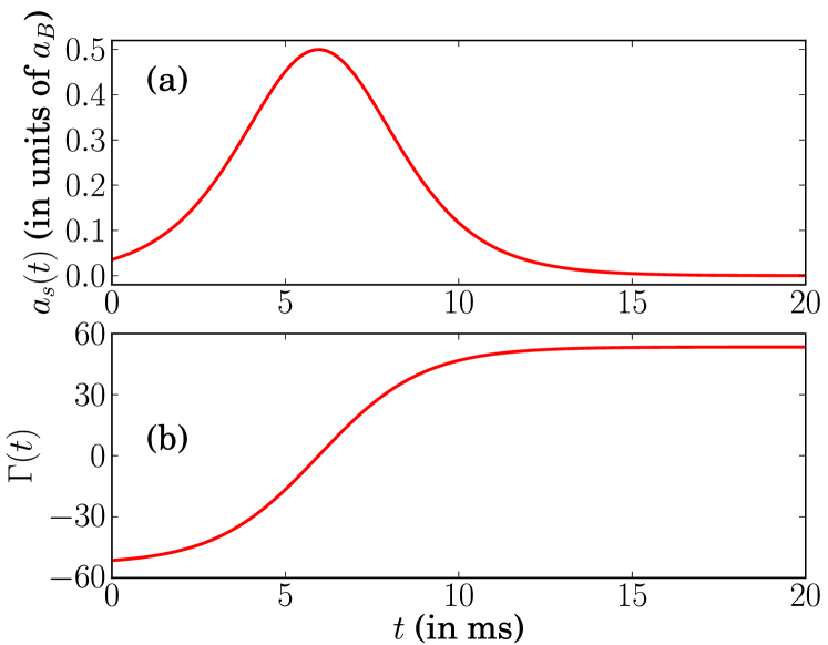
Figure 1: (color online) Choice of the atomic scattering length $a_{s}(t)$ and gain term $\Gamma(t)$ as a function of time for time-independent expulsive harmonic trap potential $V(x)=-\Omega_{0}^{2}x^{2}/2$, $\Omega_{0}=\text{constant}$.

Fig. 1 shows one such possible gain term $\Gamma(t)=\omega_{\perp}\Omega_{0}\tanh(\Omega_{0}t+\delta)$ and the atomic scattering length $a_{s}(t)=\frac{1}{2}a_{B}R(t)=\frac{1}{2}a_{B}\,\mbox{sech}^{2}(\Omega_{0}t+\delta)$, which can be experimentally realized by varying the external magnetic field as

$$B(t)=B_{0}+\frac{a_{s}^{0}\,\,\,\Delta}{a_{s}^{0}-\frac{1}{2}a_{B}\mbox{sech}^{2}(\Omega_{0}t+\delta)}.$$ (23)

One may note that such a form of scattering length $a_{s}(t)$ has been realized in ⁷Li and ⁸⁵Rb atoms Strecker et al. (2002); Khaykovich et al. (2002); Courteille et al. (1998). Similarly the gain term $\Gamma(t)$ can be experimentally realized by pumping of atoms optically as demonstrated in Refs. Davis et al. (2000); Köhl et al. (2002).

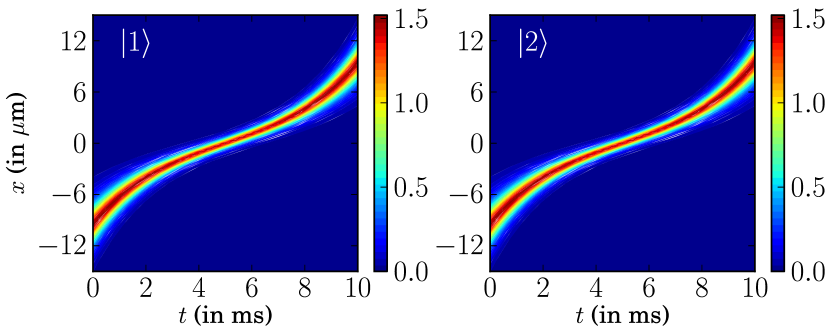
Figure 2: (color online) One-soliton solution for time-independent expulsive harmonic trap potential $V(x)=-\Omega_{0}^{2}x^{2}/2$ and $\gamma(t)=\Omega_{0}\tanh(\Omega_{0}t+\delta)$. The parameters are $k_{1}=1+0.5i$, $\alpha_{1}^{(1)}=\alpha_{1}^{(2)}=1.0$, $\Omega_{0}=890/53$ and $r_{0}=0.5$.

For $N=1$, we get the one-soliton solution of the coupled GP equation (1) from Eq. (22). As noted above, if we choose $\gamma(t)=\Omega_{0}\tanh(\Omega_{0}t+\delta)$, the intensity of the soliton is constant. Figure 2 shows the bright-bright one-soliton solution for the two components $|1\rangle=|\Psi_{1}|$ and $|2\rangle=|\Psi_{2}|$ for the above gain term where the amplitude of the wave packet remains constant. For the $N=2$ case we get the two-soliton solution of  (1) from Eq. (22). In this case, elastic collision occurs only for the specific choice of the parameters $(\alpha_{1}^{(1)}/\alpha_{2}^{(1)})=(\alpha_{1}^{(2)}/\alpha_{2}^{(2)})$, see Eqs. (20) and (22). For all other choices of the parameter values, shape changing/matter redistribution interaction occurs.

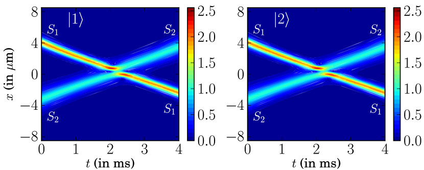
Figure 3: (color online) Elastic interaction of bright-bright two solitons for time-independent expulsive harmonic trap potential $V(x)=-\Omega_{0}^{2}x^{2}/2$ and $\gamma(t)=\Omega_{0}\tanh(\Omega_{0}t+\delta)$ for $\alpha_{1}^{(1)}=\alpha_{1}^{(2)}=\alpha_{2}^{(1)}=\alpha_{2}^{(2)}=1$. The parameters are $k_{1}=1+i$, $k_{2}=2-i$, $\Omega_{0}=0.06$ and $r_{0}=0.5$.

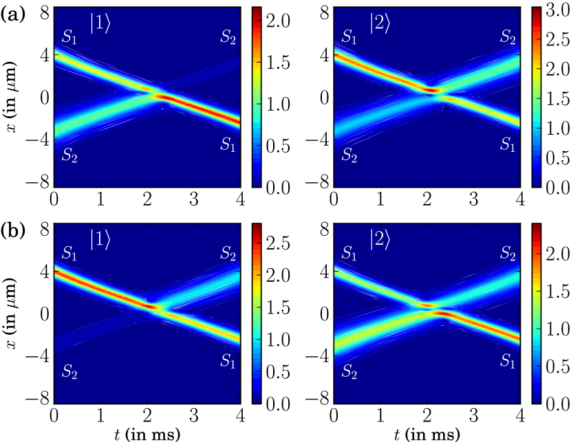
Figure 4: (color online) Shape changing interactions of bright-bright two solitons for time-independent expulsive harmonic trap potential $V(x)=-\Omega_{0}^{2}x^{2}/2$ and $\gamma(t)=\Omega_{0}\tanh(\Omega_{0}t+\delta)$ for (a): $\alpha_{1}^{(1)}=\alpha_{1}^{(2)}=\alpha_{2}^{(2)}=1$, $\alpha_{2}^{(1)}=(39+80i)/89$ and for (b): $\alpha_{1}^{(1)}=(0.02+0.1i)$, $\alpha_{2}^{(1)}=\alpha_{1}^{(2)}=\alpha_{2}^{(2)}=1$. The other parameters are $k_{1}=1+i$, $k_{2}=2-i$, $\Omega_{0}=0.06$ and $r_{0}=0.5$.

Fig. 3 shows the elastic interaction of the bright-bright two-soliton solution for $k_{1}=1+i$, $k_{2}=2-i$, $\alpha_{1}^{(1)}=\alpha_{1}^{(2)}=\alpha_{2}^{(1)}=\alpha_{2}^{(2)}=1$. Here the intensity of the two solitons ($S_{1}$ and $S_{2}$) in both the components are unchanged before and after interaction. The two distinct possibilities of the shape changing two-soliton interaction are shown in Figs. 4(a) and 4(b), see also Table 1(a). Figs. 4(a) illustrate the shape changing two-soliton interaction for $k_{1}=1+i$, $k_{2}=2-i$, $\alpha_{1}^{(1)}=\alpha_{1}^{(2)}=\alpha_{2}^{(2)}=1$, $\alpha_{2}^{(1)}=(39+80i)/89$. Here the intensity of the soliton $S_{1}$ gets enhanced

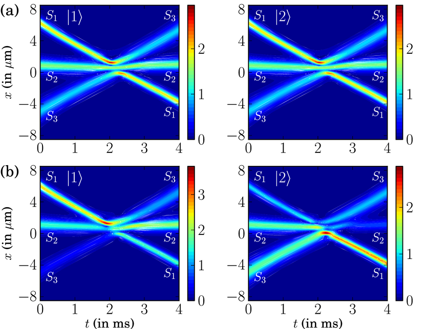
Figure 5: (color online) Bright-bright three soliton interactions: (a) Elastic interaction for $\alpha_{1}^{(1)}=\alpha_{1}^{(2)}=\alpha_{2}^{(1)}=\alpha_{2}^{(2)}=\alpha_{3}^{(1)}=\alpha_{3}^{(2)}=1$ and (b) Shape changing interaction for $\alpha_{1}^{(1)}=0.39+0.1i$, $\alpha_{2}^{(1)}=0.3+0.2i$, $\alpha_{3}^{(1)}=1.0$, $\alpha_{1}^{(2)}=(80.0-80i)/89.0$, $\alpha_{2}^{(2)}=0.6+0.2$, $\alpha_{3}^{(2)}=(89.0+80i)/89.0$ for time-independent expulsive harmonic trap potential $V(x)=-\Omega_{0}^{2}x^{2}/2$ and $\gamma(t)=\Omega_{0}\tanh(\Omega_{0}t+\delta)$. The other parameters are $k_{1}=1+0.5i$, $k_{2}=1.5$, $k_{3}=2-1.5i$, $\Omega_{0}=0.06$ and $r_{0}=0.5$.

while that of soliton $S_{2}$ is suppressed after interaction in the component $|1\rangle$, whereas in the component $|2\rangle$ it gets reversed. Fig. 4(b) shows another possible way of the shape changing two-soliton interaction for $k_{1}=1+i$, $k_{2}=2-i$, $\alpha_{1}^{(1)}=(0.02+0.1i)$, $\alpha_{2}^{(1)}=\alpha_{1}^{(2)}=\alpha_{2}^{(2)}=1$. Here in contrast to the above [cf. Figs. 4 (a)], the intensity of the soliton $S_{1}$ gets suppressed while that of soliton $S_{2}$ is enhanced after interaction in the component $|1\rangle$, whereas in the component $|2\rangle$ it gets reversed similar to the well studied case of Manakov system Radhakrishnan et al. (1997); Kanna and Lakshmanan (2001, 2003).

For the $N=3$ case, we get the three-soliton solutions of the coupled GP equation (1) from Eq. (22). Here elastic interaction occurs only for $\alpha_{1}^{(1)}:\alpha_{2}^{(1)}:\alpha_{3}^{(1)}=\alpha_{1}^{(2)}:\alpha_{2}^{(2)}:\alpha_{3}^{(2)}$ and for all other choice of parameters, matter redistribution interaction occurs. Fig. 5(a) shows the elastic interaction of bright-bright $3$-soliton ($N=3$ case) solution for $k_{1}=1+0.5i$, $k_{2}=1.5$, $k_{3}=2-1.5i$, $\alpha_{1}^{(1)}=\alpha_{1}^{(2)}=\alpha_{2}^{(1)}=\alpha_{2}^{(2)}=\alpha_{3}^{(1)}=\alpha_{3}^{(2)}=1$. Here the intensities of the three solitons in both the components are unchanged before and after interactions. Fig. 5(b) shows the shape changing interactions of bright-bright 3-soliton solution for $\alpha_{1}^{(1)}=0.39+0.1i$, $\alpha_{2}^{(1)}=0.3+0.2i$, $\alpha_{3}^{(1)}=1.0$, $\alpha_{1}^{(2)}=(80.0-80i)/89.0$, $\alpha_{2}^{(2)}=0.6+0.2$, $\alpha_{3}^{(2)}=(89.0+80i)/89.0$. Here the intensity of the soliton $S_{1}$ gets suppressed ($S$) while that of solitons $S_{2}$ and $S_{3}$ are enhanced ($E$) after interaction in the component $|1\rangle$, whereas in the component $|2\rangle$ it gets reversed. The six distinct possibilities of shape changing interactions of three soliton solutions are shown in Table 1(b).

Table 1: Possible combinations of matter redistributions of two solitons ($N=2$ case) and three solitons ($N=3$ case) under collision in component $|1\rangle$. $E$ stands for enhancement of intensity while $S$ represent suppression. See also Ref. Kanna and Lakshmanan (2001)

	(a) $N=2$ case
case	$S_{1}$	$S_{2}$
1	$E$	$S$
2	$S$	$E$
	(b) $N=3$ case
case	$S_{1}$	$S_{2}$	$S_{3}$
1	$E$	$S$	$S$
2	$S$	$E$	$S$
3	$S$	$S$	$E$
4	$S$	$E$	$E$
5	$E$	$S$	$E$
6	$E$	$E$	$S$

The above three soliton interaction process is equivalent to two pairwise interactions. Kanna and Lakshmanan  Kanna and Lakshmanan (2001, 2003) have shown that for the corresponding Manakov system the first interaction is controlled by the parameters $\alpha_{1}^{(1)}$, $\alpha_{2}^{(1)}$, $\alpha_{1}^{(2)}$, $\alpha_{2}^{(2)}$, $k_{1}$, $k_{2}$ and the second interaction is controlled by $\alpha_{3}^{(1)}$, $\alpha_{3}^{(2)}$ and $k_{3}$.

Fig. 6 depicts the shape restoring property of soliton $S_{1}$ during its interaction with the other two solitons, $S_{2}$ and $S_{3}$ for time-independent

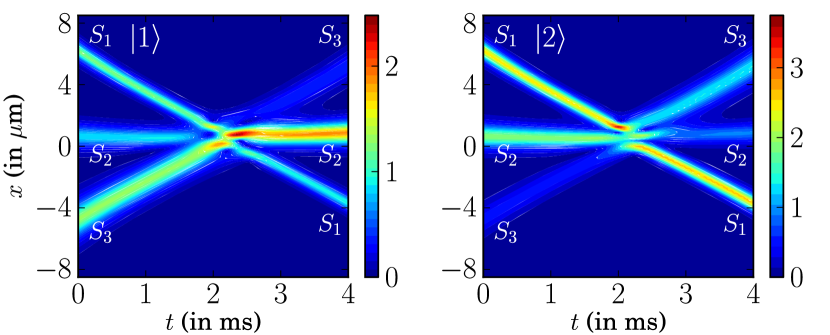
Figure 6: (color online) Shape restoring property of $S_{1}$ in three solitons interactions for time-independent expulsive harmonic trap potential $V(x)=-\Omega_{0}^{2}x^{2}/2$ and $\gamma(t)=\Omega_{0}\tanh(\Omega_{0}t+\delta)$ for the choice of the parameters $\alpha_{1}^{(1)}=(39-80i)/89$, $\alpha_{2}^{(1)}=(39+80i)/89$, $\alpha_{3}^{(1)}=0.3+0.2i$, $\alpha_{1}^{(2)}=0.39$, $\alpha_{2}^{(2)}=\alpha_{3}^{(2)}=1$, $k_{1}=1+1.5i$, $k_{2}=1.5$, $k_{3}=2-1.5i$, $\Omega_{0}=0.06$ and $r_{0}=0.5$.

expulsive harmonic trap potential $V(x)=-\Omega_{0}^{2}x^{2}/2$ for the choice of the parameters $\alpha_{1}^{(1)}=(39-80i)/89$, $\alpha_{2}^{(1)}=(39+80i)/89$, $\alpha_{3}^{(1)}=0.3+0.2i$, $\alpha_{1}^{(2)}=0.39$, $\alpha_{2}^{(2)}=\alpha_{3}^{(2)}=1$, $k_{1}=1+1.5i$, $k_{2}=1.5$, $k_{3}=2-1.5i$. Here the intensity of the soliton $S_{1}$ is unchanged after its interactions with the other two solitons $S_{2}$ and $S_{3}$ in both the components, while the intensities of solitons $S_{2}$ and $S_{3}$ get changed. The condition for the choice of the parameters for the shape restoration of soliton $S_{1}$ is given in Ref. Kanna and Lakshmanan (2003). Note that the shape restoring property is essential for the construction of universal logic gates which are necessary for computing Steiglitz (2000); Kanna and Lakshmanan (2003). The above type of elastic, shape changing interactions and shape restoring property of solitons during the interactions are similar to the study of Kanna and Lakshmanan Kanna and Lakshmanan (2001, 2003) in the context of optical computing, where the intensities of light pulses are transformable between two modes. Here, the shape changing interactions are interpreted as the transform of the fraction of atoms between the two components, which can be achieved experimentally by suitable tuning of atomic scattering length and gain/loss term. Note that exact analytical representations for the soliton switching can be given in the form of linear fractional tranformations leading to logic gates as in the case of optical systems, see Ref. Steiglitz (2000); Kanna and Lakshmanan (2003). This type of shape changing soliton interactions can be used (as disscussed in Refs. Folman et al. (2000); Folman and Schmiedmayer (2001); Petrov et al. (2009)) in the matter wave switching devices, logic gates and quantum information processing as in the case of optical computing.

IV.2 Periodically Modulated Trap Potential

Next, if we choose the periodically varying atomic scattering length Baizakov et al. (2005) $R(t)=1+\omega\cos(\omega t+\delta)$ and the corresponding gain term

$$\gamma(t)=\displaystyle\frac{\omega^{2}\sin(\omega t+\delta)}{2\left[1+\omega\cos(\omega t+\delta)\right]},\;\;\;\omega\leq 1,$$ (24)

with $\delta$ as a constant, we get $\tilde{R}(t)=\sqrt{1+\omega\cos(\omega t+\delta)}$ from Eq. (5)and the periodically modulated trap frequency from the integrability condition (13) as

$$\Omega^{2}(t)=\omega^{2}\left\{1-\frac{4+10\omega\cos\tilde{\theta}+3\omega^{2}\left[1+\cos^{2}\tilde{\theta}\right]}{4\left[1+\omega\cos\tilde{\theta}\right]^{2}}\right\},$$ (25)

where $\tilde{\theta}=\omega t+\delta$. The intensity of soliton also remains constant for this case but the width of the soliton is periodically varying with time (that is, inversely proportional to $\sqrt{\tilde{R}(t)}$). Fig. 7 shows the gain term

$$\Gamma(t)=\displaystyle\frac{\omega_{\perp}\omega^{2}\sin(\omega t+\delta)}{2[1+\omega\cos(\omega t+\delta)]},$$ (26)

which can can also be experimentally realized by suitable optical pumping, and the corresponding choice of atomic scattering length $a_{s}(t)=\frac{a_{B}}{2}\left[1+\omega\cos(\omega t+\delta)\right]$

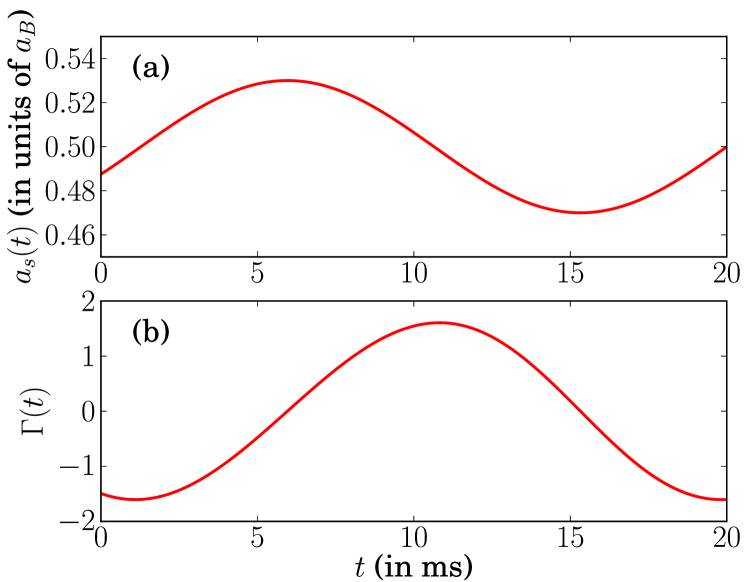
Figure 7: (color online) Form of the (a) atomic scattering length $a_{s}(t)$ and (b) gain or loss term $\Gamma(t)$ as a function of time for the periodically modulated harmonic potential with the trap frequency (25).

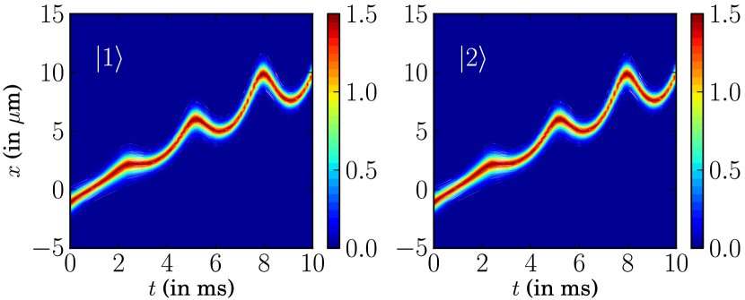
Figure 8: (color online) One-soliton solution for the periodically modulated harmonic potential with trap frequency (25). The parameters are fixed as $k_{1}=1+0.5i$, $\alpha_{1}^{(1)}=\alpha_{1}^{(2)}=1.0$, $\omega=0.4$ and $r_{0}=0.5$.

which may be experimentally realized by periodically tuning the external magnetic field as

$$B(t)=B_{0}+\frac{a_{s}^{0}\,\,\,\Delta}{a_{s}^{0}-\frac{1}{2}a_{B}\left[1+\omega\cos(\omega t+\delta)\right]}.$$ (27)

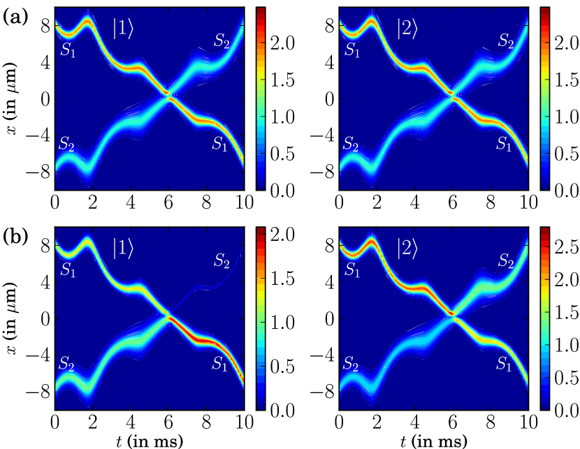
Figure 9: (color online) Bright-bright two soliton interactions for the periodically modulated harmonic potential. (a) Elastic collision for $\alpha_{1}^{(1)}=\alpha_{1}^{(2)}=\alpha_{2}^{(1)}=\alpha_{2}^{(2)}=1$ and (b) Shape changing collision for $\alpha_{1}^{(1)}=\alpha_{1}^{(2)}=\alpha_{2}^{(2)}=1$, $\alpha_{2}^{(1)}=(39+80i)/89$. The other parameters are fixed as $k_{1}=1+i$, $k_{2}=2-i$, $\omega=0.4$ and $r_{0}=0.5$.

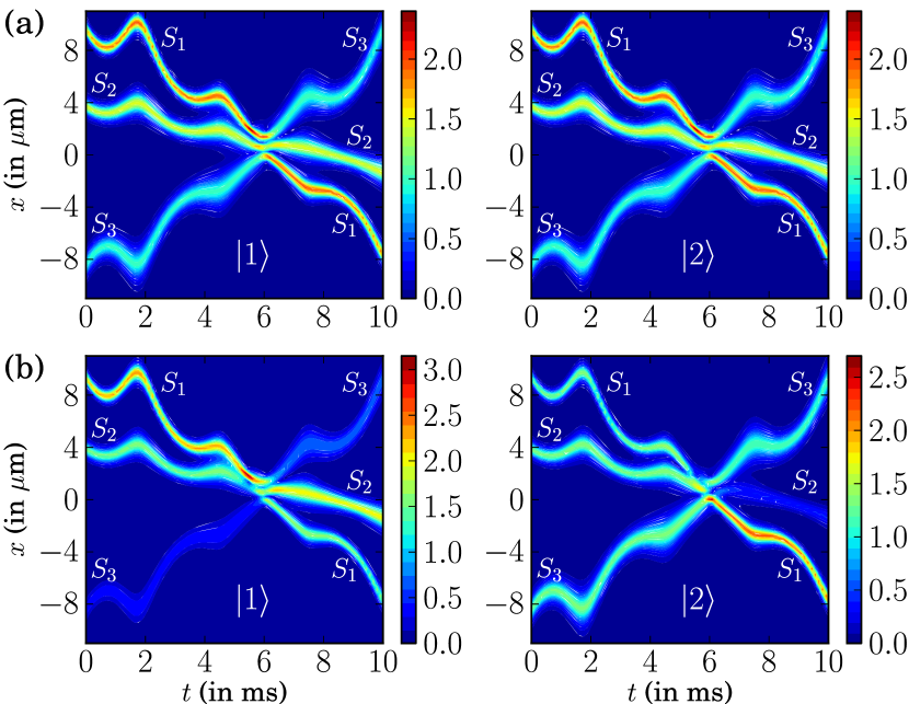
Figure 10: (color online) Bright-bright three soliton interactions for the periodically modulated harmonic trap potential. (a) Elastic collision for $\alpha_{1}^{(1)}=\alpha_{1}^{(2)}=\alpha_{2}^{(1)}=\alpha_{2}^{(2)}=\alpha_{3}^{(1)}=\alpha_{3}^{(2)}=1$ and (b) Shape changing collision for $\alpha_{1}^{(1)}=0.39+0.1i$, $\alpha_{2}^{(1)}=0.3+0.2i$, $\alpha_{3}^{(1)}=1.0$, $\alpha_{1}^{(2)}=(80.0-80i)/89.0$, $\alpha_{2}^{(2)}=0.6+0.2$, $\alpha_{3}^{(2)}=(89.0+80i)/89.0$. The parameters are $k_{1}=1+i$, $k_{2}=1.5-0.5i$, $k_{3}=2-i$, $\omega=0.4$ and $r_{0}=0.5$.

Fig. 8 shows the snake-like effect of the one-soliton solution for the above periodically modulated trap potential with $R(t)=\left[1+\omega\cos(\omega t+\delta)\right]$ and $\gamma(t)$ as given in Eq. (24), where the intensity of the soliton remains constant in both the components while the width of the soliton varies periodically with time. Note that the oscillation of the soliton goes on increasing with time due to the fact that the width of the soliton is inversely proportional to $\tilde{R}(t)$. It is of importance to note that recently, in scalar nonautonomous NLS equation for BEC Rajendran et al. (2010) and optical solitons Serkin and Hasegawa (2000), a similar kind of snake-like effect has been demonstrated.

Next we analyze different types of two soliton interactions for the periodically modulated potential for suitable choice of other parameters. Fig. 9(a) shows the elastic collision of snake like bright-bright two solitons while Fig. 9(b) shows shape changing collision of snake-like bright-bright two solitons for $\omega=0.4$. Figs. 10(a) and (b) depict the elastic collision and shape changing collision of snake-like bright-bright three-soliton solutions, respectively, for this case. The other parameters are the same as in the time independent expulsive harmonic potential case. The collision effects are similar to the ones discussed in the case of expulsive trap potential earlier but now the widths of solitons oscillate periodically with time because of the periodically varying atomic scattering length.

IV.3 Kink-like Modulated Trap Potential

Finally, if we choose $R(t)=1+\tanh(\omega t+\delta)$ and

$$\gamma(t)=\displaystyle-\frac{\omega}{4}\left[1-\tanh(\omega t+\delta)\right],$$ (28)

we get $\tilde{R}(t)=\sqrt{1+\tanh(\omega t+\delta)}$ and the integrability condition (13) gives

$$\Omega^{2}(t)=-\omega^{2}\left[1-\frac{\mbox{e}^{4\omega t}}{(1+\mbox{e}^{2\omega t})^{2}}\right],$$ (29)

which is a kink-like modulated trap.

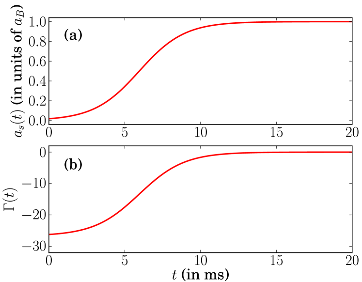
Figure 11: (color online) Choice of the (a) atomic scattering length $a_{s}(t)$ and (b) gain term $\Gamma(t)$ as a function of time for the kink-like modulated harmonic potential $V(x,t)=\displaystyle-\omega^{2}\left(1-\frac{\mbox{e}^{4\omega t}}{(1+\mbox{e}^{2\omega t})^{2}}\right)x^{2}$.

For the above case, we sketch the gain

$$\Gamma(t)=\displaystyle-\frac{\omega_{\perp}\omega}{4}\left[1-\tanh(\omega t+\delta)\right],$$ (30)

and the corresponding

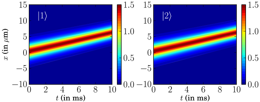
Figure 12: (color online) One-soliton solution for the kink-like trap potential. The parameters are $k_{1}=1+0.5i$, $\alpha_{1}^{(1)}=\alpha_{1}^{(2)}=1.0$, $\omega=0.06$ and $r_{0}=0.75$.

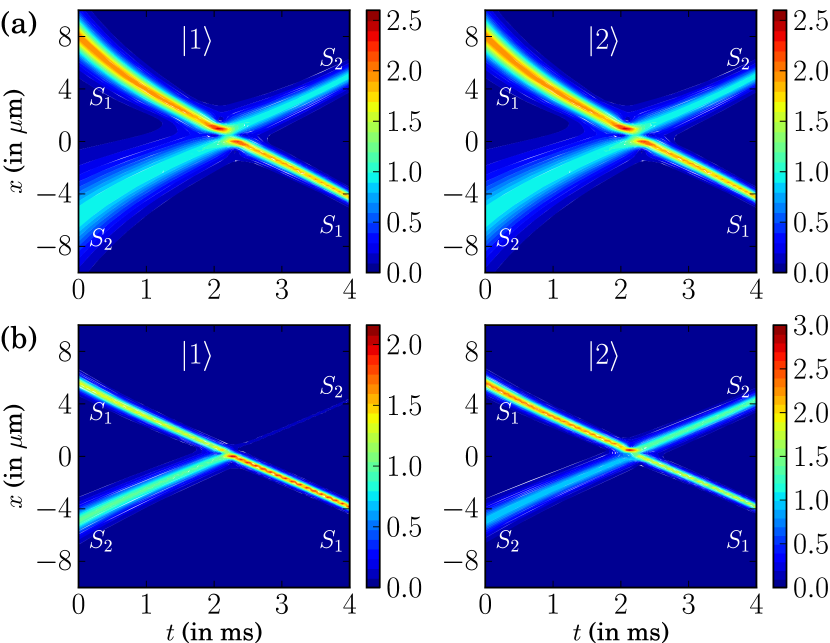
Figure 13: (color online) Bright-bright two soliton interactions for the kink-like modulated harmonic trap potential. (a) Intensity unchanged under the collision for $\alpha_{1}^{(1)}=\alpha_{1}^{(2)}=\alpha_{2}^{(1)}=\alpha_{2}^{(2)}=1$. (b) Matter redistribution collision for $\alpha_{1}^{(1)}=\alpha_{1}^{(2)}=\alpha_{2}^{(2)}=1$, $\alpha_{2}^{(1)}=(39+80i)/89$. The parameters are $k_{1}=1+i$, $k_{2}=2-i$, $\omega=0.06$ and $r_{0}=0.4$

choice of atomic scattering length $a_{s}(t)=\frac{a_{B}}{2}\left[1+\tanh(\omega t+\delta)\right]$ in Fig. 11. The form (30) of the gain can again be experimentally realized by continuously loading the external atoms into the condensate by optical pumping as in the case of Refs. Davis et al. (2000); Köhl et al. (2002) and the atomic scattering length can be realized by a kink-like tuning of the external magnetic field as

$$B(t)=B_{0}+\frac{a_{s}^{0}\,\,\,\Delta}{a_{s}^{0}-\frac{1}{2}a_{B}\left[1+\tanh(\omega t+\delta)\right]}.$$ (31)

Fig. 12 shows the one-soliton solution for the kink-like modulated trap potential with $R(t)=1+\tanh(\omega t+\delta)$ and

$$\gamma(t)=\displaystyle-\frac{\omega}{4}\left[1-\tanh(\omega t+\delta)\right].$$

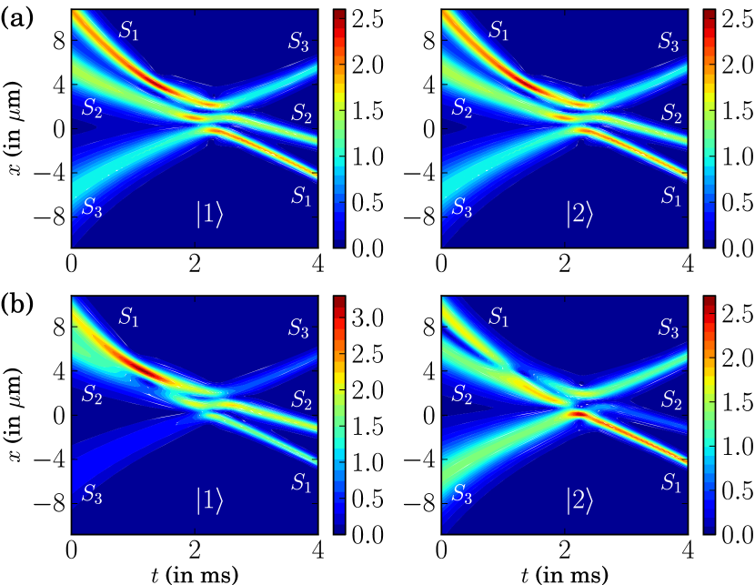
Figure 14: (color online) Bright-bright three soliton interactions for the kink-like modulated harmonic trap potential. (a) Intensity unchanged collision for $\alpha_{1}^{(1)}=\alpha_{1}^{(2)}=\alpha_{2}^{(1)}=\alpha_{2}^{(2)}=\alpha_{3}^{(1)}=\alpha_{3}^{(2)}=1$. (b) Matter redistribution collision for $\alpha_{1}^{(1)}=0.39+0.1i$, $\alpha_{2}^{(1)}=0.3+0.2i$, $\alpha_{3}^{(1)}=1.0$, $\alpha_{1}^{(2)}=(80.0-80i)/89.0$, $\alpha_{2}^{(2)}=0.6+0.2$, $\alpha_{3}^{(2)}=(89.0+80i)/89.0$. The parameters are $k_{1}=1+i$,$k_{2}=1.5-0.5i$, $k_{3}=2-i$, $\omega=0.06$ and $r_{0}=0.4$

Here the intensity of solitons in both the components are constant while the width is decreasing with time (that is inversely proportional to $\sqrt{\tilde{R}(t)}$).

Next we analyze the two-soliton ($N=2$) and three-soliton ($N=3$) solutions for the two-component BECs with kink-like modulated harmonic trap potential. Fig. 13(a) shows the bright-bright intensity unchanged collision of two solitons while Fig. 13(b) shows matter redistribution collision of two solitons. The intensity unchanged and matter redistribution collisions of three-soliton solutions for the kink-like modulated potential are shown in Figs. 14(a) and 14(b), respectively. The other parameters are the same as in the time-independent potential case. Note that, here, the widths of the two and three solitons are also decreasing with time.

V Summary and conclusion

In summary, we have investigated the exact bright-bright multi-soliton solutions of the two-component BECs with time varying parameters such as trap frequency, s-wave scattering length and gain/loss term. On mapping the two coupled GP equations onto the coupled NLS equations under certain conditions, we have deduced different kinds of bright-bright one-soliton solutions and interaction of two solitons for time independent expulsive harmonic trapping potential, periodically modulated trap potential and kink-like modulated potential. We have shown the shape changing and elastic interactions of bright-bright two-soliton and three-soliton solutions of the two component BECs. The present study provides an understanding of the possible mechanism for the fraction of atoms transform between the two components. Especially the shape changing collisions of matter wave solitons can used for matter wave switching devices, logic gates and quantum information processing. These elastic and shape changing interactions can be realized in experiments by suitable control of time dependent trap parameters, atomic interaction and interaction with thermal cloud.