EIT-based Vector Magnetometry in Linearly Polarized Light

Abstract

We develop a generalized principle of EIT vector magnetometry based on high-contrast EIT-resonances and the symmetry of atom-light interaction in the linearly polarized bichromatic fields. Operation of such vector magnetometer on the $D_{1}$ line of ⁸⁷Rb has been demonstrated. The proposed compass-magnetometer has an increased immunity to shifts produced by quadratic Zeeman and ac-Stark effects, as well as by atom-buffer gas and atom-atom collisions. In our proof-of-principle experiment the detected angular sensitivity to magnetic field orientation is $10^{-3}$deg$/$Hz^1/2, which is limited by laser intensity fluctuations, light polarization quality, and magnitude of the magnetic field.

I Introduction

The pure quantum state is a basic concept of quantum physics, which plays a key role in various applications, such as magnetometry, frequency standards, laser cooling, quantum information science, nonlinear optics, and ‘‘slow’’ and ‘‘fast’’ light experiments. The effect of electromagnetically induced transparency (EIT) Alzetta ; Arimondo ; Harris ; Fleisch has been successfully employed in all these applications.

The idea of EIT scalar magnetometer has been suggested in Scully . The steep dispersion of EIT media promises a dramatic improvement of the scalar magnetometer sensitivity. Since then different schemes for EIT magnetometry have been considered. Among them are schemes based on the nonlinear Faraday effect in a manifold of a single ground state Budker2 ; Novikova ; Stahler and a scheme in which the frequency shift of Zeeman sublevels of both ground states is detected Wynands . The sensitivity of EIT magnetometers is in the same range as magnetometers using optical pumping BudBud ; Bud . The recent modification of optically pumped magnetometers with suppressed spin-exchange broadening (so-called SERF-magnetometer) drastically improves sensitivity by a factor of $10^{3}$. It overcomes the sensitivity of SQUID magnetometers ($10^{-15}$ T$/$Hz^1/2) Romalis . Unfortunately, SERF-magnetometers work in small fields that are less than 0.1 $\mu$T, which is significantly weaker than geomagnetic field.

For many applications it is preferable to know not only the scalar – but also the direction of the magnetic field. To achieve this, individual coils are installed for each of the $X$, $Y$, and $Z$ axes in a scalar magnetometer. The coils are used to induce small modulations of the magnetic field along each axes, which gives the information about $B_{x}$ and $B_{y}$ field components Fairweather ; Gravrand ; Alexandrov2 . This allows the orientation of the vector B to be reconstructed. The first schemes of EIT vector magnetometer have been proposed in Wynands2 ; Lee . However, the angular accuracy of these magnetometers strongly depends on mathematical models (describing the atom-field interaction and light field propagation) used to extract the magnetic field direction from experimental signals. The reviews of existing all-optical magnetometers were published in Romalis2 ; Alexandrov .

In the present paper we show that employing the unique features of high-contrast EIT resonances on the $D_{1}$ line of ⁸⁷Rb allows us to find new approaches to the atomic vector magnetometery and to model a relevant device in which the scalar and vector properties of magnetic field can be measured separately or simultaneously. Our approach does not require the mathematical models to reconstruct a three-dimensional orientation of the magnetic field.

II General description of the problem

EIT phenomenon is closely connected to the so-called coherent population trapping (CPT) Alzetta ; Arimondo in which the atom-field interaction $-(\widehat{\bf d}{\bf E})$ of the pure quantum state $|dark\rangle$ is zero:

$$-(\widehat{\bf d}{{\bf E}})|dark\rangle=0\,.$$ (1)

This state is a special coherent superposition of the ground state Zeeman sublevels that neither absorbs nor emits light. Dark states lead to the highest contrast of EIT resonances. Thus, the preparation of pure states is crucial for any of the above mentioned applications.

The generalized problem of the production of pure quantum states by bichromatic elliptically polarized field was solved in Y . In icono05 ; lin||lin JETP ; Serezha it was theoretically and experimentally demonstrated that the $D_{1}$ line of ⁸⁷Rb has unique level structure for the production of pure dark states using bichromatic linearly polarized light (so-called lin$||$lin field), where the resonant interaction occurs via the upper energy level $F_{e}$=1. There are two pairs of dark states, where each dark state corresponds to the separate $\Lambda$-scheme (see Fig. 1). One pair corresponds to $\Lambda_{1}$ and $\Lambda_{2}$ schemes in Fig. 1a and involves the following two-photon transitions: $|F_{1}=1,m=-1\rangle\leftrightarrow|F_{2}=2,m=+1\rangle$ and $|F_{1}=1,m=+1\rangle\leftrightarrow|F_{2}=2,m=-1\rangle$. In our experiments the EIT resonances of these pairs have a high contrast (50%) and transmission (60%) (solid line in Fig. 2). Both $\Lambda_{1}$ and $\Lambda_{2}$ transitions contribute to EIT resonance (the dependence of transmission on the difference of the two optical frequencies) that is attractive for applications in chip-size atomic clocks (CSAC) since it provides high contrast and smaller (by factor 1.33) quadratic dependence on the magnetic field compared to the regular atomic clock transition $|F_{1}=1,m=0\rangle\leftrightarrow|F_{2}=2,m=0\rangle$ Evelina ; Novikova2 ; Mikhailov2 . Note that the shifts of zero magnetic sublevels and the frequency of 0-0 transition do not depend linearly on magnetic field, while sublevels with $m=\pm 1$ do. The electron $g$-factors of the ground states $F_{1,2}$ have the same magnitude but opposite sings (see Fig. 1). As a result, the residual linear shifts (due to a nuclear contribution) of the $\Lambda_{1}$ and $\Lambda_{2}$ transitions are 250 times smaller than the shifts of individual magnetic sublevels $m=\pm 1$ ($\approx\pm$28 Hz$/$$\mu$T instead of $\approx\pm$7 kHz$/$$\mu$T). However, these residual shifts are manifested only in a small broadening of the resonance lineshape, while the center of the resulting $\Lambda_{1,2}$-resonance has a zero linear sensitivity to the magnetic field (due to the symmetry of $\Lambda_{1}$ and $\Lambda_{2}$ systems for the lin$||$lin light) icono05 ; lin||lin JETP .

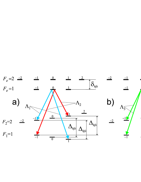
Figure 1: Pure $\Lambda$-systems at the $D_{1}$ line of ⁸⁷Rb: non-sensitive (a) and sensitive (b) to magnetic field. Here we do not show Zeeman shifts for upper hyperfine levels with $F_{e}$=1,2.

The other pair of $\Lambda$-schemes ($\Lambda_{3}$ and $\Lambda_{4}$ in Fig. 1b) gives the two-photon transitions: $|F_{2}=2;m=-1\rangle\leftrightarrow|F_{1}=1;m=-1\rangle$ and $|F_{2}=2;m=+1\rangle\leftrightarrow|F_{1}=1;m=+1\rangle$ that strongly depend on magnetic field and can be used for measurment of the magnetic field magnitude, as it was noted in lin||lin JETP .

To produce quantum dark states (1) for the $D_{1}$ line of ⁸⁷Rb, we use (in conformity with icono05 ; lin||lin JETP ) a linearly polarized bichromatic running wave ${\bf E}({\bf r},t)$ with close frequencies $\omega_{1}$ and $\omega_{2}$ and wavevector $\mathbf{k}$ (i.e. lin$||$lin configuration):

$${\bf E}({\bf r},t)=(E_{1}e^{-i\omega_{1}t}+E_{2}e^{-i\omega_{2}t})e^{i{\bf kr}}{\bf e}+c.c.\,,$$ (2)

where ${\bf e}$ is a unit vector of the linear polarization, and $E_{1,2}$ are the scalar amplitudes of the corresponding frequency components. The interaction occurs in the presence of the static magnetic field ${\bf B}$. If the $z$-axis is directed along the vector ${\bf B}$, the vector ${\bf e}$ can be expressed in a spherical basis {${\bf e}_{0}$=${\bf e}_{z}$, ${\bf e}_{\pm 1}$$=$$\mp$$({\bf e}_{x}$$\pm$$i{\bf e}_{y})$/$\sqrt{2}$}:

$${\bf e} = \sum_{q=0,\pm 1}e^{(q)}{\bf e}_{q}=\cos{\theta}\,{\bf e}_{0}-\frac{\sin{\theta}}{\sqrt{2}}(\bf{e}_{+1}-\bf{e}_{-1})\,,$$ (3)

where $\theta$ is the angle between vectors ${\bf B}$ and ${\bf e}$; $e^{(q)}$ are the contravariant components of the vector ${\bf e}$. Note that for linear polarization its circular components ($\sigma_{\pm}$) are always equal:

$$|e^{(+1)}|=|e^{(-1)}|=|\sin{\theta}|/\sqrt{2}\,.$$ (4)

As it will be shown below, the symmetry (4) is one of principal points of EIT magnetometry in a linear polarized field.

In the resonant approximation we assume that the frequency component $\omega_{j}$ ($j$=1,2) excites atoms only from the hyper-fine ground level $F_{j}$ (Fig. 1). From here on, we use the interaction representation

$$e^{-i{\cal E}_{Fm}t/\hbar}|F,m\rangle\to|F,m\rangle\,,$$

where ${\cal E}_{Fm}$ is the energy of the level $|F,m\rangle$ in which the Zeeman shift is included. The operator of an atom-field interaction $-(\widehat{\bf d}{\bf E})=\widehat{V}+\widehat{V}^{\dagger}$ under the resonant approximation takes the form:

$$\widehat{V} = e^{i{\bf kr}}\sum_{q=0,\pm 1}e^{(q)}\times$$

$${}\biggl{[}E_{1}\sum_{F_{e},\mu,m_{1}}d_{F_{e}F_{1}}e^{-i\delta^{(1)}_{\mu m_{1}}t}C^{F_{e}\mu}_{F_{1}m_{1},1q}|F_{e},\mu\rangle\langle F_{1},m_{1}|+$$

$$E_{2}\sum_{F_{e},\mu,m_{2}}d_{F_{e}F_{2}}e^{-i\delta^{(2)}_{\mu m_{2}}t}C^{F_{e}\mu}_{F_{2}m_{2},1q}|F_{e},\mu\rangle\langle F_{2},m_{2}|\biggr{]}.$$

Here $d_{F_{e}F_{1}}$ and $d_{F_{e}F_{2}}$ denote reduced matrix elements of corresponding optical transitions $F_{1}\to F_{e}$ and $F_{2}\to F_{e}$, $C^{F_{e}m_{e}}_{F_{j}m_{j},1q}$ are Clebsch-Gordan coefficients, and $\delta^{(j)}_{\mu m_{j}}=\omega_{j}-({\cal E}_{F_{e}\mu}-{\cal E}_{F_{j}m_{j}})/\hbar$ for $j=1,2$ are corresponding one-photon detunings.

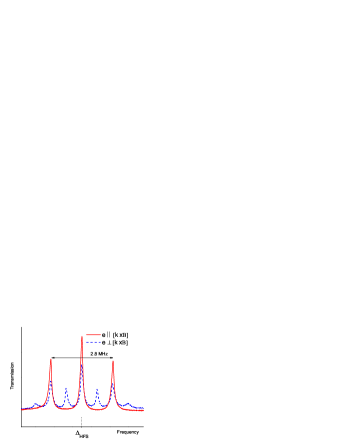
Figure 2: EIT resonance transmission:
(solid line) – the case $\mathbf{e}$$\parallel$$\mathbf{n}$. The central resonance corresponds to the $\Lambda_{1}$ and $\Lambda_{2}$ schemes (Fig. 1a). This resonance has 120 kHz width and $\sim 60$$\%$ transmission.
(dashed line) – the case $\mathbf{e}$$\perp$$\mathbf{n}$. Magnetic field has magnitude 1 G, the angle between $\mathbf{B}$ and $\mathbf{k}$ equals 20^∘.

For alkaline atoms with nuclear spin $I_{n}$ we have $F_{1}$$=$$(I_{n}$$-$$1/2)$ and $F_{2}$$=$$(I_{n}$$+$$1/2)$. The corresponding electron ground-state Land$\acute{\mbox{e}}$ factors have the same absolute value but opposite signs: $g$=$-g_{F_{1}}$=$g_{F_{2}}$=($I_{n}$$+$$1/2)^{-1}$ (for ⁸⁷Rb $g$=$1/2$). Then in the linear approximation of the dependence on the magnetic field ${\bf B}$ and neglecting the nuclear magneton contribution it is easy to count the number of splitted two-photon resonances. For arbitrary directed ${\bf B}$ there are (4$I_{n}+$1) two-photon resonances in transmissions versus Raman detuning $\delta_{R}$=($\omega_{1}$$-$$\omega_{2}$$-$$\Delta_{hfs}$) dependencies centered at the points $\delta_{R}$=$l$$g$$\mu_{B}$$|{\bf B}|$/$\hbar$ ($l$=$-2I_{n}$,…,$2I_{n}$), where $\mu_{B}$ is Bohr magneton. For example, in ⁸⁷Rb ($I_{n}$=3/2) we have seven two-photon resonances (the blue dashed line in Fig. 2). In the particular case of $\mathbf{B}$$\perp$$\mathbf{e}$, the number of two-photon resonances equals to $2I_{n}=3$ (the red solid line in Fig. 2).

III EIT-based 3D compass

First we examine in detail the central resonance (near $\delta_{R}$=0). It will be shown below that this resonance can be used for the vector magnetometer due to the strong dependence of transmission on the mutual orientation of vectors ${\bf e}$ and ${\bf B}$ (i.e. on the angle $\theta$ in Eq.(3)). The following two transitions take place in formation of the central two-photon resonance: $|F_{1}$,m=$-1\rangle$$\leftrightarrow$$|F_{2}$,m=$+1\rangle$ and $|F_{1}$,m=$+1\rangle$$\leftrightarrow$$|F_{2}$,m=$-1\rangle$, for which the energy difference equals $\hbar$$\Delta_{hfs}$ (Fig. 1a). The third two-photon transition $|F_{1}$,m=$0\rangle$$\leftrightarrow$$|F_{2}$,m=$0\rangle$ (between magnetically insensitive sublevels) is strongly suppressed due to further destructive interference of contributions from the opposite circular components $\sigma_{\pm}$.

In the case of a resolved upper hyper-fine structure ($F_{e}$=1,2 in the Fig. 1), the two-photon resonance can be excited via separate level. Further we assume that the frequency components (2) are at the resonance with a single hyper-fine level $F_{e}$=1 (Fig. 1). Now let us consider a special case where the vectors ${\bf e}$ and ${\bf B}$ are mutually orthogonal ($\theta$=$\,\pi/2$), and, therefore, only two equal circular components ${\bf e}=-({\bf e}_{+1}-{\bf e}_{-1})/\sqrt{2}$ occur in the decomposition (3). It is seen from Fig. 1a that there is a two-photon resonance formed via pure $\Lambda_{1}$-scheme with Zeeman sublevels $|F_{1}$=1,m=$+1\rangle$ and $|F_{2}$=2,m=$-1\rangle$. Similarly, the $\Lambda_{2}$-scheme is realized with the other sublevel pairs $|F_{1}$=1,m=$-1\rangle$ and $|F_{2}$=2,m=$+1\rangle$. Both of these $\Lambda_{1,2}$-schemes are formed via the same common upper sublevel $|F_{e}$=1,m=$0\rangle$. As was mentioned before, the frequencies of these two-photon resonances are equal (neglecting the nuclear magneton contribution) to the frequency of the (0-0) resonance between sublevels $|F_{1}$=1,m=$0\rangle$ and $|F_{2}$=2,m=$0\rangle$.

The uniqueness of the situation arises from the overlapping the two ($|dark\rangle_{\Lambda_{1}}$ and $|dark\rangle_{\Lambda_{2}}$) dark states, which occur at the two-photon resonance, $\delta_{R}=0$. These states satisfy the equation (1) and have the following forms:

$$|dark\rangle_{\Lambda_{1,2}}=\frac{\sqrt{3}E_{2}|F_{1},m=\pm 1\rangle\mp E_{1}|F_{2},m=\mp 1\rangle}{\sqrt{|E_{1}|^{2}+3|E_{2}|^{2}}}.$$ (6)

The presence of such dark states in the ${\bf e}$$\perp$${\bf B}$ case leads to a high contrast of the central dark resonance near $(\omega_{1}-\omega_{2})$=$\Delta_{hfs}$ (i.e. $\delta_{R}$$\approx$$\,0$). This fact was predicted and experimentally demonstrated in icono05 ; lin||lin JETP .

In the general case of $\theta$$\neq$$\pi/2$ (that is $\cos(\theta)$$\neq$0) there are no pure $\Lambda$-schemes due to the $\pi$-polarized (along ${\bf B}$) component in decomposition (3). It leads to a smaller amplitude and contrast of the central two-photon $\Lambda_{1,2}$-resonance in comparison to the case of $\theta$=$\pi/2$. This fact will be used as a basis for determination of the magnetic field orientation (i.e. compass) in our approach.

The basic idea of our method can be explained in the following way. Assume that the wavevector ${\bf k}$ and the vector ${\bf B}$ have an arbitrary mutual orientation. We will use the amplitude of the central resonance (absorption, transmission or fluorescence) as the measured quantity (Fig. 2). There are two cases, where e and B are orthogonal to each other. More precisely, these situations arise if ${\bf e}$$||$${\bf n}$, where ${\bf n}$=$[{\bf k}\times{\bf B}]$ (Fig. 3). These cases correspond to the dark states (6), which lead to the maximal amplitude and contrast of the central resonance (as explained above).

Consider the dependence of the dark resonance amplitude, which is obtained by rotating the polarization vector ${\bf e}$ around fixed wavevector ${\bf k}$. This dependence can be presented as a function $A_{\bf k}$($\varphi$), where $\varphi$ is the angle between the vectors ${\bf e}$ and ${\bf n}$ (Fig. 3). Even the qualitative analysis, provided above, leads to the conclusion that the function $A_{\bf k}$($\varphi$) reaches its maximum at $\varphi$=0,$\,\pi$, i.e. when ${\bf e}$$\perp$${\bf B}$.

The essence of the measuring procedure could be represented by the following algorithm. At first, for a chosen vector ${\bf k}$=${\bf k}_{1}$, we get the $A_{{\bf k}_{1}}$($\varphi$) dependence by rotating the polarization vector ${\bf e}$ around wavevector ${\bf k}_{1}$. The maximum of this dependence corresponds to the direction of the vector ${\bf n}$=$[{\bf k}_{1}\times{\bf B}]$, which gives us the equation for the plane (${\bf k}_{1},{\bf B}$) formed by the vectors ${\bf k}_{1}$ and ${\bf B}$. Repeating the same procedure for another orientation of the wavevector ${\bf k}$=${\bf k}_{2}$ (for example, ${\bf k}_{2}$$\perp$${\bf k}_{1}$) provides the equation for the plane (${\bf k}_{2},{\bf B}$). The intersection line of the two planes (${\bf k}_{1},{\bf B}$) and (${\bf k}_{2},{\bf B}$) gives the 3D orientation of the vector ${\bf B}$ with an uncertainty of the sign.

The basic principle of our method is quite universal and does not depend on different experimental parameters (such as the $|E_{1}/E_{2}|$ ratio, one-photon detuning, relaxation constants, atom-atom collisions, nuclear magnetic momentum, and so on). This can be seen from the general symmetry of the problem. Indeed, suppose we have an arbitrary polychromatic wave propagating along a direction ${\bf k}$ and having the same linear polarization ${\bf e}$ for all frequency components. Also we assume that the atomic medium is isotropic in the absence of the light field. We determine the signal $S$(e,B) as a scalar value that depends on the mutual orientation of the vectors e and B. In the sense of this definition, $S$(e,B) could be the transmission, absorption, or fluorescence. A general analysis of the Bloch equations gives the following relationship:

$$S({\bf e},{\bf B})=S({\bf e},-{\bf B})=S(-{\bf e},{\bf B})\,.$$ (7)

The left equality comes from the symmetry of Clebsch-Gordan coefficients $|C^{F^{\prime}m^{\prime}}_{Fm,1q}|=|C^{F^{\prime}-m^{\prime}}_{F-m,1-q}|$ and the equality of the circular components (4) in an arbitrary coordinate system. The right equality in (7) arises due to an independency of the $S$(e,B) on field phase (the transmission and absorption depend on the $|{\bf E}|^{2}$).

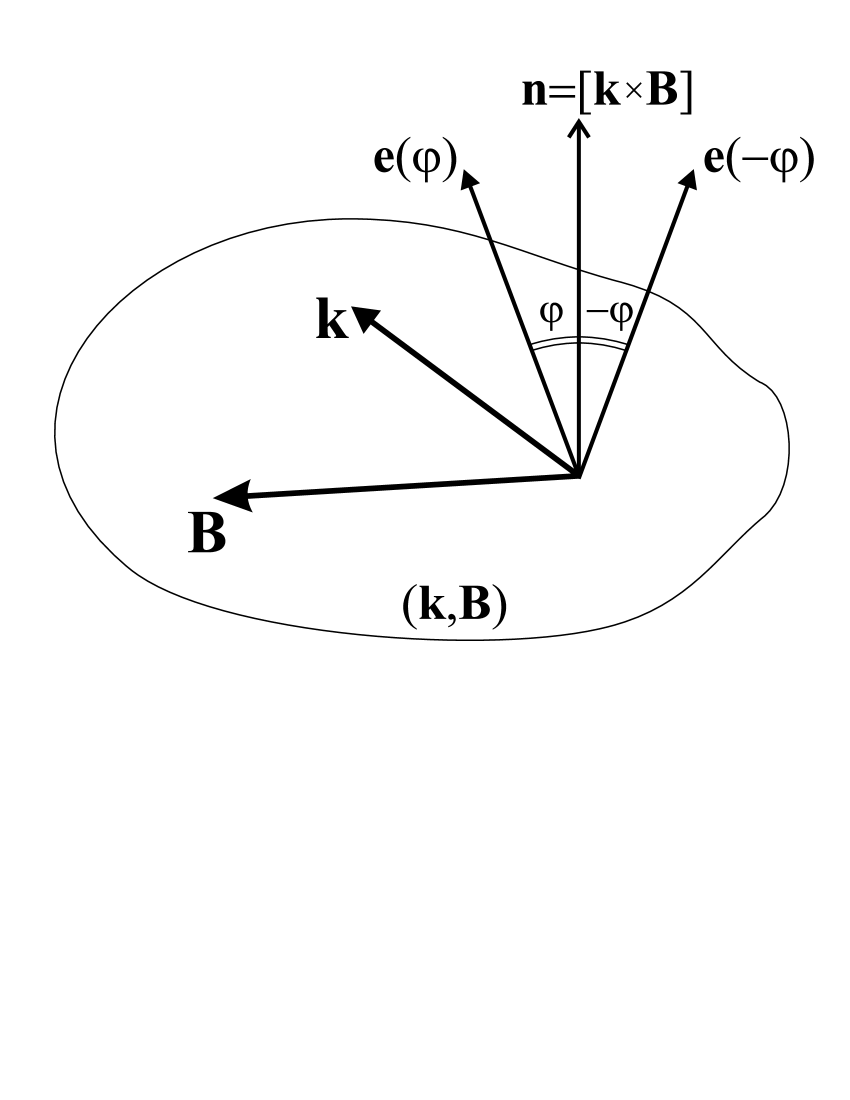
Figure 3: Orientation of the magnetic field B, wavevector k and polarization e of the optical field.

Consider a configuration shown in Fig. 3, where the light field has e($\varphi$ polarization ). Let us perform a mathematical reflection in relation to the plane (${\bf k},{\bf B}$). This leads to the substitution of the polarization vector e($\varphi$)$\to$($-{\bf e}$($-\varphi$)), but for the pseudovector of the magnetic field it leads to ${\bf B}$$\to$($-{\bf B}$). It is known, that the mathematical reflection does not affect a scalar signal, i.e. another relationship is obtained:

$$S({\bf e}(\varphi),{\bf B})=S(-{\bf e}(-\varphi),-{\bf B})\,.$$ (8)

By combining (7) and (8) we finally achieve

$$S({\bf e}(\varphi),{\bf B})=S({\bf e}(-\varphi),{\bf B})\,,$$ (9)

i.e. the scalar signal is an even function of the angle $\varphi$. It means that the points $\varphi$=0,$\,\pi$ (i.e. ${\bf e}$$\perp$${\bf B}$) correspond to the local extremum (maximum or minimum) of the $S({\bf e}(\varphi),{\bf B})$ dependence, which is obtained by rotating the polarization vector ${\bf e}$ around wavevector ${\bf k}$. Similar symmetry consideration shows that there are two other extremuma when the vector ${\bf e}$ lies in the plane (${\bf k},{\bf B}$), i.e., at $\varphi$=$\pm\pi/2$. Note, that the derived results remain valid in the case of light wave propagation (including the nonlinear effects in an optically thick medium). In this case the used above vector e($\varphi$) corresponds to the initial linear polarization before atomic medium (cell).

Thus, we have shown that the described principle of EIT vector magnetometery is valid, in essence, for arbitrary atoms, lines ($D_{1}$ or $D_{2}$), and arbitrary spectral composition of linearly polarized wave (including a monochromatic wave). However, the dependence $A_{\bf k}$($\varphi$) for the central resonance excited by a bichromatic field at the ⁸⁷Rb $D_{1}$ line is the best choice for the demonstration of the compass principle because of the significant signal$/$noise ratio and transmission.

EIT vector magnetometry in a circularly polarized light has been discussed in Wynands2 ; Lee . In those schemes the mathematical models (density matrix and Maxwell equations) are required to reconstruct the vector of the magnetic field from experimental signals. Meanwhile, any model is sensitive to the ultimate knowledge of involved parameters and processes, such as: light intensities, one-photon detunings, light beam profile, atomic density, atomic diffusion motion in buffer gas, collision processes (depolarization, broadening, shifts), and so on. This may limit and sufficiently decrease the achievable angular accuracy (to the level of 1-10 deg) of the vector magnetometer. In contrast, our 3D compass does not require the use of mathematical models, because the extremum of the angle dependence $A_{\bf k}$($\varphi$) at the points $\varphi$=0,$\,\pi$ is an inherent feature.

IV EIT scalar magnetometer

As was shown above, rotating the linear polarization ${\bf e}$ around the wavevector ${\bf k}$ and analyzing the corresponding dependence of amplitude $A_{\bf k}$($\varphi$) of the central dark resonance, we always can find the condition ${\bf e}$$\perp$${\bf B}$. In this section we will consider two end magnetically sensitive resonances (Fig. 2, red solid line), which are connected with $\Lambda_{3,4}$-systems shown in Fig. 1b (i.e. with two-photon transitions $(-1)$$\leftrightarrow$$(-1)$ and $(+1)$$\leftrightarrow$$(+1)$). In the ${\bf e}$$\perp$${\bf B}$ case, the amplitudes of these resonances attain maximum too, because at the exact two-photon resonance (i.e. $\delta_{R}$=$\pm 2g$$\mu_{B}$$|{\bf B}|$/$\hbar$) there are the following two dark states:

$$|dark\rangle_{\Lambda_{3,4}}=\frac{\sqrt{3}E_{2}|F_{1},m=\mp 1\rangle\pm E_{1}|F_{2},m=\mp 1\rangle}{\sqrt{|E_{1}|^{2}+3|E_{2}|^{2}}}.$$ (10)

We can determine the value $|{\bf B}|$ by measuring the distance between these resonances $|\Delta_{\pm}|$. In the linear approximation for $|{\bf B}|$ we apply the formula $|\Delta_{\pm}|$=$\gamma^{\prime}$$|{\bf B}|$, where $\gamma^{\prime}$=$2(g_{F_{2}}-g_{F_{1}})$$\mu_{B}$$/$$\hbar$ is an effective gyromagnetic ratio. Due to the effect of the nuclear magneton for ⁸⁷Rb Arimondo77 ; steck we should use the following values for $g$-factors: $g_{F_{1}}$=$-$0.501827 and $g_{F_{2}}$=0.499836. Thus, in our case $\gamma^{\prime}$=2.803905$\times$10¹⁰ Hz$/$T.

Taking into account the symmetry of the atom-light interactions in the linear polarization one can predict some important properties of such magnetometry scheme. Indeed, this frequency-differential magnetometer is immune to:
(I) the collisional shift arising due to interactions with an isotropic buffer gas;
(II) the quadratic Zeeman shift of magnetic sublevels;
(III) the shift arising from atom-atom interactions (including spin-exchange) between atoms (here between ⁸⁷Rb atoms);
(IV) the ac-Stark shift.

The property (I) is a result of the equality of the collisional shifts of all Zeeman sublevels $|F,m\rangle$ (for a given $F$) in an isotropic buffer gas. The property (II) is also quite obvious considering that each even (on $|{\bf B}|$) power of the Zeeman shift has an equal value and sign for the $m$$\leftrightarrow$$m$ and ($-m$)$\leftrightarrow$($-m$) transitions. This feature is valid for any atom (i.e. not only for ⁸⁷Rb) and line ($D_{1}$ and $D_{2}$).

The property (III) is a result of the interaction of atoms with linear polarized light. Indeed, let us consider the atomic density matrix $\widehat{\rho}$, which describes the distribution among Zeeman sublevels:

$$\widehat{\rho}=\sum_{F^{\prime},m^{\prime},F^{\prime\prime},m^{\prime\prime}}\rho^{F^{\prime}F^{\prime\prime}}_{m^{\prime}m^{\prime\prime}}|F^{\prime},m^{\prime}\rangle\langle F^{\prime\prime},m^{\prime\prime}|\,,$$ (11)

where $\rho^{F^{\prime}F^{\prime\prime}}_{m^{\prime}m^{\prime\prime}}$ are matrix elements. We denote the atomic distribution for two-photon resonances $(+1)$$\leftrightarrow$$(+1)$ and $(-1)$$\leftrightarrow$$(-1)$ (at the $\delta_{R}$=$\pm g\mu_{B}|{\bf B}|$) as $\rho^{(+)F^{\prime}F^{\prime\prime}}_{m^{\prime}m^{\prime\prime}}$ and $\rho^{(-)F^{\prime}F^{\prime\prime}}_{m^{\prime}m^{\prime\prime}}$ respectively. From the general symmetry and neglecting some insignificant details (for example a small variation of the one-photon detuning) we get $|\rho^{(+)F^{\prime}F^{\prime\prime}}_{m^{\prime}m^{\prime\prime}}|$=$|\rho^{(-)F^{\prime}F^{\prime\prime}}_{-m^{\prime}-m^{\prime\prime}}|$. Obviously, this relationship is not changed by the atom-atom interactions (including the spin-exchange process). Therefore, the corresponding collisional frequency shifts have the same magnitude, i.e. they do not affect the frequency difference $\Delta_{\pm}$ (while the collisional broadening of the EIT-resonances will have an influence). This property gives a significant advantage in comparison with other schemes of atomic magnetometers, where the atom-atom interaction is a limiting factor for precise magnetic field measurements. The property (III) supports also the use of miniature size cells in our EIT magnetometer, because it is possible to work at high cell temperature to get high atomic density.

Note that the property (III) can be extended to an arbitrary element (i.e. not only ⁸⁷Rb) and resonance line, when the magnetometer uses the frequency difference between two-photon resonances $m$$\leftrightarrow$$m$ and $(-m)$$\leftrightarrow$$(-m)$. In general, the angle $\theta$ (between vectors ${\bf B}$ and ${\bf e}$) can be arbitrary.

The property (IV) follows from two circumstances. Firstly, the light shifts of two-photon resonances (see Fig. 2, the red solid line) that occur via upper level $F_{e}$=1 are absent, because the dark states nullify the resonant interaction (1). Therefore, these ac-Stark shifts are small and appear mostly due to the interaction with the far-off-resonance level $F_{e}$=2, see Fig. 1. Secondly, due to the symmetry, these shifts are practically identical and compensate each other (in the value $\Delta_{\pm}$). There is, however, a small disbalance caused by Zeeman splitting ($\Delta_{Z}$). This splitting leads to a small difference for all one-photon detunings near the dark resonances $(+1)$$\leftrightarrow$$(+1)$ and $(-1)$$\leftrightarrow$($-1$). Thus, if the value of the light shift for extreme resonances is approximately $U$, then the relative shift can be estimated as $\sim$$|\Delta_{Z}/\delta_{hfs}|$$|U|$, which means an additional significant suppression of shift by the factor $|\Delta_{Z}/\delta_{hfs}|$$\ll$1. Note, that similar advantages of the optically pumped balance magnetometer also has been pointed in Alexandrov3 .

In our case the magnetometer sensitivity $\delta B$ depends on the signal-to-noise ratio (S/N) of the Zeeman resonance signal and the width of the EIT resonance $\Gamma_{\tiny\mbox{FWHM}}$: $\delta B={\Delta B}/(S/N)$, where $\Delta B$=$\Gamma_{\tiny\mbox{FWHM}}$$/$$\gamma^{\prime}$. Therefore, a high contrast of the $\Lambda$-resonances, where most of the atoms ((50-70)$\%$) are accumulated in the dark state icono05 ; lin||lin JETP ; Serezha , makes them a perspective competitor for existing all-optical magnetometers Alexandrov . As an example, we estimate the achievable sensitivity using recently published data on the lin$||$lin resonances Evelina (authors of Evelina characterized the lin$||$lin resonances as an atomic clock reference). With a resonance width $\Gamma_{\tiny\mbox{FWHM}}$=900 Hz and $S/N$=3300 Hz^1/2, the sensitivity for the measurable magnetic field is $\delta{B}<10^{-11}$ T$/$Hz^1/2, which can be obtained without special efforts and for very moderate density $10^{10}$ cm^-3 of rubidium atoms (50 C^∘ and 1.2 Torr $N_{2}$ pressure in Evelina ). To significantly improve the sensitivity one should increase the number of atoms. In this case the EIT differential magnetometer will achieve sensitivity at the level $\delta{B}\sim 10^{-13}$-10^-14 T$/$Hz^1/2 or better, because we expect to reach an atom concentration greater than $10^{12}$ cm^-3 without serious limitations due to collisional processes (property (III)). The proper choice of buffer gas pressure and the additional narrowing of EIT resonance in dense media Mikhailov ; Lukin also gives some advantages. However, it is worth noting that the behavior of the coherent effects (EIT) in dense vapor $>$$10^{12}$ cm^-3 has not yet been studied in detail, though it is known that at $10^{14}$ cm^-3 EIT is still observed Matsko2 .

Additionally we note that each of $\Lambda_{3}$ and $\Lambda_{4}$ resonances (i.e. $(-1)$$\leftrightarrow$$(-1)$ and $(+1)$$\leftrightarrow$($+1$) two-photon transitions) can be used also in the compass scheme (described in the previous section). But it has some drawbacks in comparison with the compass based on the central resonance (i.e. $\Lambda_{1,2}$). Firstly, the frequency position of each of these resonances depends on the magnetic field. Secondly, their transmission dependence $A_{\bf k}$($\varphi$) vs rotation of the vector $\mathbf{e}(\varphi)$ can have two local maximum. One of them (which always exists) corresponds to the case ${\bf e}$$\perp$${\bf B}$, but the other possible maximum emerges, when the vector ${\bf e}$ lies in the plane (${\bf k}$,${\bf B}$). Such situation leads to an uncertainty in the measurement procedure.

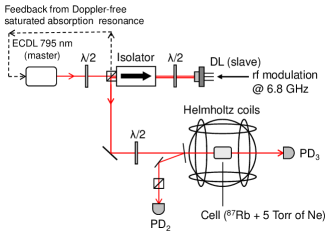
Figure 4: The schematic of the experimental setup.

V Experiment

From our point of view the possibility of an EIT-based compass is the most attractive and unusual part of the suggested ideas. Therefore, in the experimental part we just concentrate on this idea. The experimental setup is shown in Fig. 4. The bichromatic field $\mathbf{E}(\mathbf{r},t)$ is delivered by an extended cavity (ECDL), frequency is modulated at $\Delta_{hfs}$=6.8 GHz and injected into the slave diode laser DL lin||lin JETP . The experiment is carried out on a Pyrex cell (40 mm long and 25 mm in diameter) containing isotopically enriched ⁸⁷Rb and 5 Torr neon buffer gas. The cell is placed inside Helmholtz coils, where the field inhomogeneity is $\sim$2 mG/cm. For the experiments reported here the cell temperature is 45^∘ C.

The laser frequency is locked to the Doppler-free saturated absorption resonance. The radiation power at the cell front window is 1.5 mW. To excite the $\Lambda_{1,2}$ scheme the carrier frequency is tuned to the $F_{2}=2\rightarrow F_{e}=1$ transition, and the high frequency side-band is tuned to the $F_{1}=1\rightarrow F_{e}=1$ transition. The displayed spectra of the EIT resonances are shown in Fig. 2, where the curves correspond to the ⁸⁷Rb transmission spectra for the two cases $\mathbf{e}$$\parallel$$\mathbf{n}$ and $\mathbf{e}$$\perp$$\mathbf{n}$.

Before entering the cell, light passes through a half-wave plate, which is rotating at a 13 Hz rate. As a result, we detect the dependence of light transmission as a function of the angle $\varphi$ between $\mathbf{e}$ and ${\bf n}$, see Fig. 5. It is worth noting that the light transmission is affected by changes of the EIT transmission and by variation of the Doppler absorption profile due to optical pumping. To avoid this distortion of the transmission we detect signals at the second harmonic of the rf-modulated polarization which is done by Faraday modulator at 7.6 kHz. To determine the detection sensitivity of the vector $\mathbf{B}$ direction we change the orientation of the magnetic field in $0.1^{\circ}$ steps. The lock-in amplifier output detects these steps, from which we estimate a sensitivity of $\sim$$10^{-3}$ deg$/$Hz^1/2 (Fig. 6). These data were taken for ${\bf B}\perp{\bf k}$ at 1 G magnetic field with the detection bandwidth of 300 Hz.

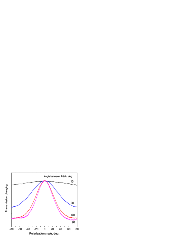
Figure 5: The dependence of the EIT-resonance amplitude $A_{\bf k}$($\varphi$) for the ⁸⁷Rb cell transmission on the angle $\varphi$ between $\mathbf{e}$ and $\mathbf{n}$. Angles between $\mathbf{B}$ and $\mathbf{k}$ are shown on the right side of each curve (both vectors lie in the horizontal plane).

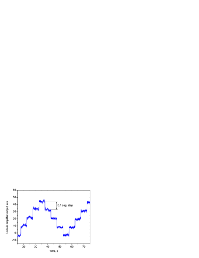
Figure 6: The lock-in amplifier output at $0.1^{\circ}$ angle step variation of the magnetic field direction. The magnetic field magnitude is 1 G, and the angle between magnetic field and wave vector is varied near 90^∘.

Figure 7: Compass sensitivity vs. magnetic field magnitude.

We have found that the sensitivity depends on the magnitude of the applied magnetic field (Fig. 7). At low magnetic field the sensitivity decreases almost by two orders of value compared to that at 0.1-7 G. This occurs due to trap states belonging to the degenerate Zeeman sublevels of the same hyperfine level where atoms ‘‘hide’’. The contrast (as well as signal/noise ratio) grows with the magnetic field. It is caused by lifting of the sublevel degeneracy. To destroy trap states, a magnetic field should be strong enough, i.e. such that the splitting between the ($0$-$0$) (i.e. $\Lambda_{1,2}$) and ($1$-$1$) (i.e. $\Lambda_{3,4}$) transitions greater than the EIT resonance width. Once the ($0$-$0$) and ($1$-$1$) transitions are separated by $\sim$0.1 G (in our setup), the compass has the best sensitivity for $|{\bf B}|$$>$1 G. For some magnetic field ($|{\bf B}|$$>$5 G in our experiments) the central resonance begins to split icono05 ; lin||lin JETP ; Serezha ; Kazakov , because the $\Lambda_{1}$ and $\Lambda_{2}$ transitions have a small difference in $g$-factors ($\pm$2.8 kHz/G) due to the nuclear spin. However, this effect itself does not set the upper operational limit of the magnetic field for the vector measurements (compass), because in this case we can work with one of the two separated $\Lambda$-resonances. We believe that the upper limitation on the magnetic field in our method is connected with the degradation of EIT-resonances when the value $\mu_{B}$$|{\bf B}|$ is comparable with excited state hyper-fine splitting $\delta_{hfs}$$\approx$812 MHz, i.e. due to a strong magnetic mixing between upper hyperfine levels $F_{e}$=1 and $F_{e}$=2 (see Fig. 1). In summary, for the parameters of our setup the magnetic field operational range of the 3D compass is about $\sim$0.1-200 G.

VI Conclusion

In conclusion, we have developed the generalized principles of atomic vector magnetometery based on high-contrast EIT-resonances in a linearly polarized field. These principles follow from a general symmetry of the problem and are valid for arbitrary atoms, transitions, and arbitrary spectral composition of linearly polarized wave (including a monochromatic wave). The compass involving two non-parallel laser beams allows to measure the orientation of the magnetic field in three dimensions. In our proof-of-principle experiment we have achieved a compass sensitivity $\sim$$10^{-3}$ deg/Hz^1/2 at intermediate magnetic fields. We have found that the major contribution to the noise limiting sensitivity is related to intensity fluctuations of the laser system. Thus, we believe that the proposed method has a potential to achieve an angular sensitivity at the level of $\sim$$10^{-4}$ deg/Hz^1/2. In contrast to other schemes of the vector EIT magnetometer, the proposed scheme does not depend on a completeness of the magnetometer mathematical model and gives a straight way to find the magnetic field direction and at the end provides a higher angular accuracy.

We have also discussed properties and advantages of the EIT scalar magnetometry, such as non-sensitivity to quadratic Zeeman and ac-Stark effects, atom-buffer gas and atom-atom collisions. Moreover, our scalar magnetometer works with a maximal sensitivity and an accuracy at the arbitrary mutual orientation of the vectors ${\bf k}$ and ${\bf B}$, i.e. ‘‘dead’’ zones are absent (see also Romalis3 ). The spatial resolution, sensitivity, dynamical range, bandwidth of the magnetic field measurement can be varied by the proper choice of the cell volume, temperature, buffer gas type and its pressure (or coating).

EIT vector magnetometers is important for non-invasive biomedical studies Bison1 ; Bison2 , including the temporal and spacial distribution of the brain and heart electrical currents. Recent successes in the development of chip-sized atomic clocks and magnetometers magnetometry provide a legitimate optimism for the creation of a small size magnetic sensor. As a whole, the proposed EIT compass-magnetometer could find a broad variety of applications in physics, navigation, geology, biology, medicine, and industry.

We thank L. Hollberg, H. Robinson, J. Kitching, F. Levi, S. Knappe, V. Shah, V. Gerginov, P. Schwindt, R. Wynands, I. Novikova, E. Mikhailov, Shura Zibrov and Yiwen Chu for helpful discussions. V.I.Yu. and A.V.T. were supported by RFBR (08-02-01108, 10-02-00591, 10-08-00844) and programs of RAS. V.L.V. and S.A.Z. were supported by RFBR (09-02-011151).

V. I. Yudin e-mail address: viyudin@mail.ru

S. A. Zibrov e-mail address: serezha.zibrov@gmail.com

References

- (1) G. Alzetta, A. Gozzini, L. Moi, and G. Orriols, Il Nuovo Cim. 36B, 5 (1976).
- (2) E. Arimondo, in Progress in Optics, ed. by Wolf E., Vol. XXXV, 257 (1996).
- (3) S. E. Harris, Physics Today 50(7), 36 (1997).
- (4) M. Fleischhauer, M. A. Imamoglu, and J. P. Marangos, Rev. Mod. Phys. 77, 633 (2005).
- (5) M. Fleischauer and M. O. Scully, Phys. Rev. A 49, 1973 (1994).
- (6) S. Pustelny, J. Kimball, S. M. Rochester, V. V. Yashchuk, W. Gawlik, and D. Budker, Phys. Rev. A 73, 23817 (2006).
- (7) I. Novikova, A. B. Matsko, V. L. Velichansky, and G. R. Welch, Phys. Rev. A 56, R1063 (2001).
- (8) M. Sthler, S. Knappe, C. Affolderbach, W. Kemp and R. Wynands, Europhys. Lett. 54, 323 (2001).
- (9) C. Affolderbach, M. Sthler, S. Knappe, and R. Wynands, Appl. Phys. B 75, 605 (2002).
- (10) V. Acosta, M. P. Ledbetter, S. M. Rochester, D. Budker, D. F. J. Kimball, D. C. Hovde, W. Gawlik, S. Pustenly, J. Zachorowski, and V. V. Yashchuk, Phys. Rev. A 73, 053404 (2006).
- (11) D. Budker and M. Romalis, Nature Physics, 3, 227 (2007).
- (12) I. K. Komonis, T. W. Kornack, J. C. Allred, and M. V. Romalis, Nature (London) 422, 596 (2003).
- (13) A. J. Fairweather and M. J. Usher, J. Phys. E 5, 986 (1972).
- (14) E. B. Alexandrov, M. V. Balabas, V. N. Kulyasov, A. E. Ivanov, A. S. Pazgalev, J. L. Rasson, A. K. Vershovski, and N. N. Yakobson, Meas. Sci. Technol. 15, 918 (2004).
- (15) O. Gravrand, A. Khokhlov, J. L. Le Moul, and J. M. Lger, Earth Planets Space 53, 949-958, (2001).
- (16) R. Wynands, A. Nagel, S. Brandt, D. Meschede, and A. Weis, Phys. Rev. A 58, 196 (1998).
- (17) H. Lee, M. Fleischhauer, and M. O. Scully, Phys. Rev. A 58, 2587 (1998).
- (18) D. Budker and M. Romalis, Nature Physics 3, 227 (2007).
- (19) E. B. Alexandrov and A. K. Vershovskii, Phys. Usp. 52, 573 (2009).
- (20) A. V. Taichenachev, V. I. Yudin, V. L. Velichansky, A. S. Zibrov, and S. A. Zibrov, Phys. Rev. A 73, 013812 (2006).
- (21) S. A. Zibrov, Y. O. Dudin, V. L. Velichansky, A. V. Taichenachev, V. I. Yudin, Abstract Book and Technical Digest of ICONO’05 (St. Petersburg, Russia, 11-15 May 2005), ISK8 (2005).
- (22) A. V. Taichenachev, V. I. Yudin, V. L. Velichansky, and S. A. Zibrov, JETP Lett. 82, 449 (2005).
- (23) S. A. Zibrov, V. L. Velichansky, A. S. Zibrov, A. V. Taichenachev, and V. I. Yudin, JETP Lett. 82, 477 (2005).
- (24) E. Breschi, G. Kazakov, R. Lammegger, B. Matisov, L. Windholz, and G. Mileti, IEEE Transactions on Ultrasonics, Ferroelectrics, and Frequency Control 56, 926 (2009).
- (25) S. A. Zibrov, I. Novikova, D. F. Phillips, R. L. Walsworth, A. S. Zibrov, V. L. Velichansky, A. V. Taichenachev, and V. I. Yudin, Phys. Rev. A 81, 013833 (2010).
- (26) E. E. Mikhailov, T. Horrom, N. Belcher, and I. Novikova, J. Opt. Soc. Am. B 27, 417 (2010).
- (27) E. Arimondo, M. Inguscio, and P. Violino, Rev. Mod. Phys. 49, 31 (1977).
- (28) D. A. Steck, ‘‘Rubidium 87 D Line Data’’, available online at http://steck.us/alkalidata (revision 2.0.1, 2 May 2008).
- (29) E. B. Alexandrov, A. B. Mamyrin, and A. P. Sokolov, Optika i Spektroskopiya (USSR) 34, 1216 (1973).
- (30) M. D. Lukin, M. Fleischhauer, A. S. Zibrov, H. G. Robinson, V. L. Velichansky, L. Hollberg, and M. O. Scully, Phys. Rev. Lett. 79, 2959 (1997).
- (31) E. E. Mikhailov, V. A. Sautenkov, Yu. V. Rostovtsev, A. Zhang, M. S. Zubairy, M. O. Scully, and G. R. Welch, Phys. Rev. A 74, 013807 (2006).
- (32) A. S. Zibrov, A. B. Matsko, L. Hollberg, and V. L. Velichansky, J. Mod. Opt. 49, 359 (2002).
- (33) G. Kazakov, B. Matisov, I. Mazets, G. Mileti, and J. Delporte, Phys. Rev. A 72, 063408 (2005).
- (34) A. Ben-Kish and M. V. Romalis, arXiv:1001.0345 (2010).
- (35) G. Bison, R. Wynands, and A. Weis, Appl. Phys. B 76, 325 (2003).
- (36) G. Bison, R. Wynands, and A. Weis, Opt. Expr. 11, 904 (2003).
- (37) P. Schwindt, S. Knappe, V. Shah, L. Hollberg, J. Kitching, L. Liew, and L. Moreland, Appl. Phys. Lett. 85, 6409 (2004).