Non-Abelian Gauge Field Localized on
Walls with Four-Dimensional World Volume

Abstract

A mechanism using the position-dependent gauge coupling is proposed to localize non-Abelian gauge fields on domain walls in five-dimensional space-time. Low-energy effective theory posseses a massless vector field, and a mass gap. The four-dimensional gauge invariance is maintained intact. We obtain perturbatively the four-dimensional Coulomb law for static sources on the domain wall. BPS domain wall solutions with the localization mechanism are explicitly constructed in the $U(1)\times U(1)$ supersymmetric gauge theory coupling to the non-Abelian gauge fields only through the cubic prepotential, which is consistent with the general principle of supersymmetry in five-dimensional space-time.

1 Introduction

Besides supersymmetric theories, [1] the most intriguing possibilities for unified theories beyond the standard model are models with extra dimensions, that is, the brane-world scenario [2, 3, 4]. In this scenario, our four-dimensional world is localized on defects (which are often called branes) such as domain walls in a higher-dimensional space-time, and the standard model particles are assumed to be localized on the defect. Domain walls are the simplest defect and have been most useful to construct realistic models. However, localization of gauge fields on domain walls has been notoriously difficult in field theories, although scalar and spinor fields have been successfully localized. It has been recognized early that the model with the warp factor does not help to localize the gauge field on the domain wall. [5, 6] More recently it was proposed that bulk and boundary mass terms can be introduced into a warped model to help localize gauge fields. [7] It was achieved at the cost of a subtle fine-tuning as well as certain boundary interactions to restore the gauge invariance. An explicit model of Abelian gauge field localized on a domain wall in five-dimensional space-time has been obtained using tensor multiplet [8]. However, it has been difficult to extend the idea of tensor multiplet to incorporate the non-Abelian local gauge symmetry. If we are content with toy models of lower-dimensional world-volume, such as domain walls with the three-dimensional world-volume, there have been a number of proposals, assuming nonperturbative effects [9], or using perturbative methods [10, 11]. However, it has been difficult to obtain an explicit model of non-Abelian gauge fields localized on a domain wall in five-dimensional space-time.

A basic problem has been pointed out to localize gauge fields on a domain wall [9, 3]. We wish to obtain a (perturbatively) unbroken gauge symmetry on the world volume of the domain wall. Since one wishes to prevent gauge fields to propagate freely in the bulk, one is tempted to consider that the bulk space-time outside of the domain wall to be in the Higgs phase where gauge symmetry is broken. Unfortunately, however, the flux coming out of the source on the domain wall is absorbed by the bulk in the Higgs phase and cannot reach beyond the width of the domain wall even in the direction along the world volume of the domain wall. Because of this screening effect, the vector field acquires a mass of the order of the inverse width of the wall [9, 3, 8, 12]. On the contrary, if a vector field is confined in the bulk and deconfined on the domain wall, the flux coming out of a source should be expelled from the bulk, producing the four-dimensional Coulomb law on the world volume of the domain wall. Therefore we need to consider the confining phase for the bulk, whose explicit implementation is often difficult. This difficulty is particularly acute in our problem, since a realistic model requires the five-dimensional bulk, where the knowledge on nonperturbative effects is scarce. Nonperturbative effects in a five-dimensional gauge theory with a cut-off was proposed to obtain the layered phase that confines only along the extra dimension[13].

Even if the detailed knowledge of nonperturbative effects is not available, the confining medium can be rephrased classically by introducing a dielectric permeability $\epsilon$ for gauge fields[14, 15]. In the classical electrodynamics of a dielectric medium, the electric flux density $\boldsymbol{D}$ is the sum of the electric field $\boldsymbol{E}$ and the polarization $\boldsymbol{P}$ induced by $\boldsymbol{E}$

$$\boldsymbol{D}=\epsilon_{0}\boldsymbol{E}+\boldsymbol{P}\equiv\epsilon\boldsymbol{E}$$ (1)

where the permeability $\epsilon(\boldsymbol{x})$ depends on the spatial position $\boldsymbol{x}$, and the vacuum permeability is denoted as $\epsilon_{0}$. For ordinary dielectric media, the dielectric permeability $\epsilon$ is greater than the vacuum permeability $\epsilon_{0}$, since the polarization $\boldsymbol{P}$ is always induced in the same direction as the electric field $\boldsymbol{E}$. On the other hand, it has been proposed that the confining vacuum can be represented by an unusual dielectric permeability $\epsilon\to 0$, namely by a perfect dia-electric medium. A relativistic version of the dielectric permeability can be expressed by a Lagrangian [14] with the field strength $F_{\mu\nu}\equiv\partial_{\mu}W_{\nu}-\partial_{\nu}W_{\mu}$ of an Abelian vector field $W_{\mu}$

$${\cal L}=-{1\over 4}\epsilon(\boldsymbol{x})F_{\mu\nu}F^{\mu\nu}.$$ (2)

The dielectric permeability in this form is nothing but the position-dependent gauge coupling $g^{2}(\boldsymbol{x})$

$$\epsilon(\boldsymbol{x})={1\over g^{2}(\boldsymbol{x})},$$ (3)

and the region of the confining vacuum is represented by the strong coupling $g^{2}\to\infty$ in this classical language. Therefore we can represent the confining vacuum in the bulk and deconfining vacuum on the domain wall classically by the position-dependent gauge coupling, by requiring strong coupling $g^{2}\to\infty$ asymptotically in the bulk away from the domain wall, and weak coupling on the domain wall.

The purpose of our paper is to propose the position-dependent gauge coupling as a model for a gauge field localization on domain walls, to examine its generic properties, and to construct explicit examples of such domain walls as BPS states in supersymmetric gauge theories. The general features of the position-dependent gauge coupling are discussed in §2. We find that the four-dimensional gauge invariance is intact, assuring the existence of massless gauge field in the low-energy effective theory. By analyzing modes of effective fields in four-dimensional world-volume, we find that our model indeed has a massless gauge field and a mass gap. It is worth stressing that this mechanism is applicable to localization of the non-Abelian gauge fields as well as the Abelian gauge field. We will discuss these points in §3. We also show in §4 that the gauge field localized on the domain wall exhibits perturbatively a four-dimensional Coulomb law for static sources localized on the world volume of the domain wall. As explicit examples, we construct BPS domain wall solutions in supersymmetric gauge theories with $U(1)\times U(1)$ gauge group in §5. The non-Abelian gauge fields couple to these $U(1)\times U(1)$ vector multiplets only through the cubic prepotential and are localized on the domain wall. It is remarkable that the cubic coupling among vector multiplets is just sufficient to give a nontrivial profile of position-dependent coupling function automatically, once the domain wall is formed as the background solution. This satisfies the stringent constraint of supersymmetric gauge theories in five-dimensional space-time allowing only up to cubic coupling in the prepotential of vector multiplets [16]. We will discuss briefly mechanisms to introduce matter multiplets in the nontrivial representations of the localized non-Abelian gauge fields in §6.

2 A model of position-dependent gauge coupling

In this section, we will explore general features of localized gauge fields on domain walls, without relying on a particular form of domain wall solutions. Concrete examples of domain wall solutions demonstrating the feasibility of our mechanism of localization will follow in later sections. We consider a domain wall in $4+1$ dimensional space-time, whose coordinates are denoted by $x^{M},M=0,1,\cdots,4$, whereas the world-volume coordinates and the codimension of the domain wall are denoted as $x^{\mu},\mu=0,1,2,3$, and $y$, respectively. Namely the domain wall profile depends only on $y$. We assume that the five-dimensional gauge field acquires a position-dependent gauge coupling function $\epsilon(y)$, on the background domain wall solution. We normalize the position-dependent gauge coupling function $\epsilon(y)$ as

$$\int_{-\infty}^{\infty}dy\,\epsilon(y)=\frac{1}{g_{4}^{2}},$$ (4)

and denote the four-dimensional gauge coupling as $g_{4}$. Let us first consider gauge field $W_{M}^{a}$ with non-Abelian gauge group $G$, where $a$ runs from 1 to $\dim G$, in $4+1$-dimensional space-time. Denoting the source and the field strength as $J_{M}$ and $F^{a}_{MN}\equiv\partial_{M}W_{N}^{a}-\partial_{N}W^{a}_{M}-f^{abc}W^{b}_{M}W^{c}_{N}$ with $M,N=0,1,\cdots,4$, we take the following Lagrangian with the position-dependent gauge coupling function $\epsilon(y)$ instead of the ordinary five-dimensional gauge coupling constant $1/g_{5}^{2}$

$${\cal L}=-\frac{1}{4}\epsilon(y)F^{MNa}F^{a}_{MN}.$$ (5)

Our metric convention is $\eta_{MN}={\rm diag.}(+,-,\cdots,-)$.

We assume that the position-dependent gauge coupling function $\epsilon(y)$ is real and nonnegative everywhere

$$\epsilon(y)>0.$$ (6)

and has a profile localized on a domain wall. Let us take the center of the domain wall to be at $y=0$. We make a crucial assumption for $\epsilon(y)$ to vanish at both infinity $y\to\pm\infty$

$$\epsilon(y)\to 0,\qquad y\to\pm\infty.$$ (7)

This asymptotic behavior represents the strong coupling in the bulk, namely the confining vacuum. It has been proposed that this type of “a perfect dia-electric medium” is the classical representation of confining vacuum [14, 15].

The Lagrangian (5) gives the field equation

$$0=\epsilon(y)(D^{N}F_{NM})^{a}+(\partial^{y}\epsilon(y))F^{a}_{yM},$$ (8)

where $(D^{N}F_{NM})^{a}\equiv\partial^{N}F^{a}_{NM}-f^{abc}W^{Nb}F^{c}_{NM}$ and we have used the fact that the position-dependent gauge coupling function depends only on $y$. By analyzing the field equation (8), we will explore the low-energy effective field theory in four-dimensional space-time in the following sections.

3 Mode Analysis

In this section, we would like to find massless and massive modes that appear in the low-energy effective field theory of the five-dimensional gauge theory with the position-dependent gauge coupling function $\epsilon(y)$. We first need to obtain mode functions using the linearized field equation arising from quadratic terms of the Lagrangian (5). We can define a mode expansion of the Lagrangian assuming these mode functions are complete, provided they are normalizable. The linearized field equation is given by

$$0=\epsilon(y)(\partial^{N}\partial_{N}W^{a}_{M}-\partial^{N}\partial_{M}W^{a}_{N})+(\partial^{y}\epsilon(y))(\partial_{y}W^{a}_{M}-\partial_{M}W^{a}_{y}).$$ (9)

To find mode functions, we here choose an axial gauge

$$W^{a}_{y}=0.$$ (10)

Then the field equation (9) for $M=\mu$ component becomes

$$0=\epsilon(y)\left\{(\partial^{\nu}\partial_{\nu}-\partial_{y}^{2})W^{a}_{\mu}-\partial_{\mu}\partial^{\nu}W^{a}_{\nu}\right\}-\partial_{y}\epsilon(y)\partial_{y}W^{a}_{\mu}.$$ (11)

Operating by $\partial^{\mu}$ to the above field equation, we find

$$0=-\partial_{y}\left(\epsilon(y)\partial_{y}(\partial^{\mu}W^{a}_{\mu})\right).$$

Thus $\partial^{\mu}W^{a}_{\mu}$ separates variables $x$ and $y$, and factorizes into

$$\partial^{\mu}W^{a}_{\mu}=Y(y)F^{a}(x),$$ (12)

where we define

$$Y(y)=\int^{y}dy^{\prime}\frac{1}{\epsilon(y^{\prime})},$$ (13)

and $F^{a}(x)$ is a function of $x$ only. Therefore we find no propagating modes in the longitudinal part $\partial^{\mu}W^{a}_{\mu}$. Even though the longitudinal part does not provide a propagating modes, it may contribute to a potential responding to a static source, as is usual in quantum electrodynamics. We will discuss the static potential due to a source in the next section.

Now we decompose $W^{a}_{\mu}$ into transverse and longitudinal components, $W_{\mu}^{aT}$ and $W_{\mu}^{aL}$. In particular, using (12), the longitudinal component reduce to

$$W_{\mu}^{aL} \equiv \frac{1}{\partial^{2}}\partial_{\mu}\partial^{\nu}W^{a}_{\nu}$$ (14)

$$= Y(y)\frac{1}{\partial^{2}}\partial_{\mu}F^{a}(x)$$

Plugging the decomposition $W^{a}_{\mu}=W_{\mu}^{aT}+W_{\mu}^{aL}$ into (11) and using (14), we finally find the field equation for the transverse component $W_{\mu}^{aT}$

$$0=\epsilon(y)\partial^{\nu}\partial_{\nu}W_{\mu}^{aT}-\partial_{y}(\epsilon(y)\partial_{y}W_{\mu}^{aT}).$$ (15)

Let us now expand $W_{\mu}^{aT}$ by a complete set of wave functions $u_{n}(y)$ in $y$ as

$$W_{\mu}^{aT}=\sum_{n}w^{a(n)}_{\mu}(x)u_{n}(y),$$ (16)

where $w^{a(n)}_{\mu}(x)$ satisfies

$$(\partial^{\nu}\partial_{\nu}+m_{n}^{2})w^{a(n)}_{\mu}(x)=0,$$

and $m_{n}$ represents mass of the mode. Plugging the mode expansion (16) into the field equation (15), we find the equation for the mode function $u_{n}(y)$

$$\left[-\frac{1}{\epsilon(y)}\frac{d}{dy}\epsilon(y)\frac{d}{dy}-m_{n}^{2}\right]u_{n}(y)=0.$$ (17)

If we change the variable from $y$ to $Y$ defined in Eq. (13) satisfying $\frac{d}{dY}\equiv\epsilon(y)\frac{d}{dy}$, the mode equation (17) can be transformed into a bound state problem at the threshold (zero energy) for a potential $U(Y)$ which is proportional to the mass squared $m_{n}^{2}$ of the mode

$$H\equiv-\frac{1}{2}\frac{d^{2}}{dY^{2}}+U(Y),\quad U(Y)=-\frac{1}{2}m_{n}^{2}\epsilon^{2}(y(Y)),$$ (18)

$$Hu_{n}(Y)=0.$$ (19)

Let us note that the normalization of the position-dependent coupling function $\epsilon$ is fixed by the four-dimensional gauge coupling $g_{4}$ in Eq. (4)

$$\frac{1}{g_{4}^{2}}=\int dy\,\epsilon(y)=\int dY\,\epsilon^{2}(y(Y)),$$ (20)

where the integration should be carried out over the entire region of $y$ or $Y$.

For a given shape $\epsilon(y(Y))$ of the potential, we can find all possible threshold bound states at various discrete depths of the potential $U(Y)$ by adjusting $m_{n}^{2}$. In this way, finding threshold (zero energy) bound state solutions gives a discrete spectrum of mass squared $m_{n}^{2}$ of modes. We wish to obtain the low-energy effective Lagrangian defined by an integration of the fundamental five-dimensional Lagrangian over $y$

$${\cal L}_{\rm eff}\equiv\int dy\,{\cal L}_{5}.$$ (21)

This effective Lagrangian dictates the normalization condition which naturally contains the following measure $g_{4}^{2}\;\epsilon(y)$ for the mode function

$$\int_{-\infty}^{\infty}dy\,[g_{4}^{2}\;\epsilon(y)]u_{n}(y)^{*}u_{l}(y)=\delta_{nl}.$$ (22)

This measure is a distinctive feature of our threshold bound state mode functions.

We see that constant mode is always a zero energy solution:

$$u_{0}={\rm constant},\quad Hu_{0}=0.$$ (23)

The normalizability of this constant mode is equivalent to the condition of finiteness of the effective four-dimensional gauge coupling in Eq. (20). As will be illustrated by solvable examples in the following, there is a mass gap for these threshold bound states, and their wave functions are normalizable because of the nontrivial measure in Eq. (22), similarly to the constant mode, provided the finite four-dimensional gauge coupling can be defined by Eq. (20). This situation is quite different from the threshold bound states in the usual quantum mechanics problems in one spatial dimension.

To illustrate our procedure of finding the spectrum of modes for the position-dependent gauge coupling, we will take two examples of solvable potentials that can also serve as approximations to our concrete examples of domain wall solutions in subsequent sections.

Solvable Example 1

We first consider the potential

$$U(Y)=-\frac{U_{0}}{\cosh^{2}\alpha Y},$$ (24)

which is plotted in Fig.1(a). Because of the relation (18) and the normalization condition (20), the position-dependent coupling function $\epsilon$ is fixed in this case as

$$\epsilon(Y)=\frac{1}{g_{4}}\sqrt{\frac{\alpha}{2}}\frac{1}{\cosh\alpha Y}.$$ (25)

Then Eq. (13) implies $y=(g_{4}\sqrt{2}/\alpha^{3/2})\sinh\alpha Y$. Therefore, from Eqs.(18) and (24), we find

$$\epsilon(y) = \frac{1}{g_{4}}\sqrt{\frac{\alpha}{4}}\frac{1}{\cosh\alpha Y(y)}=\frac{1}{g_{4}}\sqrt{\frac{\alpha}{4g_{4}^{2}+2g_{4}\alpha^{3}y^{2}}},$$ (26)

which is shown in Fig.1(b).

If we consider the eigenvalue problem $Hv_{k}=E_{k}v_{k}$, we immediately find[17] that the finite number of bound states exist with a discrete energy spectrum $E_{k}=-(\alpha^{2}/2)(s-k)^{2}$, $k=0,1,\ldots\leq s$ with

$$s\equiv{1\over 2}\left(-1+\sqrt{1+\frac{8U_{0}}{\alpha^{2}}}\right)$$ (27)

The threshold bound state $E_{k}=0$ occurs if and only if $k=s$ with $s$ being a nonnegative integer $s=n,n=0,1,2,\ldots$. This gives the $n$-th threshold bound state. In that case, the potential depth $U_{0}$ satisfies

$$U_{0}=\frac{\alpha^{2}}{2}n(n+1).$$ (28)

Eq.(18) implies the threshold bound state spectrum

$$m_{n}^{2} = 2g_{4}^{2}\alpha n(n+1),\qquad n=0,1,2,\ldots.$$ (29)

(a) Potential in $Y$	(b) Position-dependent gauge coupling in $y$

Figure 1: The cosh-type potential and related profile of the coupling function. A dashed line within the coupling function represents the wave function of the localized massless vector field around the domain wall.

First we consider the energy level at $n=0$. This gives the massless mode $m_{0}^{2}=0$, whose wave function turns out to be the constant $u_{0}(y)=1$, as we have seen before. Secondly, the first excited mode gives $m_{1}^{2}=4g_{4}^{2}\alpha$. Similarly, higher excited modes gives larger discrete values of $m_{n}^{2}$. The normalizability (22) of the $n$-th mode in this example is given by the finiteness of

$$\int_{-\infty}^{\infty}dy\,\epsilon(y)|u_{n}(y)|^{2}=\int_{-\infty}^{\infty}dY\,\frac{\alpha}{2g_{4}^{2}\cosh^{2}\alpha Y}|u_{n}(Y)|^{2}.$$ (30)

We find that wave functions of all the excited modes are normalizable, since they are just polynomials[17] in $\tanh\alpha Y$. Thus we conclude that there is a massless mode and a mass gap for the first excited mode, both of which are normalizable. We can safely use the effective field theory of the massless gauge fields below the energy scale $m_{1}$, ignoring the massive modes. The value of the mass gap is proportional to the inverse of the width $\frac{1}{\alpha}$ of the position-dependent coupling function $\epsilon$ and the square of the gauge coupling $g_{4}^{2}$. The massless zero mode wave function including the square root of the measure $\sqrt{\epsilon(y)}u_{0}(y)$ is plotted in Fig.1(b) by a dashed line.

Solvable Example 2

Next solvable example is a square well potential

$$U(Y)=\left\{\begin{array}[]{ll}-U_{0},&|Y|<a\\ 0,&|Y|>a\end{array}\right..$$ (31)

(See Fig.2.) Then, the coupling function is given by

$$\epsilon(Y)=\left\{\begin{array}[]{ll}\frac{\sqrt{2U_{0}}}{m_{n}},&|Y|<a\\ 0,&|Y|>a\end{array}\right..$$

Using the normalization of the profile $\epsilon(y)$, we determine

$$U_{0}=\frac{m_{n}^{2}}{4ag_{4}^{2}}.$$

Energy levels and wave functions for this square well potential can be exactly solved, and the threshold bound states occur when we choose

$$U_{0}=\frac{\pi^{2}}{8a^{2}}n^{2},\qquad n=0,1,2,\ldots.$$ (32)

Therefore the mass spectra of threshold bound states are given by

$$m_{n}^{2}=4g_{4}^{2}aU_{0}=\frac{\pi^{2}}{2a}g_{4}^{2}n^{2}.$$

Again we find there is a massless zero mode at the level $n=0$ and finite mass gaps for higher excited states.

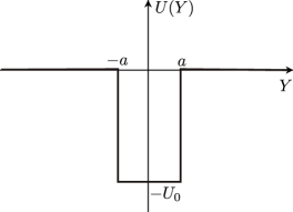
Figure 2: The square well potential with a depth $U_{0}$. There exists a threshold bound state if we choose $U_{0}$ suitably.

4 Four-dimensional Coulomb law

In this section, we wish to demonstrate that the position-dependent gauge coupling in Eq.(5) exhibits the four-dimensional Coulomb law for the static source on the world volume of the domain wall, following a treatment in Ref.Dvali:2000rx. We introduce a source term ${\cal J}^{a}_{M}$ to Eq.(5) to examine the response

$${\cal L}=-\frac{1}{4}\epsilon(y)F^{a}_{MN}F^{aMN}+{\cal J}^{a}_{M}W^{aM}.$$ (33)

We are interested in an external source ${\cal J}_{M}(x,y)$ that is localized on the world volume of the domain wall, and has components only in four-dimensional world-volume:

$${\cal J}^{a}_{M}(x,y)=\delta(y)\delta_{M\mu}J^{a}_{\mu}(x).$$ (34)

The free field equation for the gauge field $W^{a}_{M}$, namely the equation of motion ignoring the nonlinear interaction terms reads

$$0=\epsilon(y)(\partial^{M}\partial_{M}W^{a}_{N}-\partial^{M}\partial_{N}W^{a}_{M})+\partial^{y}\epsilon(y)(\partial_{y}W^{a}_{N}-\partial_{N}W^{a}_{y})-{\cal J}^{a}_{N}.$$ (35)

In this section we choose the Lorentz gauge (in five dimensions)

$$\partial^{M}W^{a}_{M}=0.$$ (36)

Then the field equation becomes

$$0=\epsilon(y)\partial^{M}\partial_{M}W^{a}_{N}+\partial^{y}\epsilon(y)(\partial_{y}W^{a}_{N}-\partial_{N}W^{a}_{y})-{\cal J}^{a}_{N}.$$ (37)

Since the source has no $y$-component, the field equation for the extra-dimensional component $W_{y}$ becomes

$$0=\epsilon(y)\partial^{M}\partial_{M}W^{a}_{y},$$ (38)

without any source term at $y=0$. Because of nonnegative definiteness of $\epsilon(y)$, we find that $W^{a}_{y}$ obeys a free field equation in five dimensions without source. Assuming that there is no external source at infinity, we obtain that there is no nontrivial solution. To demonstrate it, let us solve the free field equation by going to the Euclidean space. Denoting the mixed representation of the momentum space only in four dimensions as $\tilde{W}^{a}_{y}(p,y)$, we obtain

$$0=(p^{2}-\partial_{y}^{2})\tilde{W}^{a}_{y}(p,y).$$ (39)

There are two independent solutions with $C_{+}(p),C_{-}(p)$ as arbitrary functions of $p$

$$\tilde{W}^{a}_{y}(p,y)=C_{+}(p)e^{py}+C_{-}(p)e^{-py},$$ (40)

which is valid in the entire region $-\infty<y<\infty$. Since no external source at infinity requires $\tilde{W}^{a}_{y}(p,y)\to 0$ at both infinities $y\to\pm\infty$, we obtain $C_{+}(p)=C_{-}(p)=0$, which implies no nontrivial solution: $W^{a}_{y}=0$.

Taking account of $W^{a}_{y}=0$ and Eq.(34), we obtain the field equation for $W^{a}_{\mu}$ as

$$0=\epsilon(y)\partial^{\nu}\partial_{\nu}W^{a}_{\mu}+\partial^{y}\left(\epsilon(y)\partial_{y}W^{a}_{\mu}\right)-\delta(y)J^{a}_{\mu}(x).$$ (41)

Now we give a simple example to see the Coulomb law on the domain wall. We assume the weak coupling region (domain wall) is sufficiently thin and the coupling profile behaves as $\epsilon_{\rm thin}(y)=\frac{\delta(y)}{g_{4}^{2}}$.

For regularization purposes, we will add a large, but finite values for the asymptotic bulk gauge coupling

$$\epsilon_{\rm thin}(y)=\frac{\delta(y)}{g_{4}^{2}}+\frac{1}{g_{5}^{2}}.$$ (42)

We consider this simplified situation of the zero-width limit of the domain wall in Eq.(42), and examine the case of the finite width of the domain wall later to confirm that our result is unchanged. Going again to the Euclidean space, and using the mixed representation $\tilde{W}^{a}_{\mu}(p,y)$ of the momentum space only in four dimensions, we obtain the field equation as

$$0=\frac{(p^{2}-\partial_{y}^{2})}{g_{5}^{2}}\tilde{W}^{a}_{\mu}(p,y)+\frac{\delta(y)p^{2}\tilde{W}^{a}_{\mu}(p,y)}{g_{4}^{2}}-\frac{\partial_{y}\left(\delta(y)\partial_{y}\tilde{W}^{a}_{\mu}(p,y)\right)}{g_{4}^{2}}-\delta(y)\tilde{J}^{a}_{\mu}(p).$$ (43)

Since the field equation (43) for $y\not=0$ is identical to the $W^{a}_{y}$ component, we obtain

$$\tilde{W}^{a}_{\mu}(p,y)=C_{\mu}^{a+}(p)e^{-py}\theta(y)+C_{\mu}^{a-}(p)e^{py}\theta(-y).$$ (44)

Integrating the field equation (43) in the infinitesimal interval between $y=-\varepsilon$ and $y=\varepsilon$, we obtain

$$0=-\int_{-\varepsilon}^{\varepsilon}dy\,\frac{\partial_{y}^{2}\tilde{W}^{a}_{\mu}(p,y)}{g_{5}^{2}}+\frac{p^{2}}{g_{4}^{2}}\tilde{W}^{a}_{\mu}(p,y)-\frac{1}{g_{4}^{2}}\int_{-\varepsilon}^{\varepsilon}dy\,\partial_{y}\left(\delta(y)\partial_{y}\tilde{W}^{a}_{\mu}(p,y)\right)-\tilde{J}^{a}_{\mu}(p).$$ (45)

By inserting the solution (44) for $y\not=0$, we find that the absence of divergent terms such as $(\delta(y))^{2}$ in Eq.(45) from the third term $\delta(y)\partial_{y}\tilde{W}^{a}_{\mu}(p,y)$ requires

$$C_{\mu}^{a+}(p)=C_{\mu}^{a-}(p)\equiv C^{a}_{\mu}(p).$$ (46)

With this condition (46), the third term vanishes :

$$-\frac{1}{g_{4}^{2}}\int_{-\varepsilon}^{\varepsilon}dy\,\partial_{y}\left(\delta(y)\partial_{y}\tilde{W}^{a}_{\mu}(p,y)\right)=\frac{pC_{\mu}(p)}{g_{4}^{2}}\int_{-\varepsilon}^{\varepsilon}dy\,\partial_{y}\left(\delta(y)\partial_{y}\left({\rm sgn}(y)e^{-p|y|}\right)\right)=0.$$ (47)

Now the field equation determines the amount of discontinuity $2pC^{a}_{\mu}(p)$ of the derivative of $\tilde{W}^{a}_{\mu}$ at $y=0$ in terms of the source $\tilde{J}^{a}_{\mu}(p)$ leading to

$$\tilde{W}^{a}_{\mu}(p,y=0)=\frac{g_{4}^{2}}{p^{2}+\frac{2g_{4}^{2}}{g_{5}^{2}}p}\tilde{J}^{a}_{\mu}(p).$$ (48)

In the strong coupling limit $g_{5}^{2}\to\infty$ of the bulk asymptotic coupling, we finally obtain

$$\lim_{g_{5}^{2}\to\infty}\tilde{W}^{a}_{\mu}(p,y=0)=\frac{g_{4}^{2}}{p^{2}}\tilde{J}^{a}_{\mu}(p).$$ (49)

If we put a static charge as the source $\tilde{J}^{a}_{\mu}(p)=Q^{a}\delta_{\mu 0}$, we obtain the potential in the coordinate space by a Fourier transformation of (49)

$$W_{\mu}^{a}(x,y=0)=\frac{1}{4\pi}\frac{1}{r}g_{4}^{2}Q^{a}\delta_{\mu 0},$$ (50)

with the three-dimensional spatial distance $r$. Thus we obtain the Coulomb law in four-dimensional world volume as we anticipated.

The intermediate form of our potential in Eq.(48) turns out to be identical to the result in Ref.Dvali:2000rx. However, let us note two important difference of our analysis from that in Ref.Dvali:2000rx. Firstly, we have introduced the bulk asymptotic coupling $g_{5}^{2}$ merely as a regularization parameter, and the agreement of the potential at an intermediate step is somewhat technical. Moreover our starting Lagrangian possesses the five-dimensional field strengths $F^{a}_{MN}$ localized at the wall, in contrast to their Lagrangian in Ref.Dvali:2000rx where only four-dimensional field strengths $F^{a}_{\mu\nu}$ are localized. This difference results in the presence of the third term in Eq.(43). As we noted, this term gives us a consistency condition (46), which does not follow from the field equation in Ref.Dvali:2000rx. Instead they seem to have assumed (quite naturally) a symmetry of $\tilde{W}^{a}_{\mu}(p,y)$ under $y\to-y$. Thanks to this consistency condition, the third term in Eq.(45) vanishes and the resultant potential has become identical to that in Ref.Dvali:2000rx.

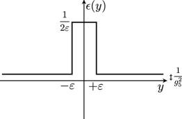
Figure 3: The position-dependent coupling is very thin step function. In the limit of $\varepsilon\to 0$, the position-dependent coupling becomes a delta function. An asymptotic height of $1/g_{5}^{2}$ is introduced for a regularization.

So far we have been studying the zero-width approximation for the domain wall. Let us now examine the case of the finite width of the domain wall by regularizing the delta function profile. As a simplest regularization, we take the following step-function ansatz [18] for the domain wall profile function $\epsilon(y)$ (see Fig.3):

$$\epsilon_{\rm step}(y)\equiv\left\{\begin{array}[]{lr}1/(2\varepsilon)&|y|<\varepsilon\\ 1/g_{5}^{2}&|y|>\varepsilon\end{array}\right..$$ (51)

Since the solution for $W^{a}_{y}$ in Eq.(40) uses only the positive definiteness of the coupling without referring to the $y$-profile of the coupling in Eq.(38), we find that $W^{a}_{y}=0$ even for the finite width case. Moreover, the position-dependent gauge coupling factors out for $y\not=0$, and the source term exists only at $y=0$. Therefore the solution for $y\not=0$ as well as the discontinuity at $y=0$ are unchanged from the zero-width case. We thus find that exactly the same solution (49) is valid in this finite width case. Generally we should obtain somewhat different $y$-profile of the solution for other finite width regularizations. However, our example shows that the qualitative behavior, the four-dimensional Coulomb law particularly, should be the same as the zero-width case. In the case of Ref.Dvali:2000rx, the finite width regularization by the step function gives a solution for $W^{a}_{\mu}$ different from the zero-width limit, contrary to our Lagrangian. This result arises from the fact that our Lagrangian contains the extra-dimensional component of the field strength with the position-dependent coupling $\epsilon(y)$.

5 Supersymmetric models for BPS walls

5.1 General set up

In order to have a realistic brane world with four-dimensional world-volume, we construct a domain wall using five-dimensional supersymmetric gauge theories, which have eight supercharges and consist of vector multiplets and hypermultiplets. We will consider at least two $U(1)$ vector multiplets labeled by $I=1,2,\cdots$, which contain gauge fields $W^{I}_{M},M=0,1,\cdots,4$ and neutral scalar fields $\Sigma^{I}$, besides fermions. The vector multiplets for the non-Abelian group $G$ with the dimension $\dim G$ also contain gauge fields $W^{a}_{M}$ and scalar fields $\Sigma^{a}$ in the adjoint representation $a=1,\cdots,\dim G$. Hypermultiplets as matter fields contain scalar fields $H_{A}$ (besides fermions) with $A$ labeling different flavors of hypermultiplets. Non-vanishing values of these $H_{A}$ will break the $U(1)$ gauge symmetries and give domain wall solutions. Since we do not wish for non-Abelian gauge symmetry to be broken, matter scalars $H_{A}$ are assumed to be singlets of the non-Abelian gauge group.

It is easy to construct domain walls with a number of hypermultiplets interacting with vector multiplets, provided the gauge group involves one or more $U(1)$ factors allowing the Fayet-Iliopoulos (FI) term. [19, 20, 21, 22, 23, 24, 25, 26, 27, 28, 29, 30, 31, 32, 10] For simplicity, we use the $U(1)$ gauge groups to build domain wall solutions, and the minimal kinetic term for $U(1)$ vector multiplets. We choose all the FI terms along the common direction in the $SU(2)_{R}$ space. We will also use the strong coupling limit of these $U(1)$ gauge couplings, whenever we wish to give an explicit exact solution of domain walls.

5.2 Domain wall sector

We consider $N_{\rm F}$ charged hypermultiplets $H_{A},A=1,\cdots,N_{\rm F}$ with the charge $q_{I}^{A},I=1,2$ for the $U(1)_{1}\times U(1)_{2}$ gauge group. Neglecting the non-Abelian gauge group in this subsection, we obtain the bosonic part of the Lagrangian for the domain wall sector

$${\cal L}_{\rm wall}=-\frac{1}{4e_{I}^{2}}(F_{MN}^{I})^{2}+\frac{1}{2e_{I}^{2}}(\partial_{M}\Sigma^{I})^{2}+|{\cal D}_{M}H_{A}|^{2}-V,$$ (52)

where ${\cal D}_{M}H_{A}=(\partial_{M}+iW_{M}^{I}q^{A}_{I})H_{A}$ is the covariant derivative. The potential $V$ is given by

$$V=|(q_{I}^{A}\Sigma^{I}-m_{A})H_{A}|^{2}+\frac{1}{2e_{I}^{2}}(Y^{I})^{2},$$ (53)

where $m_{A}\in{\mathbb{R}}$ is a real mass of the $A$-th hypermultiplet. The auxiliary fields $Y^{I}$ are given by their equations of motion in this model as

$$Y^{I}={e_{I}^{2}}\left(c_{I}-q_{I}^{A}|H_{A}|^{2}\right),$$ (54)

where the FI parameter for $I$-th $U(1)$ factor group is denoted as $c_{I}$.

Taking a Bogomolnyi completion, we obtain the Bogomolnyi bound which is saturated by the Bogomolnyi-Prasad-Sommerfield (BPS) equation. The energy density is given by

$${\cal E} = \frac{1}{2e_{I}^{2}}(\partial_{y}\Sigma^{I}-e_{I}^{2}(c_{I}-q^{A}_{I}|H_{A}|^{2}))^{2}$$ (55)

$$+|{\cal D}_{y}H_{A}+(q_{I}^{A}\Sigma^{I}-m_{A})H_{A}|^{2}$$

$$+\partial_{y}\left(c_{I}\Sigma^{I}-q_{I}^{A}\Sigma^{I}|H_{A}|^{2}+m_{A}|H_{A}|^{2}\right),$$

where we have chosen the gauge $W_{y}^{I}=0$. The topological charge for the domain wall connecting the vacuum $\beta$ to $\alpha$ can be read from the last term to give the tension

$$T_{\alpha\leftarrow\beta}=\int_{-\infty}^{+\infty}dy\,\partial_{y}f, f\equiv c_{I}\Sigma^{I}-q_{I}^{A}\Sigma^{I}|H_{A}|^{2}+m_{A}|H_{A}|^{2}.$$  with (56)

The BPS equations are obtained from Eq. (55) as [24, 25, 26, 27, 28, 29]

$$\left(\partial_{y}+q_{I}^{A}(\Sigma^{I}+iW_{y}^{I})\right)H_{A} = H_{A}m_{A},$$ (57)

$$\partial_{y}\Sigma^{I} = e_{I}^{2}(c_{I}-q_{I}^{A}|H_{A}|^{2}).$$ (58)

The gauge group indices $I$ are summed for a fixed flavor index $A$ in the first BPS equation (57), and vice versa in the second BPS equation (58). When these equations are satisfied, the energy density becomes equal to $[f]^{y=+\infty}_{y=-\infty}$.

The first BPS equation (57) can be solved in terms of a constant matrix called moduli matrix $H_{0A}$ (in our case of $U(1)$ gauge theory, $H_{0A}$ is actually a vector) [27], [29]

$$H_{A}=H_{0A}\Omega_{1}^{-q_{1}^{A}/2}\Omega_{2}^{-q_{2}^{A}/2}e^{m_{A}y},$$ (59)

where $\Omega_{I},I=1,2$ are given by the solution to the master equation [27], [29] which gives the solution to other BPS equation (58). In the strong coupling limit $e_{I}^{2}\to\infty$, we can find exact and explicit solution $\Omega_{I}$ from the following algebraic equations[27]

$$c_{I}=|H_{0A}|^{2}\Omega_{1}^{-q_{1}^{A}}\Omega_{2}^{-q_{2}^{A}}e^{2m_{A}y}.$$ (60)

In terms of these $\Omega_{I}$, the hypermultiplet scalars are obtained by Eq.(59), whereas the vector multiplet scalars $\Sigma^{I}$ are given by

$$\Sigma^{I}={1\over 2}\partial_{y}\log\Omega_{I}.$$ (61)

We first consider the case of four hypermultiplets which allows an easy construction of appropriate domain walls, and then the case of three hypermultiplets as a model with the minimal number of matter fields.

5.2.1 Two copies of two charged matter fields (four flavor model)

The simplest model with a domain wall is the $U(1)$ gauge theory containing two charged hypermutiplets with different masses.[22] We will just take two copies of such models. The charges $q_{I}^{A},I=1,2$ for gauge group $U(1)_{I}$ and masses $m_{A}$ of the $A$-th hypermultiplets are given in Table.1.

	$H_{A=1}$	$H_{A=2}$	$H_{A=3}$	$H_{A=4}$
$q_{1}^{A}$ for $U(1)_{1}$	$1$	$1$	$0$	$0$
$q_{2}^{A}$ for $U(1)_{2}$	$0$	$0$	$1$	$1$
$m_{A}$	${m\over 2}$	$-{m\over 2}$	${m\over 2}$	$-{m\over 2}$

Table 1: Charge and mass of matter fields (hypermultiplets) of the four-flavor model

We also choose FI parameters to be positive $c_{1}=c_{2}\equiv c>0$.

The BPS domain wall solution is well-known for the two flavor model. We take the strong coupling limit $e_{I}^{2}\to\infty$ where the model reduces to a nonlinear sigma model with the $T^{*}CP^{1}$ target space, allowing an explicit exact solution for a domain wall from Eq.(60). By choosing the boundary condition for $\Sigma\to\mp m/2$ at $y\to\mp\infty$, we find

$$H_{1} = \sqrt{c}{e^{{m\over 2}(y-y_{1})}\over\sqrt{2\cosh m(y-y_{1})}},\quad H_{2}=\sqrt{c}{e^{{-m\over 2}(y-y_{1})}\over\sqrt{2\cosh m(y-y_{1})}},\quad$$

$$\Sigma^{1} = {m\over 2}\tanh m(y-y_{1}),$$ (62)

where the physical meaning of the moduli parameter $y_{1}$ is the domain wall position. Precisely the same form of solution is valid for the second copy of the $U(1)$ model, with a moduli $y_{2}$ for the position of another wall

$$H_{3} = \sqrt{c}{e^{{m\over 2}(y-y_{2})}\over\sqrt{2\cosh m(y-y_{2})}},\quad H_{4}=\sqrt{c}{e^{{-m\over 2}(y-y_{2})}\over\sqrt{2\cosh m(y-y_{2})}},\quad$$

$$\Sigma^{2} = {m\over 2}\tanh m(y-y_{2}).$$ (63)

If we take a difference of these two neutral scalars $\Sigma^{I}$, we find a profile suitable for the position-dependent coupling function $\epsilon(y)$, provided $y_{1}<y_{2}$

$$\Sigma^{1}-\Sigma^{2}={m\over 2}\left(\tanh m(y-y_{1})-\tanh m(y-y_{2})\right),$$ (64)

which is positive definite, and falls off exponentially fast towards both infinities similar to the profile of the position-dependent coupling discussed in §3.

The biggest advantage of this model is its simplicity. The profile of $\Sigma^{1}-\Sigma^{2}$ is positive definite for $y_{2}>y_{1}$ and has a three layer structure with two outer skin with the width $1/m$ and inner wall with the width $y_{2}-y_{1}$, as shown in Fig.4. Therefore we can choose arbitrary wall width by adjusting the moduli $y_{2},y_{1}$ whereas the domain wall skin width is fixed by the mass parameter of the model $m$. The wall profile can be as close as the step function, by choosing the mass parameter large $m\to\infty$, with a fixed $y_{2}-y_{1}$. On the other hand, the model becomes unstable for $y_{2}<y_{1}$ because of negative kinetic term for gauge fields. For that reason, one may be tempted to consider an another model with no moduli for the adjustable wall width, to which we turn next.

(a)		(b)
(c)		(d)

Figure 4: A plot of the profile of the domain wall with two Higgs flavors. The shape of the difference $\Sigma^{1}-\Sigma^{2}$ is similar to the position-dependent coupling discussed in §3 if $|y_{1}-y_{2}|\sim 1/m$. ((a) and (b)) The shape also tends to the step-function if $|y_{1}-y_{2}|\gg 1/m$. ((c) and (d))

5.2.2 $U(1)\times U(1)$ model with three Higgs flavors

As is most easily seen by taking the strong coupling limit (60), each gauge group acts as a constraint on hypermultiplet scalars to form domain wall solutions. Therefore the minimal number of flavors to have domain wall solution is the case of $3$ charged hypermultiplets $H_{A},A=1,2,3$.

Let us take a model containing hypermultiplets with the charges $q_{I}^{A},I=1,2$ and masses $m_{A}$ as given in Table.2.

	$H_{A=1}$	$H_{A=2}$	$H_{A=3}$
$U(1)_{1}$	$1$	$1$	$0$
$U(1)_{2}$	$0$	$-1$	$1$
$m_{A}$	$m$	$0$	$0$

Table 2: Charges and masses of the three matter fields

We easily find two supersymmetric vacua. The first vacuum is given by

$$H_{1}=0,\quad H_{2}=\sqrt{c_{1}},\quad H_{3}=\sqrt{c_{1}+c_{2}},\quad\Sigma^{1}=\Sigma^{2}=0.$$ (65)

The second vacuum is given by

$$H_{1}=\sqrt{c_{1}},\quad H_{2}=0,\quad H_{3}=\sqrt{c_{2}},\quad\Sigma^{1}=m,\quad\Sigma^{2}=0.$$ (66)

Without loss of generality, we can choose the moduli matrix to be $H_{A}=(\sqrt{c_{1}},\sqrt{c_{1}}e^{my_{0}},\sqrt{c_{2}})$. The moduli parameter $y_{0}$ is taken to be real . The BPS domain wall solution connecting these two vacua is given in terms of the solution of the master equations $\Omega_{1},\Omega_{2}$ as

$$H_{1}=\sqrt{c_{1}}e^{my}\Omega_{1}^{-1/2},\quad H_{2}=\sqrt{c_{1}}e^{my_{0}}\Omega_{1}^{-1/2}\Omega_{1}^{1/2},\quad H_{3}=\sqrt{c_{2}}\Omega_{2}^{-1/2},$$ (67)

where $\Omega_{1},\Omega_{2}$ are given in the strong coupling limit as

$$\Omega_{1} = e^{2my}+e^{2my_{0}}\Omega_{2},$$ (68)

$$\Omega_{2} = {1-e^{2m(y-y_{0})}+\sqrt{(1-e^{2m(y-y_{0})})^{2}+4(1+{c_{1}\over c_{2}})e^{2m(y-y_{0})}}\over 2(1+{c_{1}\over c_{2}})}.$$ (69)

The vector multiplet scalars $\Sigma^{1},\Sigma^{2}$ are given by (61). Since the domain wall solution connects two vacua in (65) and (66), $\Sigma^{2}$ is appropriate to give the position-dependent coupling function in this model. We easily find that the profile of $\Sigma^{2}$ is reflection symmetric with respect to the domain wall position $y=y_{0}$. Let us take the domain wall position at the origin $y_{0}=0$. We obtain

$$\Omega_{2}(-y) = \left(\Omega_{2}(y)\right)^{-1},\quad\Sigma^{2}(-y)=\Sigma^{2}(y).$$ (70)

The asymptotic behavior at large values of $y$ is given by

$$\Sigma^{2}(y)\approx me^{-m(y-{\Delta y\over 2})},\quad\Delta y={\log({c_{1}\over c_{2}})\over m}.$$ (71)

We see that the domain wall has a three layer structure: the overall wall width $\Delta y$ is proportional to $\log(c_{1}/c_{2})$, whereas the outer skin has the width $1/m$. In this model, both the outer wall (skin) width and the inner wall width are fixed by parameters of the model, and are not the moduli of the domain wall. The exact profile given in Eqs.(69) and (61) is illustrated for different values of $c_{1}/c_{2}$ in Fig.5.

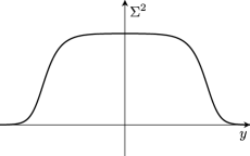
(a)		(b)

Figure 5: A plot of the profile $\Sigma^{2}$ of the domain wall with three Higgs flavors. The height of the function is suitably normalized to compare the profiles of different FI parameters with each other. (a) The shape is similar to the position-dependent coupling in §3 when $c_{1}/c_{2}\sim 1$. (b) We can also obtain the step-function like profile when $c_{1}/c_{2}\gg 1$.

5.3 Position-dependent coupling function from the cubic prepotential

Interactions between hypermultiplets and vector multiplets are specified by charge assignments of the hypermultiplets, whereas interactions among vector multiplets are specified by the so-called prepotential $a(\Sigma)$. It has been found from general principles[16] that the prepotential, which gives the Chern-Simons coupling for gauge fields together with other terms, in our five-dimensional theory should be at most cubic in vector multiplets. Let us write the bosonic part of a Lagrangian with the prepotential $a(\Sigma)$, by denoting the group label and gauge generators collectively as $I$. Each $U(1)$ factor group can have a triplet of the FI term with the parameters $c^{\alpha I}$ and the auxiliary fields $Y^{\alpha I}$, $\alpha=1,2,3$. Restoring two complex scalar $H^{irA},i=1,2$ for the hypermultiplets with the color ($G$) indices $r$ and the flavor indices $A$, we obtain

$${\cal L} = a_{IJ}\left(-{1\over 4}F_{MN}^{I}F^{JMN}+{1\over 2}D_{M}\Sigma^{I}D^{M}\Sigma^{J}+{1\over 2}Y^{\alpha I}Y^{\alpha J}\right)-c^{\alpha I}Y^{\alpha I}$$ (72)

$$+ a_{IJK}\left\{-{1\over 24}\epsilon^{LMNPQ}W_{L}^{I}\left(F^{J}_{MN}F^{K}_{PQ}+{1\over 2}[W_{M},W_{N}]^{J}F^{K}_{PQ}+{1\over 16}[W_{M},W_{N}]^{J}[W_{P},W_{Q}]^{K}\right)\right\}$$

$$+ ({\cal D}_{M}H^{irA})^{*}{\cal D}^{M}H^{irA}-(H^{irA})^{*}[(q^{I}\Sigma^{I}-m_{A})^{2}]^{r}{}_{s}H^{isA}$$

$$+ (H^{irA})^{*}(\sigma^{\alpha})^{i}{}_{j}q^{I}(Y^{\alpha I})^{r}{}_{s}H^{jsA},$$

where $m_{A}$ is the mass of the $A$-th hypermultiplet, and the derivative of prepotential $a(\Sigma)$ is denoted by subscripts like

$$a_{I}\equiv{\partial a(\Sigma)\over\partial\Sigma^{I}},\quad a_{IJ}\equiv{\partial^{2}a(\Sigma)\over\partial\Sigma^{I}\partial\Sigma^{J}},\quad a_{IJK}\equiv{\partial^{3}a(\Sigma)\over\partial\Sigma^{I}\partial\Sigma^{J}\partial\Sigma^{K}}.$$ (73)

Covariant derivatives ${\cal D}_{M}$ and $q^{I}\Sigma^{I}-m_{A}$ are understood to contain both $U(1)$ and non-Abelian components with appropriate charges or representation matrices. We note that the gauge field kinetic term multiplied by the scalar $\Sigma^{I}$ arises as a supersymmetric completion of the Chern-Simons term, both of which follow from the cubic prepotential.

The minimal kinetic term for $U(1)$ vector multiplets is represented by a term of the form $\Sigma^{I}\Sigma^{I}$ in the prepotential. As given in the previous subsections, the domain wall solution leads to a nontrivial kink profile for hypermultiplet scalars $H_{A}^{i}$, and the vector multiplet scalars $\Sigma^{I}$. Let us call those hypermultiplets and vector multiplets participating to form the domain wall as the domain wall sector. As described in §1, we wish to avoid the bulk in the Higgs phase in order to obtain localized gauge fields. This requirement is achieved by demanding the domain wall hypermultiplets to be neutral under the non-Abelian gauge fields which we wish to localize. Then the non-Abelian gauge fields can couple to the domain wall sector only through the prepotential among vector multiplets. Since the non-Abelian vector multiplets cannot appear linearly, the coupling between non-Abelian vector multiplets and domain wall sector should be linear in (a linear combination of) $U(1)$ vector multiplets in the domain wall sector. By choosing a linear combination $a_{1}\Sigma^{1}+a_{2}\Sigma^{2}$ of two $U(1)$ vector multiplets, we can obtain a desired profile of the position-dependent coupling function $\epsilon(y)$ at both infinities $y\to\pm\infty$, namely the asymptotically vanishing profile with a peak in the middle. Therefore we shall consider gauge group to be $U(1)\times U(1)\times G$ with $G$ as the non-Abelian gauge group which we wish to localize on the domain wall, and assume the following prepotential

$$a\left(\Sigma\right)={1\over 2e_{1}^{2}}(\Sigma^{1})^{2}+{1\over 2e_{2}^{2}}(\Sigma^{2})^{2}+{1\over 2}(a_{1}\Sigma^{1}+a_{2}\Sigma^{2})\Sigma^{a}\Sigma^{a}$$ (74)

whose constant coefficients $a_{1},a_{2}$ are chosen appropriately for each model of the domain wall sector. The first and second terms reproduce the minimal kinetic terms for the $U(1)$ vector multiplets, as we assumed in previous subsections.

Since the non-Abelian vector multiplet $\Sigma^{a}$ appear only quadratically in the prepotential because of gauge invariance, it is easy to see that the above prepotential allows the BPS domain wall solution in the previous sections to remain a solution to the entire system of field equations. Therefore we can safely choose the BPS domain wall solution as the background solution and consider the effective Lagrangian on the domain wall. If we choose the following coefficients of the prepotential, we obtain the position-dependent gauge coupling function $\epsilon(y)$ for the non-Abelian gauge fields. For the model with four matter fields in §4.2.1, we choose

$$a_{1}=-a_{2}\equiv a>0.$$ (75)

For the model with three matter fields in §4.2.2, we choose

$$a_{1}=0,\qquad a_{2}>0.$$ (76)

The value of the effective gauge coupling in four-dimensional world-volume in Eq.(4) can be adjusted by choosing the value of these coefficients $a$ or $a_{2}$.

6 Conclusion and Discussion

In this paper, we have discussed the localization of the massless vector fields by means of the position-dependent gauge coupling. We gave a few concrete examples where there exist the massless vector field and mass gap, and the Coulomb law emerges inside the domain wall. We expect that these localization properties do not depend on the details of the concrete coupling functions. If the position-dependent coupling function is everywhere nonnegative and vanishes at both infinities (weak coupling only at the center of the domain wall), the localization of the gauge field should occur in a similar way.

The position-dependent coupling function desired for the localization can be realized by the cubic prepotential of the five dimensional supersymmetric gauge theory. The coupling function comes about thanks to the profile of the domain walls of the Abelian subsectors. We expect that these coupling functions offer appropriate examples for the localization of non-Abelian gauge fields, although the explicit functional forms of the coupling functions in our concrete examples of domain wall are somewhat more involved than our solvable examples in §3.

In this paper, we considered the tree-level prepotential, in order to obtain the position-dependent coupling. The prepotential of the supersymmetric gauge theory with eight supercharges receives the nonperturbative quantum corrections generally. It is an interesting future problem to explore if our mechanism of localization of gauge fields due to the position-dependent coupling may be realized as a result of the nonperturbative quantum effects.

We have succeeded to localize non-Abelian gauge fields. However, we still need to introduce matter fields in nontrivial representations of the non-Abelian gauge group, in order to build the standard model localized on the domain wall. It has been found that a non-Abelian flavor symmetry for degenerate hypermultiplets provides non-Abelian orientational moduli for domain walls.[30] These orientational moduli arises in nontrivial representations of the non-Abelian flavor group. If we promote (a part of) the flavor symmetry to a local gauge symmetry, these non-Abelian orientational moduli fields become matter fields interacting nontrivially with the non-Abelian gauge fields. We can introduce matter fields coupled to the non-Abelian gauge fields of our model in this way. In order to construct the standard model localized on the domain wall, it remains to see if matter fields in appropriate (chiral) representations can be introduced into our framework. The interaction of localized matter fields and the localized gauge fields offers an intriguing question of charge universality [33]. Our model should provide a concrete example of localized matter fields assuring the charge universality.

We have succeeded to embed the BPS domain wall solutions in flat space into the five-dimensional supergravity theory, and found a model with the warped extra dimension.[31, 32] It is also an interesting future problem to embed our mechanism of localized gauge fields into supergravity. In this context, it is worthwhile to examine a recent objection against the Fayet-Iliopoulos parameter in supergravity.[34]

Appendix A Threshold bound states and wave functions

In this Appendix, we consider an eigenvalue problem of the following static Schrödinger equation discussed in §3

$$\left[-\frac{1}{2}\frac{d^{2}}{dY^{2}}+U(Y)\right]\psi(Y)=E\psi(Y)\quad\text{for}\quad-\infty<Y<\infty.$$ (77)

We will find wave functions of the threshold bound states satisfying $E=0$ by choosing a suitable height of the potential $U(Y)$.

A.1 cosh potential

Let us first take the potential $U(Y)=-U_{0}/\cosh^{2}\alpha Y$ in Eq.(24) (see Fig.1). Changing the variable by $\xi=\tanh\alpha Y$ ($-1<\xi<1$) and defining $2U_{0}/\alpha^{2}=s(s+1)$, and ${\cal E}\equiv\sqrt{-2E}/\alpha$, (77) becomes

$$\left[\frac{d}{d\xi}(1-\xi^{2})\frac{d}{d\xi}+s(s+1)-\frac{{\cal E}}{1-\xi^{2}}\right]\psi(\xi)=0.$$ (78)

In order to find a series solution around $\xi=1$, we define $u=(1-\xi)/2$ and assume $\psi=u^{\gamma}\phi(u)=\sum_{l=0}^{\infty}a_{l}u^{l}$. By requiring a regular solution at $\xi=1$, we find $\gamma={\cal E}/{2}$. Using $\phi(u)$ instead of $\psi$, Eq.(78) reduces to

$$\left[u(1-u)\frac{d^{2}}{du^{2}}+{1+{\cal E}}(1-2u)\frac{d}{du}-({\cal E}-s)({\cal E}+s+1)\right]\phi(u)=0,$$ (79)

where $\phi(u)\equiv\sum_{l=0}^{\infty}a_{l}u^{l}$. In order to obtain solutions regular at $u=1$ ($\xi=-1$), the series in $\phi(u)=\sum_{l}a_{l}u^{l}$ has to terminate and ${\cal E}=s-n$. Thus the $n$-th eigenfunction is given by the following $n$-th order polynomial $\phi_{n}(u)$ with $0\leq n<s$ for a given $s$

$$\phi_{n}(u)=a_{0}\sum_{l=0}^{n}\frac{1}{l!}\frac{(l+2s-n)!}{(2s-n)!}\frac{n!}{(n-l)!}\frac{(s-n)!}{(l+s-n)!}(-u)^{l}.$$

Threshold bound state is given by ${\cal E}=0$, that is, $s=n$, which is achieved by choosing the potential height $U_{0}=\alpha^{2}n(n+1)/2$ as in Eq.(28). The wave function of the $n$-th threshold bound state is given by

$$\phi_{n}(u)=a_{0}\sum_{l=0}^{n}\frac{1}{(l!)^{2}}\frac{(n+l)!}{(n-l)!}(-u)^{l}.$$ (80)

A.2 square well potential

Here we consider the square well potential with a finite potential step in Eq.(31) (see Fig.2). The reflection symmetry $Y\to-Y$ dictates that eigenfunctions must be either an even or odd function. For $|Y|<a$, we obtain the eigenfunctions $\psi(Y)=A\cos kY$ for even functions, and $B\sin kY$ for odd functions, with $k=\sqrt{2(E+U_{0})}$. For $Y>a$, the boundary condition at infinity requires that $\psi(Y)=Ce^{-\beta|Y|}$ with $\beta=\sqrt{-2E}$. The bound state exists if and only if $E<0$. The connection condition at $Y=a$ gives $k\tan ka=\beta$ for even functions and $k\cot ka=-\beta$ for odd functions.

The threshold bound state with $E=0$ means that $\beta=0$, that is, the wave function becomes a constant outside of the well. The connection condition for $\beta=0$ is solved by discrete values of $k$: $k_{n}=\frac{n\pi}{2a}$ with nonnegative integer $n$, where $n$ is even for the even wave function and odd for the odd wave function, respectively. We obtain the $n$-th threshold bound state by choosing the potential depth $U_{0}=k^{2}/2={n^{2}\pi^{2}}/({8a^{2}})$ as in Eq.(32). The wave function of the $n$-th threshold bound state is given for even $n=2l$ ($l=0,1,2,\ldots$)

$$\psi_{n}(Y)=\left\{\begin{array}[]{ll}A\cos k_{n}Y&|Y|<a\\ A(-1)^{\frac{n}{2}}&|Y|>a\end{array}\right.,$$ (81)

and for odd $n=2l+1$ ($l=0,1,2,\ldots$)

$$\psi_{n}(Y)=\left\{\begin{array}[]{ll}B\sin k_{n}Y&|Y|<a\\ B(-1)^{\frac{n-1}{2}}&|Y|>a\end{array}\right..$$ (82)

References

-
[1]
S. Dimopoulos and H. Georgi,
Nucl. Phys. B 193 (1981) 150.
N. Sakai, Z. Phys. C 11 (1981) 153.
E. Witten, Nucl. Phys. B 188 (1981) 513. - [2] P. Horava and E. Witten, Nucl. Phys. B 460 (1996) 506 [arXiv:hep-th/9510209].
-
[3]
N. Arkani-Hamed, S. Dimopoulos and G. R. Dvali,
Phys. Lett. B 429 (1998) 263
[arXiv:hep-ph/9803315].
I. Antoniadis, N. Arkani-Hamed, S. Dimopoulos and G. R. Dvali, Phys. Lett. B 436 (1998) 257 [arXiv:hep-ph/9804398]. - [4] L. Randall and R. Sundrum, Phys. Rev. Lett. 83 (1999) 3370 [arXiv:hep-ph/9905221];Phys. Rev. Lett. 83 (1999) 4690 [arXiv:hep-th/9906064].
- [5] H. Davoudiasl, J. L. Hewett and T. G. Rizzo, Phys. Lett. B 473 (2000) 43 [arXiv:hep-ph/9911262].
- [6] A. Pomarol, Phys. Lett. B 486 (2000) 153 [arXiv:hep-ph/9911294].
- [7] B. Batell and T. Gherghetta, Phys. Rev. D 73 (2006) 045016 [arXiv:hep-ph/0512356]; Phys. Rev. D 75 (2007) 025022 [arXiv:hep-th/0611305].
- [8] Y. Isozumi, K. Ohashi and N. Sakai, JHEP 0311 (2003) 061 [arXiv:hep-th/0310130].
- [9] G. R. Dvali and M. A. Shifman, Phys. Lett. B 396 (1997) 64 [Erratum-ibid. B 407 (1997) 452] [arXiv:hep-th/9612128].
-
[10]
M. Shifman and A. Yung,
Phys. Rev. D 67 (2003) 125007
[arXiv:hep-th/0212293]; Phys. Rev. D 70 (2004) 025013
[arXiv:hep-th/0312257].
R. Auzzi, S. Bolognesi, M. Shifman and A. Yung, Phys. Rev. D 79 (2009) 045016 [arXiv:0807.1908 [hep-th]]. - [11] S. L. Dubovsky and V. A. Rubakov, Int. J. Mod. Phys. A 16 (2001) 4331 [arXiv:hep-th/0105243].
- [12] N. Maru and N. Sakai, Prog. Theor. Phys. 111 (2004) 907 [arXiv:hep-th/0305222].
-
[13]
Y. K. Fu and H. B. Nielsen,
Nucl. Phys. B 236 (1984) 167; Nucl. Phys. B 254 (1985) 127.
P. Dimopoulos, K. Farakos, A. Kehagias and G. Koutsoumbas, Nucl. Phys. B 617 (2001) 237 [arXiv:hep-th/0007079]. - [14] J. B. Kogut and L. Susskind, Phys. Rev. D 9 (1974) 3501.
- [15] R. Fukuda, Phys. Lett. B 73 (1978) 305 [Erratum-ibid. B 74 (1978) 433];Mod. Phys. Lett. A 24 (2009) 251;arXiv:0805.3864 [hep-th].
-
[16]
N. Seiberg,
Phys. Lett. B 388 (1996) 753
[arXiv:hep-th/9608111].
D. R. Morrison and N. Seiberg, Nucl. Phys. B 483 (1997) 229 [arXiv:hep-th/9609070]. - [17] L. D. Landau and L. M. Lifshitz, “Quantum Mechanics (Non-Relativistic Theory),” Butterworth-Heinemann (1981).
- [18] G. R. Dvali, G. Gabadadze and M. A. Shifman, Phys. Lett. B 497 (2001) 271 [arXiv:hep-th/0010071].
- [19] J. P. Gauntlett, D. Tong and P. K. Townsend, Phys. Rev. D 64 (2001) 025010 [arXiv:hep-th/0012178].
- [20] D. Tong, Phys. Rev. D 66 (2002) 025013 [arXiv:hep-th/0202012].
- [21] J. P. Gauntlett, D. Tong and P. K. Townsend, Phys. Rev. D 63 (2001) 085001 [arXiv:hep-th/0007124].
- [22] M. Arai, M. Naganuma, M. Nitta and N. Sakai, Nucl. Phys. B 652 (2003) 35 [arXiv:hep-th/0211103].
- [23] Y. Isozumi, K. Ohashi and N. Sakai, JHEP 0311 (2003) 060 [arXiv:hep-th/0310189].
- [24] Y. Isozumi, M. Nitta, K. Ohashi and N. Sakai, Phys. Rev. Lett. 93 (2004) 161601 [arXiv:hep-th/0404198].
- [25] Y. Isozumi, M. Nitta, K. Ohashi and N. Sakai, Phys. Rev. D 70 (2004) 125014 [arXiv:hep-th/0405194].
- [26] M. Eto, Y. Isozumi, M. Nitta, K. Ohashi, K. Ohta and N. Sakai, Phys. Rev. D 71 (2005) 125006 [arXiv:hep-th/0412024].
- [27] M. Eto, Y. Isozumi, M. Nitta, K. Ohashi, K. Ohta, N. Sakai and Y. Tachikawa, Phys. Rev. D 71 (2005) 105009 [arXiv:hep-th/0503033].
- [28] N. Sakai and Y. Yang, Commun. Math. Phys. 267 (2006) 783 [arXiv:hep-th/0505136].
- [29] M. Eto, Y. Isozumi, M. Nitta, K. Ohashi and N. Sakai, J. Phys. A 39 (2006) R315 [arXiv:hep-th/0602170].
- [30] M. Eto, T. Fujimori, M. Nitta, K. Ohashi and N. Sakai, Phys. Rev. D 77 (2008) 125008 [arXiv:0802.3135 [hep-th]], “Domain walls with non-Abelian orientational moduli,” arXiv:0912.3590 [hep-th].
- [31] M. Arai, S. Fujita, M. Naganuma and N. Sakai, Phys. Lett. B 556 (2003) 192 [arXiv:hep-th/0212175].
- [32] M. Eto, S. Fujita, M. Naganuma and N. Sakai, Phys. Rev. D 69 (2004) 025007 [arXiv:hep-th/0306198].
- [33] S. L. Dubovsky, V. A. Rubakov and P. G. Tinyakov, JHEP 0008 (2000) 041 [arXiv:hep-ph/0007179].
- [34] Z. Komargodski and N. Seiberg, JHEP 0906 (2009) 007 [arXiv:0904.1159 [hep-th]].