Eagle Strategy Using Lévy Walk and Firefly Algorithms For Stochastic Optimization

Abstract

Most global optimization problems are nonlinear and thus difficult to solve, and they become even more challenging when uncertainties are present in objective functions and constraints. This paper provides a new two-stage hybrid search method, called Eagle Strategy, for stochastic optimization. This strategy intends to combine the random search using Lévy walk with the firefly algorithm in an iterative manner. Numerical studies and results suggest that the proposed Eagle Strategy is very efficient for stochastic optimization. Finally practical implications and potential topics for further research will be discussed.

Citation detail:

X.-S. Yang and S. Deb, Eagle strategy using Levy walk and firefly algorithms for stochastic optimization, in: Nature Inspired Cooperative Strategies for Optimization (NISCO 2010) (Eds. J. R. Gonzalez et al., Studies in Computational Intelligence, Springer Berlin, 284, 101-111 (2010).

1 Introduction

To find the solutions to any optimization problems, we can use either conventional optimization algorithms such as the Hill-climbing and simplex method, or heuristic methods such as genetic algorithms, or their proper combinations. Modern metaheuristic algorithms are becoming powerful in solving global optimization problems [4, 6, 7, 9, 20, 21, 22], especially for the NP-hard problems such as the travelling salesman problem. For example, particle swarm optimization (PSO) was developed by Kennedy and Eberhart in 1995 [8, 9], based on the swarm behaviour such as fish and bird schooling in nature. It has now been applied to find solutions for many optimization applications. Another example is the Firefly Algorithm developed by the first author [20, 21] which has demonstrated promising superiority over many other algorithms. The search strategies in these multi-agent algorithms are controlled randomization and exploitation of the best solutions. However, such randomization typically uses a uniform distribution or Gaussian distribution. In fact, since the development of PSO, quite a few algorithms have been developed and they can outperform PSO in different ways [21, 23].

On the other hand, there is always some uncertainty and noise associated with all real-world optimization problems. Subsequently, objective functions may have noise and constraints may also have random noise. In this case, a standard optimization problem becomes a stochastic optimization problem. Methods that work well for standard optimization problems cannot directly be applied to stochastic optimization; otherwise, the obtained results are incorrect or even meaningless. Either the optimization problems have to be reformulated properly or the optimization algorithms should be modified accordingly, though in most cases we have to do both [3, 10, 19]

In this paper, we intend to formulate a new metaheuristic search method, called Eagle Stategy (ES), which combines the Lévy walk search with the Firefly Algorithm (FA). We will provide the comparison study of the ES with PSO and other relevant algorithms. We will first outline the basic ideas of the Eagle Strategy, then outline the essence of the firefly algorithm, and finally carry out the comparison about the performance of these algorithms.

2 Stochastic Multiobjective Optimization

An ordinary optimization problem, without noise or uncertainty, can be written as

$$\min_{{\bf x}\in\Re^{d}}f_{i}({\bf x}),\;(i=1,2,...,N)$$ (1)

$$\textrm{subject to }\phi_{j}({\bf x})=0,\;(j=1,2,...,J),$$

$$\qquad\qquad\psi_{k}({\bf x})\leq 0,\;(k=1,2,...,K),$$ (2)

where ${\bf x}=(x_{1},x_{2},...,x_{d})^{T}$ is the vector of design variables.

For stochastic optimization problems, the effect of uncertainty or noise on the design variable $x_{i}$ can be described by a random variable $\xi_{i}$ with a distribution $Q_{i}$ [10, 19]. That is

$$x_{i}\mapsto\xi_{i}(x_{i}),$$ (3)

and

$$\xi_{i}\sim Q_{i}.$$ (4)

The most widely used distribution is the Gaussian or normal distribution $N(x_{i},\sigma_{i})$ with a mean $x_{i}$ and a known standard deviation $\sigma_{i}$. Consequently, the objective functions $f_{i}$ become random variables $f_{i}({\bf x},\xi)$.

Now we have to reformulate the optimization problem as the minimization of the mean of the objective function $f_{i}({\bf x})$ or $\mu_{f_{i}}$

$$\min_{{\bf x}\in\Re^{d}}\{\mu_{f_{1}},...,\mu_{f_{N}}\}.$$ (5)

Here $\mu_{f_{i}}=E(f_{i})$ is the mean or expectation of $f_{i}(\xi({\bf x}))$ where $i=1,2,...,N$. More generally, we can also include their uncertainties, which leads to the minimization of

$$\min_{{\bf x}\in\Re^{d}}\{\mu_{f_{1}}+\lambda\sigma_{1},...,\mu_{f_{N}}+\lambda\sigma_{N}\},$$ (6)

where $\lambda\geq 0$ is a constant. In addition, the constraints with uncertainty should be modified accordingly.

In order to estimate $\mu_{f_{i}}$, we have to use some sampling techniques such as the Monte Carlo method. Once we have randomly drawn the samples, we have

$$\mu_{f_{i}}\approx\frac{1}{N_{i}}\sum_{p=1}^{N_{i}}f_{i}({\bf x},\xi^{(p)}),$$ (7)

where $N_{i}$ is the number of samples.

3 Eagle Strategy

The foraging behaviour of eagles such as golden eagles or Aquila Chrysaetos is inspiring. An eagle forages in its own territory by flying freely in a random manner much like the Lévy flights. Once the prey is sighted, the eagle will change its search strategy to an intensive chasing tactics so as to catch the prey as efficiently as possible. There are two important components to an eagle’s hunting strategy: random search by Lévy flight (or walk) and intensive chase by locking its aim on the target.

Furthermore, various studies have shown that flight behaviour of many animals and insects has demonstrated the typical characteristics of Lévy flights [5, 14, 12, 13]. A recent study by Reynolds and Frye shows that fruit flies or Drosophila melanogaster, explore their landscape using a series of straight flight paths punctuated by a sudden $90^{0}$ turn, leading to a Lévy-flight-style intermittent scale-free search pattern. Studies on human behaviour such as the Ju/’hoansi hunter-gatherer foraging patterns also show the typical feature of Lévy flights. Even light can be related to Lévy flights [2]. Subsequently, such behaviour has been applied to optimization and optimal search, and preliminary results show its promising capability [12, 14, 16, 17].

3.1 Eagle Strategy

Now let us idealize the two-stage strategy of an eagle’s foraging behaviour. Firstly, we assume that an eagle will perform the Lévy walk in the whole domain. Once it finds a prey it changes to a chase strategy. Secondly, the chase strategy can be considered as an intensive local search using any optimization technique such as the steepest descent method, or the downhill simplex or Nelder-Mead method [11]. Obviously, we can also use any efficient metaheuristic algorithms such as the particle swarm optimization (PSO) and the Firefly Algorithm (FA) to do concentrated local search. The pseudo code of the proposed eagle strategy is outlined in Fig. 1.

The size of the hypersphere depends on the landscape of the objective functions. If the objective functions are unimodal, then the size of the hypersphere can be about the same size of the domain. The global optimum can in principle be found from any initial guess. If the objective are multimodal, then the size of the hypersphere should be the typical size of the local modes. In reality, we do not know much about the landscape of the objective functions before we do the optimization, and we can either start from a larger domain and shrink it down or use a smaller size and then gradually expand it.

On the surface, the eagle strategy has some similarity with the random-restart hill climbing method, but there are two important differences. Firstly, ES is a two-stage strategy rather than a simple iterative method, and thus ES intends to combine a good randomization (diversification) technique of global search with an intensive and efficient local search method. Secondly, ES uses Lévy walk rather than simple randomization, which means that the global search space can be explored more efficiently. In fact, studies show that Lévy walk is far more efficient than simple random-walk exploration.

Eagle Strategy   Objective functions $f_{1}({\bf x}),...,f_{N}({\bf x})$
 Initial guess ${\bf x}^{t=0}$
 while ($||{\bf x}^{t+1}-{\bf x}^{t}||>$ tolerance)
 Random search by performing Lévy walk
 Evaluate the objective functions
 Intensive local search with a hypersphere
   via Nelder-Mead or the Firefly Algorithm
  if (a better solution is found)
   Update the current best
  end if
  Update $t=t+1$
  Calculate means and standard deviations
 end while
Postprocess results and visualization  

Figure 1: Pseudo code of the Eagle Strategy (ES).

The Lévy walk has a random step length being drawn from a Lévy distribution

$$\textrm{L\'{e}vy}\sim u=t^{-\lambda},\quad(1<\lambda\leq 3),$$ (8)

which has an infinite variance with an infinite mean. Here the steps of the eagle motion is essentially a random walk process with a power-law step-length distribution with a heavy tail. The special case $\lambda=3$ corresponds to Brownian motion, while $\lambda=1$ has a characteristics of stochastic tunneling, which may be more efficient in avoiding being trapped in local optima.

For the local search, we can use any efficient optimization algorithm such as the downhill simplex (Nelder-Mead) or metaheuristic algorithms such as PSO and the firefly algorithm. In this paper, we used the firefly algorithm to do the local search, since the firefly algorithm was designed to solve multimodal global optimization problems [21].

3.2 Firefly Algorithm

We now briefly outline the main components of the Firefly Algorithm developed by the first author [20], inspired by the flash pattern and characteristics of fireflies. For simplicity in describing the algorithm, we now use the following three idealized rules: 1) all fireflies are unisex so that one firefly will be attracted to other fireflies regardless of their sex; 2) Attractiveness is proportional to their brightness, thus for any two flashing fireflies, the less brighter one will move towards the brighter one. The attractiveness is proportional to the brightness and they both decrease as their distance increases. If there is no brighter one than a particular firefly, it will move randomly; 3) The brightness of a firefly is affected or determined by the landscape of the objective function. For a maximization problem, the brightness can simply be proportional to the value of the objective functions.

Firefly Algorithm   Objective function $f_{p}({\bf x}),\;{\bf x}=(x_{1},...,x_{d})^{T}$
Initial population of fireflies ${\bf x}_{i}\;(i=1,...,n)$
Light intensity $I_{i}$ at ${\bf x}_{i}$ is determined by $f_{p}({\bf x}_{i})$
Define light absorption coefficient $\gamma$
while ($t<$MaxGeneration)
 for $i=1:n$ all $n$ fireflies
  for $j=1:i$ all $n$ fireflies
  if ($I_{j}>I_{i}$)
    Move firefly $i$ towards $j$ ($d$-dimension)
  end if
  Vary $\beta$ via $\exp[-\gamma r]$
  Evaluate new solutions and update
  end for $j$
 end for $i$
Rank the fireflies and find the current best
end while
Postprocess results and visualization  

Figure 2: Pseudo code of the firefly algorithm (FA).

In the firefly algorithm, there are two important issues: the variation of light intensity and formulation of the attractiveness. For simplicity, we can always assume that the attractiveness of a firefly is determined by its brightness which in turn is associated with the encoded objective function.

In the simplest case for maximum optimization problems, the brightness $I$ of a firefly at a particular location ${\bf x}$ can be chosen as $I({\bf x})\propto f({\bf x})$. However, the attractiveness $\beta$ is relative, it should be seen in the eyes of the beholder or judged by the other fireflies. Thus, it will vary with the distance $r_{ij}$ between firefly $i$ and firefly $j$. In addition, light intensity decreases with the distance from its source, and light is also absorbed in the media, so we should allow the attractiveness to vary with the degree of absorption. In the simplest form, the light intensity $I(r)$ varies according to the inverse square law $I(r)=\frac{I_{s}}{r^{2}}$ where $I_{s}$ is the intensity at the source. For a given medium with a fixed light absorption coefficient $\gamma$, the light intensity $I$ varies with the distance $r$. That is

$$I=I_{0}e^{-\gamma r},$$ (9)

where $I_{0}$ is the original light intensity.

As a firefly’s attractiveness is proportional to the light intensity seen by adjacent fireflies, we can now define the attractiveness $\beta$ of a firefly by

$$\beta=\beta_{0}e^{-\gamma r^{2}},$$ (10)

where $\beta_{0}$ is the attractiveness at $r=0$.

The distance between any two fireflies $i$ and $j$ at ${\bf x}_{i}$ and ${\bf x}_{j}$, respectively, is the Cartesian distance

$$r_{ij}=||{\bf x}_{i}-{\bf x}_{j}||=\sqrt{\sum_{k=1}^{d}(x_{i,k}-x_{j,k})^{2}},$$ (11)

where $x_{i,k}$ is the $k$th component of the spatial coordinate ${\bf x}_{i}$ of $i$th firefly. In the 2-D case, we have

$$r_{ij}=\sqrt{(x_{i}-x_{j})^{2}+(y_{i}-y_{j})^{2}}.$$ (12)

The movement of a firefly $i$ is attracted to another more attractive (brighter) firefly $j$ is determined by

$${\bf x}_{i}={\bf x}_{i}+\beta_{0}e^{-\gamma r^{2}_{ij}}({\bf x}_{j}-{\bf x}_{i})+\alpha\;({\rm rand}-\frac{1}{2}),$$ (13)

where the second term is due to the attraction. The third term is randomization with a control parameter $\alpha$, which makes the exploration of the search space more efficient.

We have tried to use different values of the parameters $\alpha,\beta_{0},\gamma$ [20, 21], after some simulations, we concluded that we can use $\beta_{0}=1$, $\alpha\in[0,1]$, $\gamma=1$, and $\lambda=1$ for most applications. In addition, if the scales vary significantly in different dimensions such as $-10^{5}$ to $10^{5}$ in one dimension while, say, $-0.001$ to $0.01$ along the other, it is a good idea to replace $\alpha$ by $\alpha S_{k}$ where the scaling parameters $S_{k}(k=1,...,d)$ in the $d$ dimensions should be determined by the actual scales of the problem of interest.

There are two important limiting cases when $\gamma\rightarrow 0$ and $\gamma\rightarrow\infty$. For $\gamma\rightarrow 0$, the attractiveness is constant $\beta=\beta_{0}$ and the length scale $\Gamma=1/\sqrt{\gamma}\rightarrow\infty$, this is equivalent to say that the light intensity does not decrease in an idealized sky. Thus, a flashing firefly can be seen anywhere in the domain. Thus, a single (usually global) optimum can easily be reached. This corresponds to a special case of particle swarm optimization (PSO) discussed earlier. Subsequently, the efficiency of this special case could be about the same as that of PSO.

On the other hand, the limiting case $\gamma\rightarrow\infty$ leads to $\Gamma\rightarrow 0$ and $\beta(r)\rightarrow\delta(r)$ (the Dirac delta function), which means that the attractiveness is almost zero in the sight of other fireflies or the fireflies are short-sighted. This is equivalent to the case where the fireflies roam in a very foggy region randomly. No other fireflies can be seen, and each firefly roams in a completely random way. Therefore, this corresponds to the completely random search method. As the firefly algorithm is usually in somewhere between these two extremes, it is possible to adjust the parameter $\gamma$ and $\alpha$ so that it can outperform both the random search and PSO.

4 Simulations and Comparison

4.1 Validation

In order to validate the proposed algorithm, we have implemented it in Matlab. In our simulations, the values of the parameters are $\alpha=0.2$, $\gamma=1$, $\lambda=1$, and $\beta_{0}=1$.

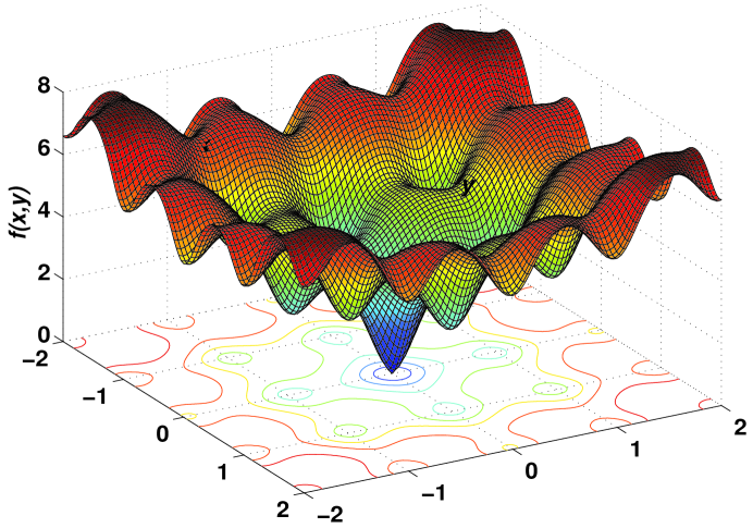
Figure 3: Ackley’s function for two independent variables with a global minimum $f_{*}=0$ at $(0,0)$.

As an example, we now use the ES to find the global optimum of the Ackley function

$$f({\bf x})=-20\exp[-\frac{1}{5}\sqrt{\frac{1}{d}\sum_{i=1}^{d}x_{i}^{2}}]-\exp[\frac{1}{d}\sum_{i=1}^{d}\cos(2\pi x_{i})]+20+e,$$ (14)

where $(d=1,2,...)$ [1]. The global minimum $f_{*}=0$ occurs at $(0,0,...,0)$ in the domain of $-32.768\leq x_{i}\leq 32.768$ where $i=1,2,...,d$. The landscape of the 2D Ackley function is shown in Fig. 3, while the landscape of this function with $2.5\%$ noise is shown in Fig. 4

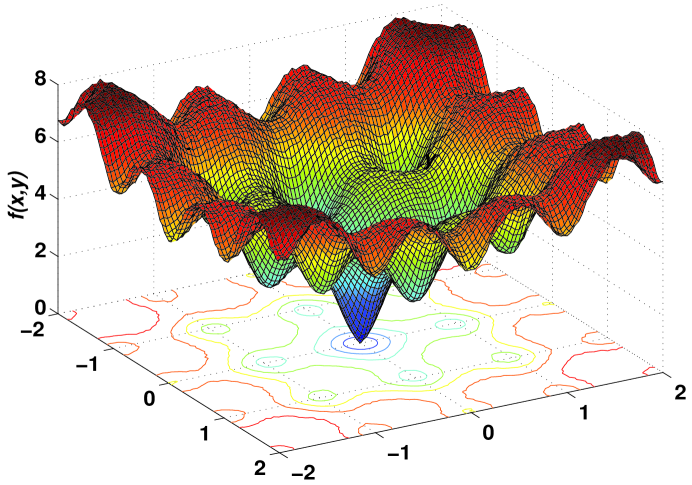
Figure 4: Ackley’s 2D function with Gaussian noise.

The global minimum in 2D for a given noise level of $2.5\%$ can be found after about 300 function evaluations (for 20 fireflies after 15 iterations, see Fig. 5).

4.2 Comparison of ES with PSO

Various studies show that PSO algorithms can outperform genetic algorithms (GA) [7] and other conventional algorithms for solving many optimization problems. This is partially due to that fact that the broadcasting ability of the current best estimates gives better and quicker convergence towards the optimality. A general framework for evaluating statistical performance of evolutionary algorithms has been discussed in detail by Shilane et al. [15].

Now we will compare the Eagle Strategy with PSO for various standard test functions. After implementing these algorithms using Matlab, we have carried out extensive simulations and each algorithm has been run at least 100 times so as to carry out meaningful statistical analysis. The algorithms stop when the variations of function values are less than a given tolerance $\epsilon\leq 10^{-5}$. The results are summarized in the following table (see Table 1) where the global optima are reached. The numbers are in the format: average number of evaluations (success rate), so $12.7\pm 1.15(100)$ means that the average number (mean) of function evaluations is $12.7\times 10^{3}=12700$ with a standard deviation of $1.15\times 10^{3}=1150$. The success rate of finding the global optima for this algorithm is $100\%$. Here we have used the following abbreviations: MWZ for Michalewicz’s function with $d=16$, RBK for Rosenbrock with $d=16$, De Jong for De Jong’s sphere function with $d=256$, Schwefel for Schwefel with $d=128$, Ackley for Ackley’s function with $d=128$, and Shubert for Shubert’s function with 18 minima. In addition, all these test functions have a $2.5\%$ of Gaussian noise, or $\sigma=0.025$. In addition, we have used the population size $n=20$ in all our simulations.

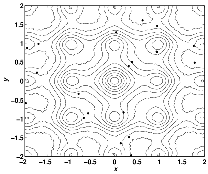
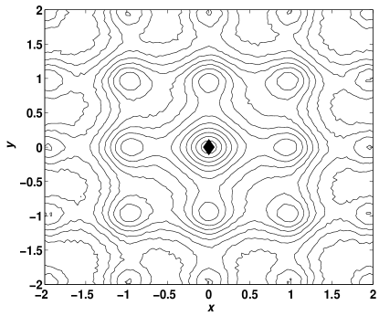
Figure 5: The initial locations of the 20 fireflies (left) and their locations after $15$ iterations (right). We have used $\gamma=1$.

Table 1: Comparison of algorithm performance

	PSO ($\times 10^{3}$)	ES ($\times 10^{3}$)
Easom	$185.9\pm 3.1(97)$	$12.7\pm 1.15(100)$
MWZ	$346.1\pm 8.0(98)$	$36.1\pm 3.5(100)$
Rosenbrock	$1637\pm 79(98)$	$75\pm 6.4(100)$
De Jong	$852\pm 16(100)$	$70.7\pm 7.3(100)$
Schwefel	$726.1\pm 25(97)$	$99\pm 6.7(100)$
Ackley	$1170\pm 19(92)$	$54\pm 5.2(100)$
Rastrigin	$3973\pm 64(90)$	$151\pm 14(100)$
Easom	$863.7\pm 55(90)$	$76\pm 11(100)$
Griewank	$2798\pm 63(92)$	$134\pm 9.1(100)$
Shubert	$1197\pm 56(92)$	$32\pm 2.5(100)$

We can see that the ES is noticeably more efficient in finding the global optima with the success rates of $100\%$. Each function evaluation is virtually instantaneous on a modern personal computer. For example, the computing time for 10,000 evaluations on a 3GHz desktop is about 5 seconds. Even with graphics for displaying the locations of the particles and fireflies, it usually takes less than a few minutes. Furthermore, we have used various values of the population size $n$ or the number of fireflies. We found that for most problems $n=15$ to $50$ would be sufficient. For tougher problems, larger $n$ such as $n=100$ or $250$ can be used, though excessively large $n$ should not be used unless there is no better alternative, as it is more computationally extensive.

5 Conclusions

By combining Lévy walk with the firefly algorithm, we have successfully formulated a hybrid optimization algorithm, called Eagle Strategy, for stochastic optimization. After briefly outlining the basic procedure and its similarities and differences with particle swarm optimization, we then implemented and compared these algorithms. Our simulation results for finding the global optima of various test functions suggest that ES can significantly outperform the PSO in terms of both efficiency and success rate. This implies that ES is potentially more powerful in solving NP-hard problems.

However, we have not carried out sensitivity studies of the algorithm-dependent parameters such as the exponent $\lambda$ in Lévy distribution and the light absorption coefficient $\gamma$, which may be fine-tuned to a specific problem. This can form an important research topic for further research. Furthermore, other local search algorithms such as the Newton-Raphson method, sequential quadratic programming and Nelder-Mead algorithms can be used to replace the firefly algorithm, and a comparison study should be carried out to evaluate their performance. It may also show interesting results if the level of uncertainty varies and it can be expected that the higher level of noise will make it more difficult to reach optimal solutions.

As other important further studies, we can also focus on the applications of this hybrid algorithm on the NP-hard traveling salesman problem. In addition, many engineering design problems typically have to deal with intrinsic inhomogeneous materials properties and such uncertainty may often affect the design choice in practice. The application of the proposed hybrid algorithm in engineering design optimization may prove fruitful.

References

- [1] Ackley, D. H.: A connectionist machine for genetic hillclimbing. Kluwer Academic Publishers, (1987).
- [2] Barthelemy, P., Bertolotti, J., Wiersma, D. S.: A Lévy flight for light. Nature, 453, 495-498 (2008).
- [3] Bental, A., El Ghaoui, L., Nemirovski, A.: Robust Optimization. Princeton University Press, (2009).
- [4] Bonabeau, E., Dorigo, M., Theraulaz, G.: Swarm Intelligence: From Natural to Artificial Systems. Oxford University Press, (1999)
- [5] Brown, C., Liebovitch, L. S., Glendon, R.: Lévy flights in Dobe Ju/’hoansi foraging patterns. Human Ecol., 35, 129-138 (2007).
- [6] Deb, K.: Optimisation for Engineering Design. Prentice-Hall, New Delhi, (1995).
- [7] Goldberg, D. E.: Genetic Algorithms in Search, Optimisation and Machine Learning. Reading, Mass.: Addison Wesley (1989).
- [8] Kennedy, J. and Eberhart, R. C.: Particle swarm optimization. Proc. of IEEE International Conference on Neural Networks, Piscataway, NJ. pp. 1942-1948 (1995).
- [9] Kennedy J., Eberhart R., Shi Y.: Swarm intelligence. Academic Press, (2001).
- [10] Marti, K.: Stochastic Optimization Methods. Springer, (2005).
- [11] Nelder, J. A. and Mead, R.: A simplex method for function minimization. Computer Journal, 7, 308-313 (1965).
- [12] Pavlyukevich, I.: Lévy flights, non-local search and simulated annealing. J. Computational Physics, 226, 1830-1844 (2007).
- [13] Pavlyukevich, I.: Cooling down Lévy flights, J. Phys. A:Math. Theor., 40, 12299-12313 (2007).
- [14] Reynolds, A. M. and Frye, M. A.: Free-flight odor tracking in Drosophila is consistent with an optimal intermittent scale-free search. PLoS One, 2, e354 (2007).
- [15] Shilane, D., Martikainen, J., Dudoit, S., Ovaska S. J.: A general framework for statistical performance comparison of evolutionary computation algorithms. Information Sciences: an Int. Journal, 178, 2870-2879 (2008).
- [16] Shlesinger, M. F., Zaslavsky, G. M. and Frisch, U. (Eds): Lévy Flights and Related Topics in Phyics. Springer, (1995).
- [17] Shlesinger, M. F.: Search research. Nature, 443, 281-282 (2006).
- [18] Urfalioglu, O., Cetin, A. E., Kuruoglu, E. E.: Levy walk evolution for global optimization. in: Proc. of 10th Genetic and Evolutionary Computation Conference, pp.537-538 (2008).
- [19] Wallace, S. W., Ziemba, W. T.: Applications of Stochastic Programming. SIAM Mathematical Series on Optimization, (2005).
- [20] Yang X. S.: Nature-Inspired Metaheuristic Algorithms, Luniver Press, (2008).
- [21] Yang X. S.: Firefly algorithms for multimodal optimization. in: Stochastic Algorithms: Foundations and Applications (Eds. O. Watanabe and T. Zeugmann), Springer, SAGA 2009, Lecture Notes in Computer Science, 5792, 169-178 (2009).
- [22] Yang X. S. and Deb, S.: Cuckoo search via Lévy flights. Proceedings of World Congress on Nature & Biologically Inspired Computing (NaBic 2009), IEEE Pulications, India, 210-214(2009).
- [23] Yang, Z. Y., Tang, K., and Yao, X.: Large Scale Evolutionary Optimization Using Cooperative Coevolution. Information Sciences, 178, 2985-2999 (2008).