Optimal Liquidation Strategies Regularize Portfolio Selection

Abstract

We consider the problem of portfolio optimization in the presence of market impact, and derive optimal liquidation strategies. We discuss in detail the problem of finding the optimal portfolio under Expected Shortfall (ES) in the case of linear market impact. We show that, once market impact is taken into account, a regularized version of the usual optimization problem naturally emerges. We characterize the typical behavior of the optimal liquidation strategies, in the limit of large portfolio sizes, and show how the market impact removes the instability of ES in this context.

1 Introduction

The optimization of large portfolios is known to be highly unstable, due to large sample to sample fluctuations. This instability arises from the fact that risk measures need to be estimated from empirical observations in the market and for large portfolios we can never have enough data: by the very nature of portfolio selection, the sampling frequency cannot be high, and the look-back period cannot be too long. Therefore, the length $T$ of the available time series cannot be sufficiently large compared to the number $N$ of the different items in the portfolio: for large portfolios $T$ may be, at best, of the same order of magnitude as $N$. Clearly, classical statistical methods cannot be expected to work in this regime. This difficulty has been well known in portfolio theory, and a host of methods have been put forward to handle it [1, 2, 3, 4, 5, 6, 7, 8, 9, 10, 11, 12, 13, 14, 15, 16, 17, 18, 19, 20, 21], but the problem was put in a particularly sharp light when it was recognized that for a critical value of the ratio $N/T$ the estimation error actually diverges [22, 23].

A similar statistical problem arises in many other areas, and methods known as regularization can be used as a remedy, see [24] and references therein. In the context of portfolio selection, regularization penalizes large excursions of the portfolio weight vector by imposing a constraint on the length, as measured in terms of a suitably chosen norm [24]. Regularized portfolio optimization, in general, then has two choices to make [24]: (i) which risk function to use, and (ii) which Lp-norm to use as a regularizer.

Regularized portfolio optimization was studied in [24] with the increasingly popular risk measure Expected Shortfall (ES), and the L2-norm. This scheme was shown in [24] to be related to support vector regression [25, 26], and [24] introduced the necessary modifications to the support vector machine algorithm which are required by the asymmetry of the ES risk measure and by the extra constraint imposed by the fixed budget. A number of other filtering techniques that use the variance as a risk measure also implement regularization [5, 27], even when the link to statistical learning theory is not made explicit.

The choice of the risk measure is a subject of ongoing debate [28]. In this paper we focus on the optimization of portfolios under the Expected Shortfall. ES is the mean loss above a high quantile. The reason for our choice is that ES provides a more accurate estimate of risk when returns have fat tailed distributions [29, 30, 31, 32, 33] and it gives a more faithful representation of large losses than Value at Risk (VaR) [34, 35] that can be identified by the quantile itself. In addition, ES can be computed by fast linear programming algorithms [36] and, most significantly, it was shown [37, 38, 39] to belong to the set of coherent risk measures [40]. These properties make it an attractive alternative to VaR which has been criticized for its lack of convexity [40, 41, 42].

As for the choice of the regularizer, one has to realize that various regularizers act differently. The L2 norm has a tendency to favor equal weights, and thus acts as a diversification pressure [24, 43]. The L1 norm can lead to more sparse solutions, see e.g. [44, 45]. In portfolio optimization it corresponds to an exclusion of short positions [15, 27]. We refer the interested reader to [27], where its use with the variance as a risk measure is explored. It is evident that the proper choice of the regularizer is not merely a matter of mathematical convenience: one has to motivate it on the basis of the nature of the problem at hand. In a Bayesian context, the choice of the regulariser expresses prior information, as it reflects what we know, or believe to know, about the possible structure in the data.

In this paper we suggest that regularization inherently arises from considering the market impact of portfolio liquidations strategies, and we show how a linear assumption for the market impact leads to the L2 norm as a regularizer.

The fact that liquidity considerations effectively regularize portfolio selection is quite natural, in view of the origin of the instability and of the no-arbitrage hypothesis. In brief, it was shown [47, 48] that the instability of risk measures arises because, when portfolio returns are estimated on a data set of finite length, then an accidental arbitrage may appear, corresponding to a zero cost portfolio which happens to have a positive return on that particular data set. When this occurs, the minimization of risk measures that have no lower bound (like ES, for example) dictates to take an infinitely long position on these portfolios. However, in real markets, we expect that realized prices will react to the liquidation of a portfolio by adjusting prices in such a way as to eliminate accidental arbitrages. Therefore, taking the market impact of the liquidation into account as part of the portfolio optimization problem should intuitively regularize portfolio optimization.

The paper is organised as follows. In Section 2 we define the Expected Shortfall risk measure, set up the problem of its optimization, discuss its instability, and recall how to overcome this difficulty by regularization, as suggested in [24].

We show in section 3 that regularization can be derived from estimating the risk of portfolio liquidation, within a linear assumption of market impact. This provides a clear financial motivation for choosing the L2-norm as a regularizer in the given problem. Note that this derivation does not depend on the choice of the risk function and that it therefore justifies and motivates the use of an L2-regularizer also in methods that use the variance as a risk measure. This market impact consideration is related to a recent proposal suggesting that portfolio optimization should be defined in terms of liquidation strategies [49].

Section 4 provides a concrete illustration of how the regularizer works in typical cases. Following [50], we derive analytic results for typical instances of large portfolios, generated from a simple distribution. This shows that regularization, as suggested in [24], indeed removes the instability observed in [50], but it also shows the non-trivial role played by the confidence level: the more the risk measure is concentrated in the tail of the distribution, the weaker is the regularization induced by liquidity considerations.

The final section concludes with a short summary. Details of the derivation of the results presented in section 4 are relegated to an Appendix.

2 Expected Shortfall, instability and regularization

We consider a portfolio $\{w_{1}\ldots w_{N}\}$ of $N$ assets with returns $\{x_{i}\}$, with $w_{i}$ the position of asset $i$. We impose a global budget constraint $\sum_{i=1}^{N}w_{i}=wN$ and we allow the weights $\{w_{i}\}$ to take any real value. The problem we address is that of finding the optimal weights $\{w_{i}\}$ that minimize the expected shortfall, defined as follows. Given the loss $l(\{w_{i}\}|\{x_{i}\})=-\sum_{i}w_{i}x_{i}$, the probability for such loss to be smaller than a threshold $\alpha$ is

$$P_{<}(\{w_{i}\},\alpha)=\int\prod_{i}dx_{i}p(\{x_{i}\})\theta(\alpha-l(\{w_{i}\}|\{x_{i}\})),$$ (1)

with $\theta(x)=1$ if $x>0$ and $\theta(x)=0$ otherwise. The associated $\beta{\rm VaR}$ is defined as

$$\beta{\rm VaR}(\{w_{i}\})={\rm min}\{\alpha:P_{<}(\{w_{i}\},\alpha)\geq\beta\},$$ (2)

while the Expected Shortfall ${\rm ES}(\{w_{i}\})$ is given by

$${\rm ES}(\{w_{i}\})=\frac{1}{1-\beta}\int\prod_{i}dx_{i}p(\{x_{i}\})l(\{w_{i}\}|\{x_{i}\})\theta(l(\{w_{i}\}|\{x_{i}\})-\beta{\rm VaR}(\{w_{i}\})).$$ (3)

The calculation of the ES [36] can be obtained through the minimization of the function

$$F_{\beta}(\{w_{i}\},v)=v+\frac{1}{1-\beta}\int\prod_{i}dx_{i}p(\{x_{i}\})[l(\{w_{i}\}|\{x_{i}\})-v]^{+}$$ (4)

with respect to the auxiliary parameter $v$, where $[x]^{+}=(x+|x|)/2$, i.e.

$${\rm ES}(\{w_{i}\})={\rm min}_{v}F_{\beta}(\{w_{i}\},v),$$ (5)

Approximating the integral in (4) by sampling the probability distributions of returns, the problem can be reduced to the calculation of the minimum of the cost function

$$E[v,\{u_{\tau}\}]=(1-\beta)Tv+\sum_{\tau=1}^{T}u_{\tau}$$

under the constraints

$$u_{\tau}\geq 0~{}~{}\forall\tau,$$

$$u_{\tau}+v+\sum_{i=1}^{N}x_{i,\tau}w_{i}\geq 0~{}~{}\forall\tau$$

and

$$\sum_{i}w_{i}=wN,$$

where we have introduced a new set of variables defined as

$$u_{\tau}=\frac{\left(-v-\sum_{i=1}^{N}w_{i}x_{i,\tau}\right)+\left|(-v-\sum_{i=1}^{N})w_{i}x_{i,\tau})\right|}{2}.$$

Portfolio optimization often assumes that weights should satisfy a further constraint that fixes the expected return to some target value. However, it has been remarked [6, 51] that estimation error in sample expected returns is so large that nothing much is lost in ignoring this constraint altogether, with no appreciable effect on out-of-sample performance [3]. Also, in applications such as index tracking, where the objective is to mimic a benchmark portfolio as closely as possible, this constraint is not needed. Finally, the issues we address below [47], the main argument and the results are not affected by the presence of a constraint on expected returns. So, for the sake simplicity, we omit this constraint in what follows.

2.1 Instability of Expected Shortfall

Being a conditional average, ES is not bounded from below: if a portfolio produces a large gain, rather than a loss, then ES takes a large negative value. Now, on a finite sample it may happen that one of the items, or a combination of items, dominates the others, i.e. produces a larger return at each time point than the rest. When such an apparent arbitrage occurs, the optimization of ES suggests to go as long as possible in the dominating asset and correspondingly short in the dominated ones. In particular, if there are no other constraints except for the fixed budget, then this leads to a runaway solution and to a seemingly infinite return. Therefore, for finite $N$ and $T$ the optimization of ES will have a finite solution with a probability always less than one. This probability quickly approaches one as $N/T$ goes to zero, and quickly approaches zero as $N/T$ goes to infinity. The transition between the two limits becomes sharper and sharper as $N$ and $T$ go to infinity such that their ratio is fixed, which is the realistic limit to consider for large institutional portfolios. In this limit there will be a critical value of the ratio $N/T$ where a sharp transition occurs between the region where the optimization of ES leads to a finite solution and the one where it does not. This instability of ES was pointed out in [23], where the critical $N/T$ as function of the cutoff beyond which the conditional average is calculated (i.e. the phase diagram) was determined numerically, while [50] derived an analytic expression for it by the help of tools borrowed from the statistical physics of random systems.

Although the ES is a specific case of the several possible risk measures, it was explicitly demonstrated [48] for all the coherent risk measures [40] that the presence of apparent arbitrages constitutes a sufficient condition for the portfolio optimization problem to be unfeasible. Moreover, the same instability was shown to characterize also portfolio optimization problems under downside risk measures [47], including parametric VaR, one of the standard tools in banking. In the following, we will then focus on the specific case of ES with the idea that the results derived can be generalized to such wider classes of risk measures.

2.2 Regularized Portfolio Optimization

The essence of the problem discussed above, namely that the dimension (here $N$) is too high compared with the size of the statistical sample ($T$), is common to all fields where complex modeling or optimization problems arise. The field of statistical learning theory/machine learning (see e.g. [52, 53, 54]) has developed powerful and systematic methods to deal with the difficulty of insufficient data. The insights gained in that area can be directly applied to portfolio optimization, as pointed out in [24].

The main observation is that the instability is caused by over-fitting, which in turn is caused by the fact that the empirical risk is minimized in a regime in which there is not enough data to guarantee small actual risk. The weights $\{w_{i}\}$ constitute a linear model of the observed returns, and the model capacity has to be constrained in order to avoid over-fitting. The capacity of the linear model is monotonic in the length of the weight vector, so that minimizing that length results in better generalization performance.

In the context of portfolio selection this means that the resulting portfolio better reflects the actual variations in the data by avoiding fluctuations due to small sample size effects. This line of reasoning leads to an optimization problem in which a modified version of Expected Shortfall is minimized [24]. The change that this introduces is known under the name of regularization, and if one choses the L2-norm as a regularizer, then the resulting method is closely related [24] to support vector regression [25, 26] and robust statistics [55].

3 Regularization from market illiquidity

To generate cash, an investor has to liquidate (part of) his portfolio. The set up of the portfolio optimization problem above ignored the fact that this liquidation may have an impact on asset prices. Let us consider a situation in which an investor holds a portfolio of $N$ assets and, at time $t$, liquidates a fraction of such portfolio $\vec{w}_{t}=(w_{1,t},\ldots,w_{N,t})$, with $w_{i,t}$ representing the position of asset $i$ liquidated at time $t$. In the following we assume that the liquidation of the portfolio $\vec{w}_{t}$ affects prices in a linear way

$$\vec{p}_{t+1}=\vec{p}_{t}+\vec{x}_{t}-\eta\vec{w}_{t}.$$ (6)

Here $\vec{x}_{t}$ is the vector of returns, and $\eta$ is an impact parameter. Notice that investment is taken to move prices in the direction opposite to trading: selling ($w_{i,t}>0$) will cause prices to fall and buying ($w_{i,t}<0$) will push prices up. The cash flow generated on day $t$ is then given by

$$c_{t}=\vec{w}_{t}\cdot\vec{p}_{t+1}=\vec{w}_{t}\cdot\vec{p}_{t}+\vec{w}_{t}\cdot\left(\vec{x}_{t}-\eta\vec{w}_{t}\right)$$ (7)

The first part $\vec{w}_{t}\cdot\vec{p}_{t}$ is known at time $t$, so risk only enters in the second part, $\vec{w}\cdot\vec{x}-\eta\|\vec{w}\|^{2}$, where we have dropped the subscript $t$ to simplify the notation. Similarly to what is done in classical portfolio theory [56], we consider the problem of finding the portfolio of minimal risk, for a given present value $\sum_{i}w_{i}p_{i,t}=wN$ of the realized cash flow. The parameter $w$ plays the role of a normalization, and is customarily set to one, because risk is usually linear in the size of the portfolio. Here, however, the size of the portfolio matters as the impact of liquidation strategies on prices depends on the size. We therefore keep $w$ as an independent parameter. In order to further simplify the notation, we consider $p_{i}=1,~{}\forall i$, so that we have the constraint

$$\sum_{i}w_{i}=wN.$$ (8)

As before, we take the expected shortfall as a risk measure. The loss is now given by $l(\{w_{i}\}|\{x_{i}\})=-\vec{w}\cdot\vec{x}+\eta\|\vec{w}\|^{2}$, and we then have to find the minimum of the cost function

$$E_{\eta}[v,\{u_{\tau}\}]=(1-\beta)Tv+\sum_{\tau=1}^{T}u_{\tau}$$ (9)

under the constraints

$$u_{\tau} \geq 0~{}~{}\forall\tau,$$ (10)

$$u_{\tau}+v+\sum_{i=1}^{N}w_{i}x_{i,\tau}-\eta\|\vec{w}\|^{2} \geq 0~{}~{}\forall\tau,$$ (11)

$$\sum_{i}w_{i} = wN.$$ (12)

All of the $T$ inequality constraints contain a term that is independent of $\tau$ $(\tau=1,\dots,T)$, given by

$$\epsilon=v-\eta\|\vec{w}\|^{2}.$$ (13)

Substitution of $\epsilon+\eta\|\vec{w}\|^{2}$ for $v$ in the cost function, Eq. (9), and multiplication by ${1\over 2(1-\beta)T\eta}$ leads us to the regularized expected shortfall problem proposed recently (see [24] Eqs. (7)-(10)):

$$\min_{\vec{w},{\vec{u}},\epsilon}\left[{1\over 2}\|\vec{w}\|^{2}+C\left({1\over T}\sum_{\tau=1}^{T}u_{\tau}+\left(1-\beta\right)\epsilon\right)\right]$$ (14)

$${\rm s.t.}\;\;\; {\vec{w}}\cdot{\vec{x}}_{\tau}+\epsilon+u_{\tau}\geq 0;\;\;\;u_{\tau}\geq 0;\;\;\;\forall\tau,$$ (16)

$$\sum_{i}w_{i}=wN.$$

with

$$C=\frac{1}{2(1-\beta)\eta}.$$ (17)

We recognize that the term proportional to $\eta$ in Eq. (7) acts as a regularizer.

To develop a simple intuitive argument, imagine that there are two portfolios $\vec{w}^{+}$ and $\vec{w}^{-}$, each properly normalized (i.e. $\sum_{i}w_{i}^{\pm}=wN$), with $\vec{w}^{+}\vec{x}_{\tau}\geq\vec{w}^{-}\vec{x}_{\tau}$ for all $\tau=1,\ldots,t$ and $\vec{w}^{+}\vec{x}_{\tau}>\vec{w}^{-}\vec{x}_{\tau}$ for at least one $\tau$. Then, when $\eta=0$, minimal Expected Shortfall would be realized by selling $K$ units of $\vec{w}^{-}$ and buying $K+1$ units of $\vec{w}^{+}$, with $K\to\infty$. This, as shown in [48], is the origin of the instability in coherent risk measures. Such infinite returns cannot be realized, however, by liquidating a real portfolio because prices will adjust. In the linear approximation discussed here, when $\eta>0$, the investment behavior discussed above is going to modify future returns, because $x_{i,t+1}\to x_{i,t+1}-\eta w_{i}$, thereby eliminating the apparent arbitrage. This effect reflects precisely the logic behind the no-arbitrage hypothesis.

4 Behavior of large random minimal risk portfolios under regularized expected shortfall

We have argued that the observed instability can be alleviated by regularization [24]. In particular, regularized portfolio selection under Expected Shortfall is related to support vector regression [24]. This opens up the way to apply the existing support vector algorithms, duly modified, to portfolio selection.

We will show here that, if we make an assumption on the distribution of the underlying data, then we can make progress by analytical means as well. We follow the calculation in [50] to see how the regularizer takes care of the instability. In the course of the calculation we make use of the powerful techniques of the statistical physics of random systems. Some details of the derivation are reported in the Appendix, but these details are not necessary for the understanding of the result which is a very plausible extension of that in [50]. Therefore, here we just quote the result and discuss its consequences, namely the removal of the singularity of the risk measure. We also refer the interested reader to the related literature within statistical learning theory, such as [57, 58, 59, 60] and references therein.

In the previous sections both statistical and financial considerations led us to a cost function of the form

$$E[v,\{u_{\tau}\}]=(1-\beta)T\epsilon+\sum_{\tau=1}^{T}u_{\tau}+\tilde{\eta}\|w\|^{2},$$

where $\tilde{\eta}$ can be expressed in terms of $C$ or $\eta$. Starting from this expression, and averaging over the returns $\{x_{i,\tau}\}$ drawn from a Gaussian distribution via the method described in the Appendix, one arrives at a generalized cost function given in terms of three variational parameters $\Delta$, $q_{0}=\tilde{q}_{0}\Delta^{2}=\sum w_{i}^{2}/N$, and $\epsilon=\tilde{\epsilon}\Delta$, as in [50]

$$E(\tilde{\epsilon},\tilde{q}_{0},\Delta) = \frac{w^{2}}{2\Delta}+\Delta\left[t(1-\beta)\tilde{\epsilon}-\frac{\tilde{q}_{0}}{2}+\frac{t}{2\sqrt{\pi}}\int_{-\infty}^{\infty}dse^{-s^{2}}g(\tilde{\epsilon}+s\sqrt{2\tilde{q}_{0}})\right]+\tilde{\eta}\tilde{q}_{0}\Delta^{2}\qquad,$$ (18)

where

$$g(x)=\left\{\begin{array}[]{cc}0,&x\geq 0\\ x^{2},&-1\leq x\leq 0\\ -2x-1,&x<-1\end{array}\right..$$ (19)

The difference with respect to [50] is that now we have an additional term proportional to $q_{0}$. Indeed, if one considers the definition of $\tilde{q}_{0}$, the extra term $\tilde{\eta}\tilde{q}_{0}\Delta^{2}$ precisely maps into the term $\tilde{\eta}\|w\|^{2}$ added to the objective function.

Let us now discuss how the term proportional to $\|w\|^{2}$ in the cost function prevents the instability in the portfolio optimization problem. The first order conditions on (18) with respect to the three variational parameters read

$$-1+\frac{t}{\sqrt{2\pi\tilde{q}_{0}}}\int dse^{-s^{2}}sg^{\prime}(\tilde{\epsilon}+s\sqrt{2\tilde{q}_{0}})+2\tilde{\eta}\Delta=0,$$ (20)

$$1-\beta+\frac{1}{2\sqrt{\pi}}\int dse^{-s^{2}}g^{\prime}(\tilde{\epsilon}+s\sqrt{2\tilde{q}_{0}})=0,$$ (21)

$$-\frac{w^{2}}{2\Delta^{2}}+t(1-\beta)\tilde{\epsilon}-\frac{\tilde{q}_{0}}{2}+\frac{t}{2\sqrt{\pi}}\int dse^{-s^{2}}g(\tilde{\epsilon}+s\sqrt{2\tilde{q}_{0}})+2\tilde{\eta}\Delta\tilde{q}_{0}=0.$$ (22)

In the original, non-regularized problem in [50] the instability of Expected Shortfall was indicated by the divergence of the parameter $\Delta$ which we will, therefore, call the susceptibility here. The divergence of this susceptibility is thus the signature of the instability, which made it expedient to rescale the variables as $\tilde{\epsilon}=\epsilon/\Delta$ and $\tilde{q}_{0}=q_{0}/\Delta^{2}$ in the first order conditions. Notice that the variables $\tilde{\epsilon}$ and $\tilde{q}_{0}$ are already finite . This should be sufficient to conclude that all integrals over the variable $s$ are finite. In order to see if a solution with divergent susceptibility can exist, we now let $\Delta\to\infty$ in the first order conditions. We first note that, in order for (22) to be satisfied, $\tilde{q}_{0}\Delta$ has to remain finite as $\Delta\to\infty$, i.e. $\tilde{q}_{0}=\alpha/\Delta$ with $\alpha$ finite. However, this is in contrast with a similar constraint we can deduce from equation (20), where we find that a solution exists only if $\Delta\sqrt{\tilde{q}_{0}}$ is finite. Indeed if we multiply all terms of (20) for $\sqrt{\tilde{q}_{0}}$ and impose $\tilde{q}_{0}=\alpha/\Delta$ we see that all the terms are bounded except the last one which diverges as $\sqrt{\Delta}$. We thus conclude that no solution with divergent susceptibility can be found as long as $\tilde{\eta}>0$.
The numerical solution of the first order conditions confirms this prediction. In figures 1 and 2 we show the behavior of $q_{0}=\frac{1}{N}\sum_{i}w_{i}^{2}$ and of $\Delta$. We can clearly observe that the divergence, which is present for $\tilde{\eta}=0$, disappears as soon as $\tilde{\eta}>0$. This is further confirmed by figure 3, where we show that, in the unfeasible region of the original problem, $\Delta$ diverges at $\tilde{\eta}=0$.

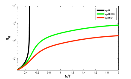
Figure 1: $q_{0}$ as a function of $N/T$ for different values of $\tilde{\eta}$ and $\beta=0.7$.

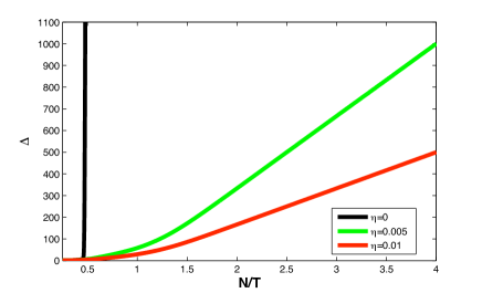
Figure 2: The susceptibility as a function of $N/T$ for different values of $\tilde{\eta}$ and $\beta=0.7$.

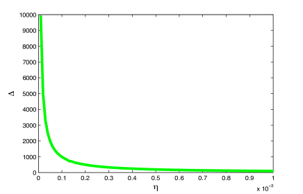
Figure 3: The susceptibility as a function of $\tilde{\eta}$ for the case $t=1.5$ and $\beta=0.7$ .

5 Discussion

Let us now comment on the generality of the result. Concerning the linear assumption in Eq. (6), which is standard in the econometric literature [61], we observe that the estimate of market impact functions is a matter of active current research. Most of the empirical evidence suggests a convex shape [62], with the price impact growing slower than $w$. In double auction markets, if one restricts attention to the instantaneous impact of market orders, the effect on the price depends on the shape of the order book. In order to discuss this case in some more detail, let $\rho_{i}(p,t)$ be the density of limit orders for asset $i$ at time $t$, and consider the situation where a market order for a quantity $w_{i}$ arrives at time $t$. If $p_{i,t-1}$ is the current price and $p_{i,t-1}+x_{i,t}$ is the price (of the transaction which occurred) just before the order arrives, then the price $p_{i,t}$ at which the transaction will take place is given by

$$w_{i}=\int_{p_{i,t-1}+x_{i,t}}^{p_{i,t}}\!dp\rho_{i}(p,t).$$ (23)

A linear impact, as the one assumed in Eq. (6), then corresponds to an order book with a constant density of limit orders. Hence, a measure of $\eta$ is given by the density of the order book close to the best bid/ask. Since the density of the order book fluctuates and liquidity varies across assets, $\eta_{i,t}$ could also be taken as an asset dependent stochastic quantity.

Then the computation of the ES can still be performed in terms of the cost function (9), but now with the $T$ constraints

$$u_{\tau}+v+\sum_{i=1}^{N}w_{i}x_{i,\tau}-\sum_{i}\eta_{i,\tau}w_{i}^{2}\geq 0$$ (24)

in place of Eq. (11). In this case the mapping to a simple $L2$ regularizer that we have laid out in section 3, is then complicated by the fact that the impact term depends on $\tau$ and cannot be absorbed into a $\tau$ independent constant. Nevertheless we do not expect the essential features of the problem to change with respect to the case of a constant $\eta$.

Note furthermore that different assumptions for the market impact function lead to different regularizers. For example, considering the instantaneous impact and Eq. (23), in the presence of a bid-ask spread, we expect the price to bounce from the bid to the ask, depending on the direction of trading (i.e. on the sign of $w_{i}$). This suggests a term proportional to the sign of $w_{i}$ in the equation for the price, which, in turn, would then introduce an $L1$ regularizer. The choice of the regularizer and the behavior of regularized portfolio optimization under the different choices is a rich subject which deserves a separate treatment. However, this choice is related to market impact and liquidity risk considerations.

Notice, finally, that the Maximal Loss limit, $\beta\to 1$, is non-trivial. In this limit, the Expected Shortfall reduces to the Maximal Loss (ML), which reads

$$ML(\mathbf{w})=\max_{t=1,\ldots,T}\left[-\sum_{i}w_{i}x_{i,t}\right].$$ (25)

If we include the market impact term, i.e. if $x_{i,t}\to x_{i,t}-\eta w_{i}$ then

$$ML(\mathbf{w})=\eta\sum_{i}w_{i}^{2}+\max_{t=1,\ldots,T}\left[-\sum_{i}w_{i}x_{i,t}\right],$$

which is clearly finite, for finite $\eta$. However, if the $\beta\to 1$ limit was taken in Eq. (17), one would finds that $C\to\infty$, suggesting that regularization would disappear. The correct limit is recovered (see Appendix) by keeping $T(1-\beta)=1$, i.e. by taking $\beta=1-1/T$, and then eventually letting $T\to\infty$. Therefore, $C=T/2\eta$, which implies that for large $T$ and small $\eta$, liquidity considerations provide only a weak regularizer in the limit of Maximal Loss.

6 Conclusion

We have shown that considering an optimal liquidation policy for a portfolio automatically leads to regularized portfolio optimization. Liquidity considerations provide a way to choose the regularizer. When the market impact is assumed to be linear, we obtain the L2-norm as a regularizer. The typical behavior of large portfolios changes due to the regularization – the otherwise divergent fluctuations in the optimal solution are now tamed. This indicates that regularized portfolio optimization is a better investment strategy for large portfolios than traditional portfolio optimization, which minimizes only the empirical risk.

7 Acknowledgments

I.K. has been supported by the ”Cooperative Center for Communication Networks Data Analysis”, sponsored by the Teller program of the National Office of Research and Technology under grant No. KCKHA005. He is also grateful for the hospitality extended to him at the University of Hawaii at Manoa, Honolulu, during the preparation of this work.

Appendix A The replica calculation

We present here the calculation we use to solve the following optimization problem: find the minimum of the cost function

$$E[\epsilon,\{u_{\tau}\}]=(1-\beta)T\epsilon+\sum_{\tau=1}^{T}u_{\tau}+\tilde{\eta}\|w\|^{2}$$

under the constraints

$$u_{\tau}\geq 0,$$

$$u_{\tau}+\epsilon+\sum_{i=1}^{N}x_{i,\tau}w_{i}\geq 0$$

and

$$\sum_{i}w_{i}=wN.$$

The underlying process governing the returns is assumed to be i.i.d normal. We are using the machinery of statistical physics of random systems, and the terminology will be chosen accordingly. The calculation begins with regarding the cost function as a kind of abstract ”Hamiltonian” or energy functional and introducing a fictitious temperature associated with the system. The reason for this is purely technical, and the original problem will be recovered in the zero temperature limit.

Given a realization for the history of returns $\{x_{i,\tau}\}$, the calculation proceeds by considering the partition function or generating functional

$$Z_{\gamma}(\{x_{i,\tau}\})=\int_{V(\{x_{i,\tau}\})}d\vec{Y}e^{-\gamma E[\vec{Y}]},$$ (26)

where $\gamma$ is the inverse temperature, and we have used the notation $\vec{Y}$ to indicate the set of variables, and $V(\{x_{i,\tau}\})$ represents the portion of phase space where all constraints are satisfied. The minimum cost can then be computed as

$$\lim_{N\to\infty}\lim_{\gamma\to\infty}-\frac{\log Z_{\gamma}(\{x_{i,\tau}\})}{N\gamma}$$ (27)

In order to compute typical properties of the ensemble, we average over the probability distribution of returns, that is we compute the average of $\log Z_{\gamma}(\{x_{i,\tau}\})$. This can be achieved through the replica trick by exploiting the identity

$$\langle\log Z\rangle=\lim_{n\to 0}\frac{\partial Z^{n}}{\partial n}.$$ (28)

The replicated partition function, corresponding to the partition function of $n$ copies of the system can be computed as

$$Z_{\gamma}^{n}[{x_{i,\tau}}] = \int_{-\infty}^{\infty}\prod_{a=1}^{n}d\epsilon^{a}\int_{0}^{\infty}\prod_{\tau=1}^{T}\prod_{a=1}^{n}du_{\tau}^{a}\int_{-\infty}^{\infty}\prod_{i=1}^{N}\prod_{a=1}^{n}dw_{i}^{a}\int_{-\infty}^{\infty}\prod_{a=1}^{n}d\lambda^{a}$$ (29)

$$\times \int_{0}^{\infty}\prod_{\tau=1}^{T}\prod_{a=1}^{n}d\mu_{\tau}^{a}\int_{-\infty}^{\infty}\prod_{\tau=1}^{T}\prod_{a=1}^{n}d\hat{\mu}_{\tau}\exp\left\{\sum_{a}\lambda^{a}(\sum_{i}w_{i}^{a}-wN)\right\}$$ (30)

$$\times \prod_{\tau}\exp\left\{\sum_{a}i\hat{\mu}_{\tau}^{a}\left(u_{\tau}^{a}+\epsilon^{a}+\sum_{i}x_{i,\tau}w_{i}^{a}-\mu_{\tau}^{a}\right)\right\}$$ (31)

$$\times \exp\left\{-\gamma\sum_{a}(1-\beta)T\epsilon^{a}-\gamma\sum_{a,\tau}u_{\tau}^{a}-\gamma\tilde{\eta}\sum_{i}{w_{i}^{a}}^{2}\right\}.$$ (32)

Averaging over the quenched variables $\{x_{i,\tau}\}$ and introducing the overlap matrix $Q_{a,b}=\frac{1}{N}\sum_{i}w_{i}^{a}w_{i}^{b}$ one obtains.

$$Z_{\gamma}^{n}[{x_{i,\tau}}] = \int[D\epsilon][Du][Dw][D\lambda][D\mu][D\hat{\mu}][DQ][D\hat{Q}]\exp\left\{\sum_{a}\lambda^{a}(\sum_{i}w_{i}^{a}-wN)\right\}$$

$$\times \exp\left\{-\gamma\sum_{a}(1-\beta)T\epsilon^{a}-\gamma\sum_{a,\tau}u_{\tau}^{a}-\gamma\tilde{\eta}\sum_{i}{w_{i}^{a}}^{2}\right\}\prod_{\tau}\exp\left\{-\frac{1}{2}\sum_{a,b}\hat{\mu}_{\tau}^{a}Q_{a,b}\hat{\mu}_{\tau}^{b}\right\}$$

$$\times \exp\left\{\sum_{a,b}\hat{Q}_{a,b}\left(NQ_{a,b}-\sum_{i}w_{i}^{a}w_{i}^{b}\right)\right\}$$

$$\times \prod_{\tau}\exp\left\{i\sum_{a}\hat{\mu}_{\tau}^{a}\left(u_{\tau}^{a}+\epsilon^{a}-\mu_{\tau}^{a}\right)\right\}.$$

We can now perform the Gaussian integral over the variables $\{\hat{\mu}_{\tau}^{a}\}$:

$$Z_{\gamma}^{n}[{x_{i,\tau}}] = \int[D\epsilon][Du][Dw][D\lambda][D\mu][DQ][D\hat{Q}]\exp\left\{\sum_{a}\lambda^{a}(\sum_{i}w_{i}^{a}-wN)\right\}$$

$$\times \exp\left\{-\gamma\sum_{a}(1-\beta)T\epsilon^{a}-\gamma\sum_{a,\tau}u_{\tau}^{a}-\gamma\tilde{\eta}\sum_{i}{w_{i}^{a}}^{2}\right\}\exp\left\{\sum_{a,b}\hat{Q}_{a,b}\left(NQ_{a,b}-\sum_{i}w_{i}^{a}w_{i}^{b}\right)\right\}$$

$$\times \prod_{\tau}\exp\left\{-\frac{1}{2}\sum_{a,b}\left(u_{\tau}^{a}+\epsilon^{a}-\mu_{\tau}^{a}\right)Q_{a,b}^{-1}\left(u_{\tau}^{b}+\epsilon^{b}-\mu_{\tau}^{b}\right)\right\}$$

$$\times \exp\left\{-\frac{T}{2}{\rm tr}\log Q\right\}.$$

We are now allowed to perform a Gaussian integration over the variables $\{w_{i}^{a}\}$, which is going to bring the inverse of the operator $\hat{Q}_{a,b}+\gamma\tilde{\eta}\delta_{a,b}$ into the game:

$$Z_{\gamma}^{n}[{x_{i,\tau}}] = \int[D\epsilon][Du][D\lambda][D\mu][DQ][D\hat{Q}]\exp\left\{\sum_{a}-w\lambda^{a}N\right\}$$

$$\times \exp\left\{-\gamma\sum_{a}(1-\beta)T\epsilon^{a}-\gamma\sum_{a,\tau}u_{\tau}^{a}\right\}$$

$$\times \prod_{\tau}\exp\left\{-\frac{1}{2}\sum_{a,b}\left(u_{\tau}^{a}+\epsilon^{a}-\mu_{\tau}^{a}\right)Q_{a,b}^{-1}\left(u_{\tau}^{b}+\epsilon^{b}-\mu_{\tau}^{b}\right)\right\}$$

$$\times \exp\left\{\sum_{a,b}\hat{Q}_{a,b}NQ_{a,b}\right\}\exp\left\{-\frac{T}{2}{\rm tr}\log Q\right\}\exp\left\{-\frac{nN}{2}\log 2\right\}$$

$$\times \exp\left\{-\frac{N}{2}{\rm tr}\log(\hat{Q}+\gamma\tilde{\eta}\delta_{a,b})\right\}\exp\left\{\frac{N}{4}\sum_{a,b}\lambda^{a}\left(\hat{Q}_{a,b}+\gamma\tilde{\eta}\delta_{a,b}\right)^{-1}\lambda^{b}\right\}.$$

Integrating now over the $\{\lambda^{a}\}$ we obtain

$$Z_{\gamma}^{n}[{x_{i,\tau}}] = \int[D\epsilon[Du][D\mu][DQ][D\hat{Q}]\exp\left\{-\gamma\sum_{a}(1-\beta)T\epsilon^{a}-\gamma\sum_{a,\tau}u_{\tau}^{a}\right\}$$

$$\times \prod_{\tau}\exp\left\{-\frac{1}{2}\sum_{a,b}\left(u_{\tau}^{a}+\epsilon^{a}-\mu_{\tau}^{a}\right)Q_{a,b}^{-1}\left(u_{\tau}^{b}+\epsilon^{b}-\mu_{\tau}^{b}\right)\right\}$$

$$\times \exp\left\{N\sum_{a,b}\hat{Q}_{a,b}Q_{a,b}\right\}\exp\left\{-\frac{T}{2}{\rm tr}\log Q\right\}\exp\left\{-\frac{nN}{2}\log 2\right\}$$

$$\times \exp\left\{-\frac{N}{2}{\rm tr}\log(\hat{Q}+\gamma\tilde{\eta}\delta_{a,b})\right\}\exp\left\{-Nw^{2}\sum_{a,b}(\hat{Q}_{a,b}+\gamma\tilde{\eta}\delta_{a,b})\right\}.$$

Introducing the variables $y_{\tau}^{a}=\mu_{\tau}^{a}-u_{\tau}^{b}$ and $z_{\tau}^{a}=\mu_{\tau}^{a}+u_{\tau}^{b}$ and integrating over the $\{z_{\tau}^{a}\}$ one is left with

$$Z_{\gamma}^{n}[{x_{i,\tau}}] = \int[D\epsilon][DQ][D\hat{Q}]$$

$$\times \exp\left\{-Nw^{2}\sum_{a,b}(\hat{Q}_{a,b}+\gamma\tilde{\eta}\delta_{a,b})-\gamma(1-\beta)\sum_{a}T\epsilon^{a}+N\sum_{a,b}\hat{Q}_{a,b}Q_{a,b}\right\}$$

$$\times \exp\left\{-Tn\log\gamma-\frac{T}{2}{\rm tr}\log Q-\frac{N}{2}{\rm tr}\log(\hat{Q}+\gamma\tilde{\eta}\delta_{a,b})-\frac{nN}{2}\log 2\right\}$$

$$\times \exp\left\{T\log Z_{\gamma}(\{\epsilon^{a},Q\})\right\},$$

where we have defined

$$Z_{\gamma}(\{\epsilon^{a},Q\}) = \int\prod_{a}dy^{a}\exp\left\{-\frac{1}{2}\sum_{a,b}(y^{a}-\epsilon^{a})Q_{a,b}^{-1}(y^{b}-\epsilon^{b})\right\}$$

$$\times \exp\left\{\gamma\sum_{a}y^{a}\theta(-y^{a})\right\}.$$

We now take the replica symmetric (RS) ansatz

$$Q_{a,b}=\left\{\begin{array}[]{cc}q_{1},&a=b\\ q_{0},&a\neq b\end{array}\right.$$ (36)

$$\hat{Q}_{a,b}=\left\{\begin{array}[]{cc}\hat{q}_{1},&a=b\\ \hat{q}_{0},&a\neq b.\end{array}\right.$$ (37)

and we define the susceptibility $\Delta q=q_{1}-q_{0}$ as well as $\Delta\hat{q}=\hat{q}_{1}-\hat{q}_{0}$. For $Q^{-1}$ we then have

$$Q_{a,b}^{-1}=\left\{\begin{array}[]{cc}(\Delta q-q_{0})/(\Delta q)^{2}+\mathcal{O}(n),&a=b\\ -q_{0}/(\Delta q)^{2}+\mathcal{O}(n),&a\neq b\end{array}\right.$$ (38)

The effective partition function $Z_{\gamma}(\{\epsilon^{a},Q\})$ reads

$$Z_{\gamma}(\{\epsilon^{a},R^{a},Q\}) = \int\prod_{a}dx^{a}\exp\left\{-\frac{1}{2}\sum_{a,b}x^{a}Q_{a,b}^{-1}x^{b}\right\}$$

$$\times \exp\left\{\gamma\sum_{a}(x^{a}+\epsilon^{a})\theta(-x^{a}-\epsilon^{a})\right\},$$

where we have defined $x^{a}=y^{a}-\epsilon^{a}$. By introducing a Gaussian variable $s$ with measure $dP_{q_{0}}(s)=\frac{ds}{\sqrt{2\pi q_{0}}}e^{-s^{2}/2q_{0}}$ we obtain, in the limit $n\to 0$,

$$\frac{1}{n}\log(Z_{\gamma}(\{\epsilon^{a},Q\})=\frac{q_{0}}{2\Delta q}+\int dP_{q_{0}}(s)\log B_{\gamma}(s,\epsilon,\Delta q),$$

where

$$B_{\gamma}(s,\epsilon,\Delta q)=\int dx\exp\left\{-\frac{(x-s)^{2}}{2\Delta q}+\gamma(x+\epsilon)\theta(-x-\epsilon)\right\}.$$

If we also consider that

$${\rm tr}\log Q=n(\log\Delta q+q0/\Delta q)$$

and

$${\rm tr}\log(\hat{Q}+\gamma\tilde{\eta}\delta_{a,b})=n(\log(\Delta\hat{q}+\gamma\tilde{\eta})+\hat{q_{0}}/(\Delta\hat{q}+\gamma\tilde{\eta})),$$

we finally obtain the free energy

$$-\frac{\gamma F(q_{0},\Delta q,\hat{q_{0}},\Delta\hat{q},\epsilon)}{nN} = q_{0}\Delta\hat{q}+\hat{q}_{0}\Delta q+\Delta q\Delta\hat{q}-w^{2}\left(\Delta\hat{q}+\gamma\tilde{\eta}\right)-\gamma t(1-\beta)\epsilon$$

$$- t\log\gamma+t\int dP_{q_{0}}(s)\log B_{\gamma}(\epsilon,s,R,\Delta q)-\frac{t}{2}\log\Delta q$$

$$- \frac{\log 2}{2}-\frac{1}{2}\left(\log(\Delta\hat{q}+\gamma\tilde{\eta})+\frac{\hat{q}_{0}}{\Delta\hat{q}+\gamma\tilde{\eta}}\right),$$

where we have put $T=tN$. From the saddle point equations for $\hat{q}_{0}$ and $\Delta\hat{q}$ we get

$$\Delta\hat{q}+\gamma\tilde{\eta} = \frac{1}{2\Delta q}$$

$$\hat{q}_{0} = \frac{w^{2}-q_{0}}{2(\Delta q)^{2}}.$$

Exploiting these relations the free energy becomes

$$-\gamma f(\epsilon,q_{0},\Delta q) = -\frac{\gamma F}{nN}=\frac{1}{2}-t\log\gamma-\gamma t(1-\beta)\epsilon$$

$$+ t\int dP_{q_{0}}(s)\log B_{\gamma}(\epsilon,s,R,\Delta q)+\frac{1-t}{2}\log\Delta q+\frac{q_{0}-w^{2}}{2\Delta q}-\gamma\tilde{\eta}q_{0}.$$

Notice that

$$\Delta q=\frac{1}{2N}\sum_{i}(w_{i}^{a}-w_{i}^{b})^{2}$$ (39)

is the squared distance between two approximate solution of the optimization problem, drawn with a Gibbs measure with energy $E$. As $\gamma\to\infty$ the Gibbs measure gets more and more peaked on the optimal solution. If the latter is unique, we expect $\Delta q\to 0$. Indeed, given that the measure is nearly Gaussian, we expect $\Delta q\sim 1/\gamma$. Hence, in the large $\gamma$ limit, it is natural to rescale $\Delta q=\Delta/\gamma$ keeping $\epsilon$ and $q_{0}$ independent of $\gamma$. In this limit we obtain the energy function

$$E = t(1-\beta)\epsilon-\frac{q_{0}-w^{2}}{2\Delta}-\int_{-\infty}^{-\Delta}\frac{dx}{\sqrt{2\pi q_{0}}}e^{-(x-\epsilon)^{2}/(2q_{0})}\left(x+\frac{\Delta}{2}\right)$$

$$+ \frac{t}{2\Delta}\int_{-\Delta}^{0}\frac{dx}{\sqrt{2\pi q_{0}}}e^{-(x-\epsilon)^{2}/(2q_{0})}x^{2}.$$

We now define $\tilde{x}=x/\Delta$, $\tilde{\epsilon}=\epsilon/\Delta$ and $\tilde{q}_{0}=q_{0}/\Delta^{2}$. The reason for this change of variables is that we want to expose the singular behavior at the phase transition in terms of a single divergent quantity $\Delta$. Hence, we anticipate that $\tilde{\epsilon}$ and $\tilde{q}_{0}$ are going to attain finite values at the transition. In terms of the rescaled variables, we have

$$E(\tilde{\epsilon},\tilde{q}_{0},\Delta) = \frac{w^{2}}{2\Delta}+\Delta\left[t(1-\beta)\tilde{\epsilon}-\frac{\tilde{q}_{0}}{2}+\frac{t}{2\sqrt{\pi}}\int_{-\infty}^{\infty}dse^{-s^{2}}g(\tilde{\epsilon}+s\sqrt{2\tilde{q}_{0}})\right]+\tilde{\eta}t\tilde{q_{0}}\Delta^{2}$$

where

$$g(x)=\left\{\begin{array}[]{cc}0,&x\geq 0\\ x^{2},&-1\leq x\leq 0\\ -2x-1,&x<-1\end{array}\right.$$ (40)

and $\tilde{q}_{0}$ and $\tilde{\epsilon}$ are the solutions of the saddle point equations

$$-1+\frac{t}{\sqrt{2\pi\tilde{q}_{0}}}\int dse^{-s^{2}}sg^{\prime}(\tilde{\epsilon}+s\sqrt{2\tilde{q}_{0}})+2\tilde{\eta}\Delta=0,$$ (41)

$$1-\beta+\frac{1}{2\sqrt{\pi}}\int dse^{-s^{2}}g^{\prime}(\tilde{\epsilon}+s\sqrt{2\tilde{q}_{0}})=0,$$ (42)

$$-\frac{w^{2}}{2\Delta^{2}}+t(1-\beta)\tilde{\epsilon}-\frac{\tilde{q}_{0}}{2}+\frac{t}{2\sqrt{\pi}}\int dse^{-s^{2}}g(\tilde{\epsilon}+s\sqrt{2\tilde{q}_{0}})+2\tilde{\eta}\Delta\tilde{q}_{0}=0.$$ (43)

Appendix B The Maximal Loss Problem

We show here how to recover the correct $\beta\to 1$ limit leading to the Maximal Loss problem. The problem of finding the set of weights that minimizes the Maximal Loss (25) can be cast into that of finding the minimum of the cost function

$$E[u]=u$$ (44)

under the constraints

$$u+\sum_{i}w_{i}x_{i,t}\geq 0~{}~{}~{}\forall t$$

and

$$\sum_{i}w_{i}=wN.$$

Let us show how this can be recovered starting from the general problem for the Expected Shortfall

$$E[\epsilon,\{u_{\tau}\}] = (1-\beta)T\epsilon+\sum_{\tau=1}^{T}u_{\tau},$$ (45)

$$u_{\tau} \geq 0~{}~{}\forall\tau,$$ (46)

$$u_{\tau}+\epsilon+\sum_{i=1}^{N}x_{i,\tau}w_{i} \geq 0~{}~{}\forall\tau,$$ (47)

$$\sum_{i}w_{i} = wN.$$ (48)

The first observation is that, for $\epsilon\geq ML$, (47) is satisfied for any set of $\{u_{i,\tau}\}$ satisfying (46). The minimum of the cost function can then be obtained by taking $\epsilon$ equal to the Maximal Loss and $u_{i,\tau}=0~{}\forall i,\tau$. By comparing the resulting expression for (45) with (44), we can see that the two are equivalent if we keep $T(1-\beta)=1$. If we now introduce the regularization, the cost function for the Maximal Loss problem reads

$$E[u,\{w_{i}\}]=u+\frac{T}{2C}\|\vec{w}\|^{2}.$$

As in section 3, an equivalent expression can be obtained by introducing the effect of the price impact. The two approaches are equivalent once we have taken

$$C=\frac{T}{2\eta}.$$ (49)

Notice that one can derive Eq. (49) also by taking $1-\beta=1/T$ in (17), which is indeed the appropriate confidence level for maximal loss, because in a finite time window of $T$ points, the worst possible outcome occurs with probability $1-\beta=1/T$.

References

- [1] E. J. Elton and M. J. Gruber, Modern portfolio theory and investment analysis. Wiley, New York, 1995.
- [2] J. Jobson and B. Korkie, “Improved estimation for Markowitz portfolios using James-Stein type estimators,” Proceedings of the American Statistical Association (Business and Economic Statistics), vol. 1, pp. 279–284, 1979.
- [3] P. Jorion, “Bayes-Stein estimation for portfolio analysis,” Journal of Financial and Quantitative Analysis, vol. 21, pp. 279–292, 1986.
- [4] P. Frost and J. Savarino, “An empirical Bayes approach to efficient portfolio selection,” Journal of Financial and Quantitative Analysis, vol. 21, pp. 293–305, 1986.
- [5] R. Macrae and C. Watkins, “Safe portfolio optimization,” in Proceedings of the IX international symposium of applied stochastic models and data analysis: quantitative methods in business and industry society, ASMDA-99, 14-17 June 1999, Lisbon, Portugal (H. Bacelar-Nicolau, F. C. Nicolau, and J. Janssen, eds.), p. 435, Portugal: INE, Statistics National Institute, 1999.
- [6] R. Jagannathan and T. Ma, “Risk reduction in large portfolios: Why imposing the wrong constraints helps,” Journal of Finance, vol. 58, pp. 1651–1684, 2003.
- [7] O. Ledoit and M. Wolf, “Improved estimation of the covariance matrix of stock returns with an application to portfolio selection.,” Journal of Empirical Finance, vol. 10, no. 5, pp. 603–621, 2003.
- [8] O. Ledoit and M. Wolf, “A well-conditioned estimator for large-dimensional covariance matrices,” J. Multivar. Anal., vol. 88, pp. 365–411, 2004.
- [9] O. Ledoit and M. Wolf, “Honey, i shrunk the sample covariance matrix,” J. Portfolio Management, vol. 31, p. 110, 2004.
- [10] V. DeMiguel, L. Garlappi, and R. Uppal, “Optimal versus naive diversification: How efficient is the 1/n portfolio strategy?,” Review of Financial Studies, 2007.
- [11] L. Garlappi, R. Uppal, and T. Wang, “Portfolio selection with parameter and model uncertainty: a multi-prior approach,” Review of Financial Studies, vol. 20, pp. 41–81, 2007.
- [12] V. Golosnoy and Y. Okhrin, “Multivariate shrinkage for optimal portfolio weights,” The European Journal of Finance, vol. 13, pp. 441–458, 2007.
- [13] R. Kan and G. Zhou, “Optimal portfolio choice with parameter uncertainty,” Journal of Financial and Quantitative Analysis, vol. 42, pp. 621–656, 2007.
- [14] G. Frahm and C. Memmel, “Dominating estimators for the global minimum variance portfolio,” 2009. Deutsche Bundesbank, Discussion Paper, Series 2: Banking and Financial Studies.
- [15] V. DeMiguel, L. Garlappi, F. J. Nogales, and R. Uppal, “A generalized approach to portfolio optimization: Improving performance by constraining portfolio norms.,” Management Science, vol. 55, pp. 798–812, 2009.
- [16] L. Laloux, P. Cizeau, J.-P. Bouchaud, and M. Potters, “Noise dressing of financial correlation matrices,” Phys. Rev. Lett., vol. 83, pp. 1467–1470, 1999.
- [17] V. Plerou, P. Gopikrishnan, B. Rosenow, L. Amaral, and H. Stanley, “Universal and non-universal properties of cross-correlations in financial time series,” Phys. Rev. Lett., vol. 83, p. 1471, 1999.
- [18] L. Laloux, P. Cizeau, J.-P. Bouchaud, and M. Potters, “Random matrix theory and financial correlations.,” International Journal of Theoretical and Applied Finance, vol. 3, p. 391, 2000.
- [19] V. Plerou, P. Gopikrishnan, B. Rosenow, L. A. N. Amaral, T. Guhr, and H. E. Stanley, “A random matrix approach to cross-correlations in financial time-series.,” Phys. Rev. E, vol. 65, p. 066136, 2000.
- [20] Z. Burda, A. Goerlich, and A. Jarosz, “Signal and noise in correlation matrix,” Physica, vol. A343, p. 295, 2004.
- [21] M. Potters and J.-P. Bouchaud, “Financial applications of random matrix theory: Old laces and new pieces,” Acta Phys. Pol., vol. B36, p. 2767, 2005.
- [22] S. Pafka and I. Kondor, “Noisy covariance matrices and portfolio optimization ii,” Physica, vol. A 319, pp. 487–494, 2003.
- [23] I. Kondor, S. Pafka, and G. Nagy, “Noise sensitivity of portfolio selection under various risk measures,” Journal of Banking and Finance, vol. 31, pp. 1545–1573, 2007.
- [24] S.Still and I. Kondor, “Regularizing portfolio optimization,” 2009. To appear on New Journal of Physics. Available on arXiv: 0911.1694.
- [25] C. Cortes and V. Vapnik, “Support vector networks,” Machine Learning, vol. 20, pp. 273–297, 1995.
- [26] B. Schölkopf, A. J. Smola, R. C. Williamson, and P. L. Bartlett, “New support vector algorithms,” Neural Computation, vol. 12, pp. 1207–1245, 05 2000.
- [27] J. Brodie, I. Daubechies, C. D. Mol, D. Giannone, and I. Loris, “Sparse and stable markowitz portfolios,” Proceedings of the National Academy of Science, vol. 106, no. 30, pp. 12267–12272, 2009.
- [28] G. Szegö, ed., Risk measures for the 21st century. J. Wiley and Sons, New York, 2004.
- [29] B. Mandelbrot, “The variation of certain speculative prices,” The Journal of Business of the University of Chicago, vol. 38, pp. 394–419, 1963.
- [30] E. Fama, “The behavior of stock market prices,” Journal of Business, vol. 38, pp. 34–105, 1965.
- [31] U. Muller, M. Dacorogna, R. Olsen, O. Picte, M. Schwartz, and C. Morgenegg, “Statistical study of foreign exchange rates, empirical evidence of a price change scaling law, and intraday analysis,” Journal of Banking and Finance, vol. 14, p. 1189, 1990.
- [32] M. Hols and C. D. Vries, “The limiting distribution of extremal exchange rate returns,” Journal of Applied Econometrics, vol. 6, pp. 287–302, 1991.
- [33] R. Mantegna and E. Stanley, “Scaling behavior in the dynamics of an economic index,” Nature, vol. 376, pp. 46–49, 1995.
- [34] P. Jorion, VaR: the new benchmark for managing financial risk. McGraw-Hill, New York, 2000.
- [35] J. Morgan and Reuters, “Riskmetrics.” Technical Document available at http://www.riskmetrics.com.
- [36] R. T. Rockafellar and S. Uryasev, “Optimization of conditional value-at-risk.,” Journal of Risk, vol. 2, no. 3, pp. 21–41, 2000.
- [37] C. Acerbi, “Spectral measures of risk: a coherent representation of subjective risk aversion.,” Journal of Banking and Finance, vol. 26, no. 7, pp. 1505–1518, 2002.
- [38] C. Acerbi and D. Tasche, “On the coherence of expected shortfall.,” Journal of Banking and Finance, vol. 26, no. 7, pp. 1487–1503, 2002.
- [39] C. Acerbi, “Coherent representations of subjective risk-aversion.,” in Risk Measures for the 21st Century. (G. Szegö, ed.), John Wiley and Sons., 2004.
- [40] P. Artzner, F. Delbaen, J.-M. Eber, and D. Heath, “Coherent measures of risk,” Mathematical Finance, vol. 9, pp. 203–228, 1999.
- [41] P. Embrechts, “Extreme value theory: Potential and limitations as an integrated risk measurement tool.,” Derivatives Use, Trading and Regulation, vol. 6, pp. 449–456, 2000.
- [42] C. Acerbi, C. Nordio, and C. Sirtori, “Expected shortfall as a tool for financial risk management.,” 2001. unpublished.
- [43] J.-P. Bouchaud and M. Potters, Theory of Financial Risk - From Statistical Physics to Risk Management. Cambridge, UK: Cambridge University Press, 2000.
- [44] R. Tibshirani, “Regression shrinkage and selection via the lasso.,” J. Royal. Statist. Soc B., vol. 58, no. 1, pp. 267–288, 1996.
- [45] S. Chen, D. Donoho, and M. Saunders, “Atomic decomposition by basis pursuit,” SIAM Rev., vol. 43, pp. 129–159, 2001.
- [46] N. Gulyas and I. Kondor, “Portfolio instability and linear constraints,” 2007. submitted to Physica A.
- [47] I. Varga-Haszonits and I. Kondor, “The instability of downside risk measures,” J. Stat. Mech., vol. P12007, 2008.
- [48] I. Kondor and I. Varga-Haszonits, “Feasibility of portfolio optimization under coherent risk measures,” 2008. submitted to Quantitative Finance.
- [49] C. Acerbi and G. Scandolo, “Liquidity risk theory and coherent measures of risk,” 2007. Available at SSRN: http://ssrn.com/abstract=1048322.
- [50] S. Ciliberti, I. Kondor, and M. Mezard, “On the feasibility of portfolio optimization under expected shortfall,” Quantitative Finance, vol. 7, pp. 389–396, 2007.
- [51] R. Merton, “On estimating the expected return on the market: An exploratory investigation,” Journal of Financial Economics, vol. 8, pp. 323–361, 1980.
- [52] V. Vapnik and A. Chervonenkis, “On the uniform convergence of relative frequencies of events to their probabilities,” Theory of Probability and its Applications, vol. 16, no. 2, pp. 264–280, 1971.
- [53] V. Vapnik, The Nature of Statistical Learning Theory. Springer Verlag, New York, 1995.
- [54] V. Vapnik, Statistical Learning Theory. John Wiley and Sons, New York, 1998.
- [55] P. J. Huber, Robust Statistics. J. Wiley and Sons, New York, 1981.
- [56] H. Markowitz, “Portfolio selection,” Journal of Finance, vol. 7, pp. 77–91, 1952.
- [57] M. Opper, “Statistical mechanics of learning: Generalization,” in The Handbook of Brain Theory and Neural Networks, (1st edition), pp. 922–925, MIT Press, 1995.
- [58] M. Opper and D. Haussler, “Bounds for predictive errors in the statistical mechanics of supervised learning,” Phys. Rev. Lett., vol. 75, pp. 3772–3775, 1995.
- [59] R. Dietrich, M. Opper, and H. Sompolinsky, “Statistical mechanics of support vector networks,” Phys. Rev. Lett., vol. 82, pp. 2975–2978, 1999.
- [60] D. Malzahn and M. Opper, “A statistical physics approach for the analysis of machine learning algorithms on real data,” Journal of Statistical Mechanics (JSTAT), 2005.
- [61] J. Hasbrouck, “Measuring the information content of stock trades,” Journal of Finance, vol. 46, pp. 179–207, 1991.
- [62] Z. Eisler, J.-P. Bouchaud, and J. Kockelkoren, “The price impact of order book events: market orders, limit orders and cancellations,” 2009. Available on arXiv: 0904.0900.