Diversity, competition, extinction:
the ecophysics of language change

Abstract

As early indicated by Charles Darwin, languages behave and change very much like living species. They display high diversity, differentiate in space and time, emerge and disappear. A large body of literature has explored the role of information exchanges and communicative constraints in groups of agents under selective scenarios. These models have been very helpful in providing a rationale on how complex forms of communication emerge under evolutionary pressures. However, other patterns of large-scale organization can be described using mathematical methods ignoring communicative traits. These approaches consider shorter time scales and have been developed by exploiting both theoretical ecology and statistical physics methods. The models are reviewed here and include extinction, invasion, origination, spatial organization, coexistence and diversity as key concepts and are very simple in their defining rules. Such simplicity is used in order to catch the most fundamental laws of organization and those universal ingredients responsible for qualitative traits. The similarities between observed and predicted patterns indicate that an ecological theory of language is emerging, supporting (on a quantitative basis) its ecological nature, although key differences are also present. Here we critically review some recent advances lying and outline their implications and limitations as well as open problems for future research.

R. V. Solé et al.The ecophysics of language

(ricard.sole@upf.edu)

1 Introduction

Languages and species share some remarkable commonalities. Such similarities did not escape from the attention of Charles Darwin, who mentioned them a number of times in writings and letters (see Whitfield, 2008). In The Descent of Man (Darwin, 1871) he explicitely says:

The formation of different languages and of distinct species, and the proofs that both have been developed through a gradual process, are curiously parallel

Languages indeed behave as some kind of living species (Mufwene 2001; Pagel 2009). They exhibit a large diversity: it is estimated that around $6000$ different languages exist today in our modern world (Krauss, 1992; Nettle and Romaine, 2000; McWorther, 2001). Languages and genes are known to be correlated at both global (Cavalli-Sforza et al. 1988; Cavalli-Sforza, 2000) and local (see Lansing et al., 2007 and references therein) population scales. As it occurs with biodiversity estimates too, the actual language diversity is unknown, and estimates fluctuate up to around $10000$ different spoken languages. Needless to say, another element to consider is the internal diversity displayed by languages themselves, where -like subspecies- dialects abound.

Languages also display geographical variation: as it occurs with species, they become more and more different under the presence of physical barriers. They come to life, as species appear by speciation. They also get extinct, and language extinction has become a major problem to our cultural heritage: as it occurs with endangered species, many languages are also on the verge of disappearance (Crystal, 2000; Sutherland, 2003; Dalby 2003; Mufwene, 2004). Languages die with their last speaker: Crystal mentions the example of Ole Stig Andersen, a researcher looking in 1992 for the last speaker of the West Caucasian language Ubuh. In the words of Andersen:

(The Ubuh) … died at day break, October 8th 1992, when the last speaker, Tevfik Esenç, passed away. I happened to arrive in his village that very same day, without appointment, to interview the Last Speaker, only to learn that he had died just a couple of hours earlier.

This story dramatically illustrates the last breath of any extinct language. It dies as soon as its last speaker dies (or stops using it). It is also interesting to observe that the extinction risk and its correlation with geographical distribution is shared by both species and languages (Sutherland, 2003).

Language change involves both evolutionary and ecological time scales. Most theoretical studies deal with large-scale evolution: how languages emerge and become shaped by natural selection (Hawkins and Gell-Mann 1992; Nowak and Krakauer, 1994; Deacon 1997; Parisi 1997; Cangelosi and Parisi 1998; Pinker 2000; Cangelosi 2001; Kirby 2002; Hauser et al. 2002; Wray 2002; Brighton et al. 2005; Kosmidis et al., 2005, 2006; Baxter et al., 2006; Szamado and Szathmary 2006; Oudeyer and Kaplan 2007; Floreano et al., 2007; Lipson 2007; Christiansen and Chater 2008; Chater et al., 2009; Nolfi and Mirolli 2010). But languages also display changes within the short time scale of one or a few human generations. Actually, a great deal of what will happen to languages in the future is deeply related to their ecological nature. Demographic growth, the dominant role of cities in social and economic organization and globalization dynamics will largely shape world’s languages (Graddol, 2004).

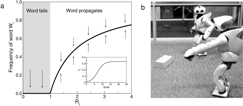
Figure 1: (a) Bifurcations in word learning dynamics: using a simple model of epidemic spreading of words, two different regimes are present. If the rate of word learning exceeds one (i. e. $R_{i}>1$), a stable fraction of the population will use it. If not, then a well-defined threshold is found (a phase transition) leading to word extinction. The inset shows an example of the logistic (S-shaped) growth curve for $R_{i}=1.5$ and $x_{i}(0)=0.01$. Lexical diffusion also occurs in so called naming games among artificial agents (b) where words are generated, communicated and eventually shared by artificial, embodied agents such as robots (picture courtesy of Luc Steels, SONY Labs). As common words get shared, a common vocabulary is generated and eventually stabilized. The dynamics of these exchanges also follows an S-shaped pattern.

Languages evolve under centuries of accumulated modifications (this is well illustrated by written texts, see Howe et al., 2001, Bennett et al, 2003) and undergo evolutionary bursts (Atkinson et al., 2008). On short time scales they can be described in terms of ecological systems. These rapid modifications affect language diversity, their internal differentiation and even their survival. Different studies using the perspective of statistical physics (Nettle 1999a-c; Benedetto et al., 2002; Stauffer and Schulze, 2005; Wang and Minett, 2005; Ke et al., 2002, 2008; Loreto and Steels, 2007; Zanette, 2008; de Oliveira et al., 2008) have been able to cope with these phenomena, showing that the basic trends of language dynamics share remarkable similarities with the spatiotemporal behavior of complex ecosystems.

We will consider different levels of language organization, from words to languages as abstract entities. The models reviewed here explore the conditions under which words or languages can survive or disappear. The time scale is ecological; therefore we assume that in short time scales the dynamics of change does not affect the structure of language itself and thus evolutionary models are not considered. Moreover, we do not intend to quantitatively reproduce observed patterns, although the predictions of the models can be tested in many cases from real data. Instead, the models we revise try to capture the logic of the underlying processes in a qualitative fashion. These models follow the spirit of statistical physics in trying to reduce system’s complexity to its bare bones. They provide a powerful approximation that allow us to see global patterns that might not depend on the intrinsic nature of the components involved. They also help highlighting the differences. As will be discussed below, languages also exhibit marked departures from ecological traits.

This review critically examines a set of models of increasing complexity. Specifically, we review recent advances within the fields of statistical physics and theoretical ecology relative to a better understanding of language dynamics. We begin with a very simple model describing word propagation within a population. Next, the effects and consequences of competition among linguistic variants, with special attention to those scenarios leading to language extinction. This is expanded by considering alternative scenarios allowing language coexistence to occur, either through bilingualism or spatial and social seggregation. Although spatial coexistence under local competition is shared with ecosystems, bilingualism belongs to a different class of phenomenon. All these models involve a small number of interacting languages. The final part of the review deals with language diversity in space and time. Both a simple model of multilingual communities and available data on scaling laws in language diversity are presented. Once again, striking similarities and strong differences are found. A synthesis of these ideas and open problems is presented at the end, together with a table comparing language and ecosystem’s properties.

2 Lexical diffusion

The potential set of words used by a speakers community is listed in dictionaries (Miller, 1991). They capture a given time snapshot of the available vocabulary, but in reality speakers only use part of the possible words: many are technical and thus only used by a given group and many are seldom used. Many words are actually extinct, since no one is using them. On the other hand, it is also true that dictionaries do not include all words used by the community and also that new words are likely to be created constantly within populations and their origins have been sometimes recorded (Chantrell, 2002). Many of them are new uses of previous words or recombinations and sometimes they come from technology. One of the challenges of current theories of language dynamics is understanding how words originate, change and spread within and between populations, eventually being fixed or extinct. In this context, the appearance of a new word has been compared to a mutation (Cavalli-Sforza and Feldman, 1981).

As it occurs with mutational events in standard population genetics, new words or sounds can disappear, randomly fluctuate or get fixed. In this context, the idea that words, grammatical constructions or sounds can spread through a given population was originally formulated by William Wang. It was proposed in order to explain how lexical diffusion (i. e. the spread across the lexicon) occurs (Wang 1969). Such process requires the diffusion of the innovation from speaker to speaker (Wang and Minett 2005).

2.1 Logistic spreading

A very first modeling approximation to lexical diffusion in populations should account for the spread of words as a consequence of learning processes (Shen 1997; Wang et al., 2004; Wang and Minett 2005). Such model should be able to establish the conditions favouring word fixation. As a first approximation, let us assume that each item is incorporated independently (Shen, 1997; Nowak et al., 1999). If $x_{i}$ indicates the fraction of the population knowing the word $W_{i}$, the population dynamics of such word reads:

$${dx_{i}\over dt}=R_{i}x_{i}(1-x_{i})-x_{i},$$ (1)

with $i=1,...,n$. The first term in the right-hand side of the previous equation introduces the way words are learned. The second deals with deaths of individuals at a fixed rate (here normalized to one). The way words are learned involve a nonlinear term where the interactions between those individuals knowing $W_{i}$ (a fraction $x_{i}$) and those ignoring it (a fraction $1-x_{i}$) are present. The parameter $R_{i}$ introduces the rate at which learning takes place.

Two possible equilibrium points are allowed, obtained from $dx_{i}/dt=0$. The first is $x_{i}^{*}=0$ and the second:

$$x_{i}^{*}=1-{1\over R_{i}}.$$ (2)

The first corresponds to the extinction of $W_{i}$ (or its inability to propagate) whereas the second involves a stable population knowing $W_{i}$. The stability of these fixed points is determined by the sign of

$$\lambda(x_{i}^{*})=\left({\partial\dot{x_{i}}\over\partial x_{i}}\right)_{x_{i}^{*}}.$$ (3)

If $\lambda(x^{*})<0$ the point is stable and will be unstable otherwise (Kaplan and Glass, 1995; Strogatz 2001).

The larger the value of $R_{i}$, the higher the number of individuals using the word. We can see that for a word to be maintained in the population lexicon, we require the following inequality to be fulfilled:

$$R_{i}>1.$$ (4)

This means that there is a threshold in the rate of word propagation to sustain a stable population. By displaying the stable population $x^{*}$ against $R_{i}$ (figure 1a) we observe a well-defined phase transition phenomenon: a sharp change occurs at $R_{i}^{c}=1$, the critical point separating the two possible phases. The subcritical phase $R_{i}<1$ will inevitably lead to the loss of the word.

The dynamical pattern displayed by a succesful propagating word follows a so called $S-$shaped curve (see (Niyogi, 2006) and references therein concerning the gradualness and abruptness of linguistic change). This can be easily seen by integrating the previous model. Let us first note that the original equation (1) can be re-writen as a logistic one, namely:

$${dx_{i}\over dt}=(R_{i}-1)x_{i}\left(1-{x_{i}\over x_{i}^{*}}\right),$$ (5)

which, for an initial condition $x_{i}(0)$ at $t=0$, gives a solution

$$x_{i}(t)={x_{i}(0)e^{(R_{i}-1)t}\over 1+x_{i}(0)(e^{(R_{i}-1)t}-1)}.$$ (6)

This curve is known to increase exponentially at low population values, describing a scenario where words rapidly propagate, followed by a slow down as the number of potential learners decays. The accelerated, exponential growth has been dubbed the snowball effect (Wang and Minett, 2005) and such curves have been fitted to available data (Wang 1969). Therefore, a central property of linguistic change, namely its gradualness, can be derived as an epiphenomenon from the dynamical patterns of successful propagation in the case of lexical diffusion. A further issue would to explore whether the gradualness of grammatical (phonological, morphological and syntactical) change can be derived from equations similar to those that model the diffusion of words. It must be noted, from a different perspective, that the logistic trajectory of linguistic change may be favored by “the underlying dynamics of individual learners”, as argued by Niyogi (Niyogi 2006, p. 167).

The previous toy model of word dynamics within populations is an oversimplification, but it illustrates fairly well a key aspect of language dynamics, which is also observed in ecology (Solé and Bascompte, 2006): thresholds exist and play a role (Nowak and Krakauer, 1999). They remind us that, beyond the gradual nature of change that we perceive through our lives (mainly affecting the lexicon) sudden changes are also likely to occur. An important aspect not taken explicitely into account by the previous model is the process of word generation and modification. Words are originated within populations through different types of processes. They become also incorporated by invasion from foreign languages. Once again, the processes of word invasion and origination recapitulate somehow the mechanisms of change in biological populations.

2.2 Multidimensional diffusion

Several modifications and extensions of the previous model have been suggested (Wang et al., 2004). They include considering multiple words involved in the diffusion process. This scenario would take into account the idea that words interact among them in multiple ways, and their diffusion can be constrained or enhanced by these interactions (Wang and Minett 2005). The resulting model describes the dynamics of a given novelty $x_{i}$ and its previous form $y_{i}$ (these can correspond to two word or sounds). Assuming conservation of their relative abundances, i. e. $x_{i}+y_{i}=1$, it is posible to show that a set of equations

$${dx_{i}\over dt}=(1-x_{i})\left[\alpha_{ii}x_{i}+\sum_{j\neq i}^{N}\alpha_{ij}x_{j}\right]$$ (7)

with $i,j=1,...,N$, describes the lexical diffusion process. The matrix elements $\alpha_{ij}$ introduce the coupling rate between a pair $(i,j)$ of words. It is interpreted as the rate at which adoption of the new word $i$ is induced by the frequency of other novel forms of word $j$. As it is formulated, the stable states are all given by $x_{i}^{*}=1$ and thus (not surprisingly) there is no place for extinction, although there exists some evidence for such scenario, where new items spread initially but eventually decay (Ogura, 1993). An interesting extension of this problem could take into account both positive and negative interactions. In this way, not only facilitation (as given by the positive interactions) but also competition would be considered. In other words, it seems reasonable to think that some words should be incompatible with others. This actually matches the problem of species invasion and assembly in multispecies communities (Levins 1968; Case 1990, 1991; Solé et al., 2002). For an exotic species invading a given community to succeed, some community-level constrains need to be satisfied. It would be interesting to see if similar rules apply to the ups and downs of word spreading.

As in the previous subsection, it seems fair to us to pose the question of whether or not grammatical change can be modelled using equations similar to those explored in the study of lexical diffusion. As to multidimensional diffusion, it may be worth considering in future research whether the diffusion of a grammatical object such as a morphological paradigm or a syntactic structure can be described with an equation analogue to eq. (7). It is also worth noting the existence of implicational universals (Greenberg, 1963), which have the shape given a grammatical property x in a language L, we always find a property y in L, as well as the crosslinguistic observation that certain properties tend to entail other properties with overwhelmingly greater than chance frequency, to put it in Greenberg’s famous words. That is, crosslinguistic grammatical change cannot be perfectly mapped into a pure diffusion process: certain properties entail or tend to entail the presence or absence of certain properties, as different words may positively or negatively interact.

2.3 Naming games

A related problem which also involves the generation and spread of words is the so called naming game. The original formulation and implementation of this problem was proposed by Luc Steels as a model for the emergence of a shared vocabulary within a population of agents (Steels, 2001, 2003, 2005; see also Nolfi and Mirolli, 2010). Originally, this approach involved communication between two embodied communicating agents. These agents (figure 1b) are able to visually identify objects from their environment, assign them to randomly generated names which are then sent to the other agent in a speaker-hearer kind of interaction. Exchanges receive a payoff everytime the same word is used by both agents to name a given object. This is done by means of a trial and error process where failures are common at the beginning, as a common emergent lexicon slowly emerges. Specifically, the set of rules are:

1. The speaker selects an object.

2. The speaker chooses a word describing the object from its inventory of word-object pairs. If it doesn’t have a word then it invents one for the object. The speaker transmits the word-object pair to the listener.

3. If the listener has the word-object pair then the transmission is a success. Both agents remove all other words describing the object from their inventory and keep only the single common word.

4. If the listener does not have the word-object pair, then the listener will add this new word to its inventory. And this is recorded as a failure.

Eventually, a shared, stable repertoire gets fixed. The basic rules can be easily mapped into a toy model (the naming game model) involving many agents, by using a statistical physics approach (Baronchelli et al., 2006, 2008). Both hardware and simulated implementations display an S-shaped growth of the vocabulary, although interesting differences arise when we take into account spatial effects and the pattern of relations between agents, describable as a complex network (Steels and McIntyre 2003; Dall’Asta et al., 2006; Lu et al. 2008; Liu et al., 2009).

3 Competition and extinction

Languages are spoken by individuals, and the number of speakers provides a measure of language breadth. Because of both economic and social factors, a given language can become more efficient than others in recruiting new users and as a consequence it can reach a larger fraction or even exclude the second language, which gets extinct. This replacement would be a consequence of competition, one of the most essential components of ecological dynamics, which can be applied to language dynamics too. Early models of two-species competition define the basic formal scenario where species interactions under limited resources occur (Case, 2000). The standard model is provided by the classical Lotka-Volterra equations, namely:

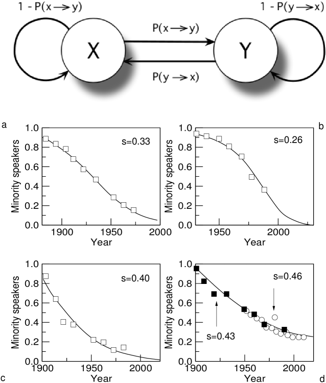
Figure 2: The dynamics of language death. Here four different cases are represented: (a) Scottish Gaelic, (b) Quechua in Huanuco, Peru, (c) Welsh in Monmouthshire, Wales and (d) Welsh in all of Wales, from historical data (filled squares) and a single modern census (open circles). Fitted curves show solutions of the Abrams-Strogatz model (schematically indicated in the upper plot). Redrawn from Abrams and Strogatz, 2003.

$${dx\over dt}=\mu_{1}x(1-x-\beta_{12}y),$$ (8)

$${dy\over dt}=\mu_{2}y(1-y-\beta_{21}x),$$ (9)

where $x$ and $y$ indicate the (normalized) populations of competing species, $\mu_{i}$ indicate their (per capita) growth rates and the coefficients $\beta_{ij}$ are the rates of interspecific competion. We can see that for $\beta_{ij}=0$ two independent logistic equations would be obtained, whereas for non-zero competition two possible scenarios are at work.

Understanding language competition dynamics is clearly important: if the exclusion scenario is also at work, then competition can imply extinction. Moreover, theoretical models can help in defining useful strategies for language preservation and revitalization (Fishman, 1991; 2001). Steady language decline has been observed in some cases, when population records of speakers are available. This is illustrated in figure 2, where the decay over time of four different languages is depicted. All these languages were used by a minority of speakers, competing with a dominant tongue that was gradually adopted by speakers as the less used ones were abandoned. This type of increasing return is common in economics, where positive feedbacks and amplification phenomena are common (Arthur, 1994).

A simple model was proposed by Abrams and Strogatz, which has been shown to provide a rationale for the shape of language decay (Abrams and Strogatz, 2003; Stauffer et al., 2007). The model is based on the assumption that two languages are competing for a given population of potential speakers (the limiting resource) where we will indicate as $x$ and $y$ the relative frequency of each population (assuming that individuals are monolinguals, see below). The dynamics is governed by the following differential equation:

$${dx\over dt}=yP_{\alpha,s}[y\rightarrow x]-xP_{\alpha,s}[x\rightarrow y],$$ (10)

where it is assumed that $P_{\alpha,s}[x\rightarrow y]=0$ if $x=0$ and also constant population ($x+y=1$). The transition probabilities depend on two parameters. The specific model reads:

$${dx\over dt}=s(1-x)x^{\alpha}-(1-s)x(1-x)^{\alpha},$$ (11)

where the $s$ parameter indicates the so called social status of the language. Two extreme equilibrium states are easily found after imposing $dx/dt=0$. These are $x^{*}=0$ (zero population) and $x^{*}=1$ (all speakers use the language). In our case, the stability criterion gives $\lambda(0)=s-1<0$ and $\lambda(1)=-s<0$ and thus both are stable attractors.

Together with the exclusion points $x=0$ and $x=1$, there is a third equilibrium point, which can be obtained from:

$$s{x^{*}}^{\alpha-1}=(1-x^{*})^{\alpha-1}(1-s),$$ (12)

and, after some algebra one finds that:

$$x^{*}=\left[1+\left({s\over 1-s}\right)^{1\over\alpha-1}\right]^{-1}.$$ (13)

Given the stable character of the other two fixed points, $x^{*}$ can only be unstable and thus no coexistence is allowed.

The model has been used to fit available data on language decay (figure 2) and assumes a scenario of minority languages competing with widely used, majority tongues. One clear implication of the stability analysis is that the extinction of one of the competing solutions is inevitable. The social parameter will influence which language will get extinct. Nonetheless, linguistic diversification seems unavoidable: the language that succeeds in the competition situation will become more and more diverse as it extends through time and space, and it may end up yielding mutually unintelligible linguistic variants.

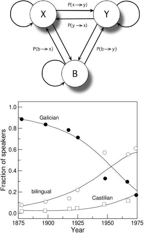
Figure 3: Dynamics of language use under the presence of bilingual speakers. Here three types of speakers are considered (a). In (b) we show the fraction of speakers vs. time in Galicia (North Western Spain). The smooth curves (modified after Mira and Paredes, 2005) are the result of fitting a modified Abrams-Strogatz model (see text).

The AS model does not take into account that a fraction of individuals is likely (under some circumstances) to become bilingual. It might seem a not so relevant item, but bilingualism actually introduces a very interesting ingredient to our view of language change, to be outlined in the next section.

4 Coexistence and bilingualism

The previous model is simplified in many respects. By considering human populations as homogeneous systems, geographical effects and some idiosyncracies of human language (not shared with ecosystems) are ignored. Spatial effects will be explored in the next section. Here we concentrate on a special property of human communities, namely the presence of individuals who are grammatically and communicatively competent on more than one language. Actually, a large fraction of humankind uses more than one tongue for communication. Historical reasons and the influence of modern invasions by languages like English makes multilingualism an important ingredient to take into account.

The Abrams-Strogatz model can be easily expanded (figure 3a) by assuming that two languages are present but bilingual speakers are also allowed (Mira and Paredes, 2005; Castelló et al., 2006; see also Minett and Wang 2008). The basic idea behind this approach is that the presence of bilingual speakers makes language coexistence likely to occur, provided that the two languages are close enough to each other. In this picture, three variables are used: as in the AS model, $x$ and $y$ will be the fraction of speakers using languages $X$ and $Y$. Moreover, a third group $B$ using both languages has a size $b$ in such a way that $x+y+b=1$. Transitions are defined in similar ways (figure 3a). For example, changes in $x$ would result from a kinetic equation:

$${dx\over dt}=yP[y\rightarrow x]+bP[b\rightarrow x]-x\left(P[x\rightarrow y]+P[x\rightarrow b]\right),$$ (14)

and the constant population constraint allows defining the model in terms of just two coupled equations, namely:

$${dx\over dt}=c\left((1-x)(1-\kappa)s_{x}(1-y)^{\alpha}-x(1-s_{x})(1-x)^{\alpha}\right);$$ (15)

$${dy\over dt}=c\left((1-y)(1-\kappa)(1-s_{x})(1-x)^{\alpha}-ys_{x}(1-y)^{\alpha}\right),$$ (16)

where $\kappa\in[0,1]$ is a new parameter measuring the degree of similarity among languages and the language status are now indicated as $s_{x}$ and $s_{y}=1-s_{x}$, respectively. The $\kappa$ parameter provides a measure of the likelihood that two single-language speakers can communicate with each other. It also affects the probability that a monolingual speakers becomes bilingual. We can easily check that the model reduces to the AS scenario for $\kappa=b=0$.

Available data from language change in Northern Spain (Mira and Paredes, 2005) provide a test of this model. Here the two languages are Castilian and Galician, both derived from Latin. These languages allow a relatively good mutual understanding and parameters are easily estimated. For this data set, a best fit was obtained using $a=1.5,s(Galician)=0.26,c=0.1$ and $\kappa=0.8$. As we can see, the apparent decline of Galician is actually a consequence of a simultaneous increase of Castilian monolinguals and bilinguals.

We should be aware of the overestimation of the role of the $\kappa$ parameter as a measure of the probability that a monolingual speaker becomes bilingual, since $\kappa$ is only an indicator of the degree of similarity among languages, and neglects the role of their social status. It is worth noting that many bilingual scenarios involve two highly differentiated languages, such as Basque and Castilian in northern Spain or Amazigh and Arabic in northern Africa.

How likely is the bilingual scenario to be relevant in the future? Recent model approaches suggest that maintaining a bilingual society necessarily requires the maintenance of status as a control parameter (Chapel et al. 2010). On the one hand, preserving language diversity in a globalized world will need active efforts when small populations of speakers are involved. But on the other hand, we must also take into account current demographic trends (Graddol, 2004) which will need to be incorporated into future models of language change. Against early predictions suggesting the dominant role of English as an exclusive language, the future looks multilingual. Different languages are gaining relevance as their social and economic status improves. Moreover, other interesting tendencies start to develop as some languages (such as English, Portuguese or Dutch) spread beyond their original geographic domains. They not only become mutualistic (as a bilingual speaker acquires a higher social status) but can also develop internal differentiation. We should expect in the future to see the emergence of (perhaps uintelligible) dialects of English, as it happened with Latin.

5 Spatial dynamics

The exclusion point resulting from the Lotka-Volterra equation and related models (such as Abrams-Strogatz’s model) implies that strong competition leads to diversity reduction. Within the context of population dynamics, such result was challenged under the introduction of spatial degrees of freedom (Solé et al., 1993; see also Solé and Bascompte, 2007 for a review of results). Spatial dynamics involves two basic components. One is the reaction term, describing how populations interact (for example the previous equations described above). The second describes how populations move through space. It is well known that space is responsible for the emergence of qualitative changes in dynamical patterns (Turing, 1952; Bascompte and Solé, 2000; Dieckmann et al., 2000). Competition under spatial structure generates a completely novel result: since exclusion depends on initial conditions, the two potential attractors can be (locally) possible. Starting from random initial conditions, different species or languages can exclude each other at different locations.

The extension of the Abrams-Strogatz model to space was performed by Patriarca and Leppänen (2004) who used a reaction-diffusion framework. The model considers the local dynamics of the normalized densities of speakers using a given language at each point ${\bf r}$ in space. If $\phi_{x}({\bf r},t)$ and $\phi_{y}({\bf r},t)$ indicate the local densities of $x$ and $y$ at a given point and time, they read:

$${\partial\phi_{x}({\bf r},t)\over\partial t}=F(\phi_{x},\phi_{y})+D_{x}\nabla^{2}\phi_{x}({\bf r},t)$$ (17)

$${\partial\phi_{y}({\bf r},t)\over\partial t}=-F(\phi_{x},\phi_{y})+D_{y}\nabla^{2}\phi_{y}({\bf r},t),$$ (18)

where $F(\phi_{x},\phi_{y})$ is just the AS equation for the local densities:

$$F(\phi_{x},\phi_{y})=s_{x}\phi_{y}\phi_{x}^{\alpha}-s_{y}\phi_{x}\phi_{y}^{\alpha},$$ (19)

and $s_{x},s_{y}$ indicate the status of each language. The $D_{i}$’s on the right side of the equation are the so called diffusion coefficients associated to the spreading process.

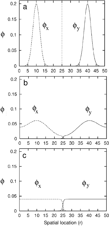
Figure 4: Spatial segregation of languages over time. Here we use the discretized equations of two competing languages in order to calculate their population of speakers (relative frequency) over time. We start in (a) from two segregated populations of speakers, each in a different domain and having a Gaussian shape, with $N_{x}(0)=N_{y}(0)=1/2$, $\alpha=1.3$ and status parameters fixed to $s_{x}=1-s_{y}=0.55$. As we can see (see text) although locally there is exclusion of one language, globally both languages coexist. As time proceeds (b-c) the spatial distribution converges to a homogeneous state where each language survives in each domain. Here $t(b)=10^{3}$ and $t_{c}=10^{4}$.

The previous equations can be numerically integrated (Dieckmann et al., 2000). We will illustrate this by using a one-dimensional spatial system (the generalization to two dimensions is straightforward). First, we discretize $\partial\phi/\partial t$ as follows:

$${\partial\phi_{x}(r,t)\over\partial t}\approx{\phi(r,t+\Delta t)-\phi(r,t)\over\Delta t},$$ (20)

where $r$ is the local position in the one-dimensional domain $Z=[0,L]$ and $\Delta t$ some characteristic time scale. Similarly, the discretization of the diffusion term is made as follows:

$${\partial^{2}\phi_{x}(r,t)\over\partial r^{2}}\approx{\phi(r+\Delta r,t)+\phi(r-\Delta r,t)-2\phi(r,t)\over\Delta r^{2}},$$ (21)

being $\Delta r$ the corresponding characteristic spatial scale. Using these definitions, we obtain an equation for the time evolution of $\phi_{x}(r,t)$:

$$\phi_{x}(r,t+\Delta t) = \phi_{x}(r,t)+$$

$$\left[F(\phi_{x},\phi_{y})+{D\over\Delta r^{2}}(\phi(r+\Delta r,t)+\right.$$

$$\left.+\phi(r-\Delta r,t)-2\phi(r,t))\right]\Delta t.$$

Additionally, boundary conditions need to be included. These allow defining the impact of finite size effects and geography on the dynamics and equilibrium states. The reasonable assumption is to use zero-flux (von Neumann) boundary conditions, namely

$$\left({\partial\phi_{x}(r,t)\over\partial r}\right)_{r=0}=\left({\partial\phi_{x}(r,t)\over\partial r}\right)_{r=L}=0.$$ (22)

In terms of our discretization, we would have $\phi_{x}(0,t)-\phi_{x}(\Delta r,t)=0$ and $\phi_{x}(L,t)-\phi_{x}(L-\Delta r,t)=0$.

The dynamics starts with two populations of speakers located in two different domains $Z_{x}$ and $Z_{y}$ (so that $Z=Z_{y}\cup Z_{y}$). This is shown in figure 4a, where we display the initial condition. If we label as $N_{x}^{\mu}$ and $N_{y}^{\mu}$ the total populations of speakers in each domain $\mu=1,2$, at a given domain $Z_{\mu}$ we would have:

$$N_{i}^{\mu}(t)=\int_{Z_{\mu}}\phi_{i}(r,t)dr,$$ (23)

starting from $N_{i}=1/2$ following a Gaussian shape (see Patriarca and Leppänen, 2004). As the dynamics proceeds, we can observe a tendency towards maintaining the spatial seggregation. Each language “wins” in its initial domain, and eventually both reach a homogeneous steady state within such domain. Generalizations to heterogeneous domains reveal that the previous patterns can be affected by both historical events and spatial inhomogeneities (Patriarca and Heinsalu, 2008). However, the main message from this approach is robust and completely related to models of competing populations in ecology (Solé et al., 1993; Solé and Bascompte 2006). In summary, this tells us that the effects of spatial degrees of freedom on language dynamics have a great impact on the coexistence versus extinction scenarios.

Space slows down the effects of competitive interactions, effectively reducing competition at the local scale. Moreover, the role of diffusion (dispersal) on competition dynamics allows to create well-defined domains where given languages or species have replaced others. In this context, it is clear that the increasing connectivity of our world due to globalization has made easier to reduce the potential impact of geography in the propagation of languages or epidemics (Buchanan, 2003). Although we do live in a two-dimensional surface, the world has certainly changed and spatial constraints have been strongly reduced.

6 String models of language change

As already mentioned in section 2, a collection of words provides a first definition of a language in terms of its lexicon. This of course ignores a crucial component of language: words interact in non-random ways and higher-order levels of organization should be taken into account. However, as it occurs with some theoretical models of diverse ecosystems (Solé and Bascompte, 2006) some relevant problems such as diversity and its maintenance can be properly addressed by ignoring interactions. Following this picture, we consider in this section the lexical component of language viewed as a bag of words and how a set of languages competing for a given population of speakers can evolve towards a single, dominant tongue or instead a diverse set of coexisting languages.

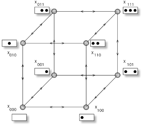
Figure 5: String language model. Here a given set of elements defines a language. Each (possible) language is defined by a string of $\nu$ bits (here $L=3$) and thus $2^{L}$ possible languages are present in the hypercube. The two types of elements are indicated as filled ($1$) and empty ($0$) circles, respectively.

A fruitful toy model of language change is provided by the string approximation (Stauffer et al., 2006; Zanette, 2008). In this approach, each language ${\cal L}_{i}$ is treated as a binary string, i. e. ${\cal L}_{i}=(S^{i}_{1},S^{i}_{2},...,S^{i}_{L})$ of length $L$. Here $S^{i}_{j}\in\{0,1\}$ and, as defined, a finite but very large set of potential languages exists. Specifically, a set of languages ${\bf\cal L}$ is defined, namely

$${\bf\cal L}=\{{\cal L}_{1},{\cal L}_{2},...,{\cal L}_{M}\},$$ (24)

with $M=2^{L}$. These languages can be located as the vertices of a hypercube, as shown in figure 5 for $L=3$. Nodes (languages) are linked through arrows (in both directions) indicating that two connected languages differ in a single bit. This is a very small sized system. As $L$ increases, a combinatorial explosion of potential strings takes place.

6.1 Mean field model

A given language ${\cal L}_{i}$ is shared by a population of speakers, to be indicated as $x_{i}$, and such that the total population of speakers using any language is normalized (i. e. $\sum_{i}x_{i}=1$). A mean field model for this class of description has been presented by Damian Zanette, using a number of simplifications that allow understanding the qualitative behavior of competing and mutating languages (Zanette, 2008). A few basic assumptions are made in order to construct the model. First, a simple fitness function $\phi(x)$ is defined. This function measures the likelihood of abandoning a language. This is a decreasing function of $x$, and such that $\phi(0)=1$ and $\phi(1)=0$. Different choices are possible, including for example $1-x,1-x^{2}$ or $(1-x)^{2}$. On the other hand, mutations are also included: a given language can change if individuals modify some of their bits.

The mean field model considers the time evolution of populations assuming no spatial interactions. If we indicate ${\bf x}=(x_{1},...,x_{M})$, the basic equations will be described in terms of two components:

$${dx_{i}\over dt}=A_{i}({\bf x})-M_{i}({\bf x}),$$ (25)

where both language abandonment $A_{i}({\bf x})$ and mutation $M_{i}({\bf x})$ are introduced. Specifically, the following choices are made:

$$A_{i}({\bf x})=\rho x_{i}\left(\langle\phi\rangle-\phi(x_{i})\right),$$ (26)

for the population dynamics of change due to abandonment. This is a replicator equation, where the speed of growth is defined by the difference between average fitness $\langle\phi\rangle$, namely

$$\langle\phi\rangle=\sum_{j=1}^{N}\phi(x_{j})x_{j},$$ (27)

and the actual fitness $\phi(x_{i})$ of the $i$-language. Here $\rho$ is the recruitment rate (assumed to be equal in all languages). What this fitness function introduces is a multiplicative effect: the more speakers that use a given language, the more likely that they keep using it and others join the same group. Conversely, if a given language is rare, its speakers might easily shift to some other, more common language.

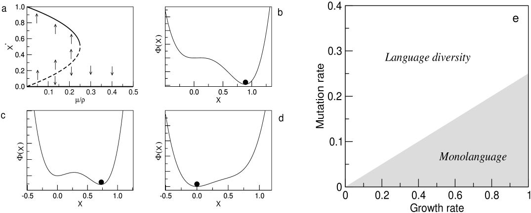
Figure 6: Phase transitions as bifurcations in Zanette’s mean field model of supersymmetric language competition. In (a) we show the bifurcation diagram using $\mu/\rho$ as control parameter. Once we cross the critical point, a sharp transition occurs from monolanguage to language diversity. This transition can be visualized using the potential function $\Phi(x)$ whose minima correspond to possible equilibrium points. Here we use $\rho=1$ with (b) $\mu=0.1$, (c) $\mu=0.2$ and (d) $\mu=0.3$. In (e) we also plot the phase diagram using the $(\rho,\mu)$ parameter space.

The second term includes all possible flows between “neighboring” languages. It is defined as:

$$M_{i}({\bf x})={\mu\over L}\left(\sum_{j=1}^{N}W_{ij}x_{j}-x_{i}\sum_{j=1}^{N}W_{ji}\right).$$ (28)

In this sum, we introduce the transition rates $W_{ij}$ of mutating from language ${\cal L}_{i}$ to language ${\cal L}_{j}$ and vice versa. Only single mutations are allowed, and thus $W_{ij}=1$ if the Hamming distance $D({\cal L}_{i},{\cal L}_{j})$ is exactly $1$. More precisely, if

$$D({\cal L}_{i},{\cal L}_{j})=\sum_{k=1}^{L}|S^{i}_{k}-S^{j}_{k}|=1.$$ (29)

In other words, only nearest-neighbor movements through the hypercube are allowed. In summary, $A({\bf x})$ provides a description of competitive interactions whereas $M({\bf x})$ gives the contribution of small changes in the string composition. The background “mutation” rate $\mu$ is weighted by the matrix coefficients $W_{ij}$ associated with the likelihood of each specific change to occur.

This model is a general description of the bit string approximation to language dynamics. However, the general solution cannot be found and we need to analyse simpler cases. An example is provided in the next section. Although the assumptions are rather strong, numerical models with more relaxed assumptions seem to confirm the basic results reported below.

6.2 Supersymmetric scenario

A solvable limit case with obvious interest to our discussion considers a population where a single language has a population $x$ whereas all others have a small, identical size, i. e. $x_{i}=(1-x)/(N-1)$. The main objective of defining such supersymmetric model is making the previous system of equations collapse into a single differential equation, which we can then analyze. In particular, we want to determine when the $x=0$ state will be observed, meaning that no single dominant language is stable.

Since we have the normalization condition, now defined by:

$$\sum_{j=1}^{N}x_{j}=x+\sum_{j=1}^{M-1}\left({1-x\over N-1}\right)=1$$ (30)

(where we choose $x$ to be the $M$-th population, without loss of generality). In this case the average fitness reads:

$$\langle\phi\rangle=\phi(x)x+\sum_{j=1}^{M-1}\phi\left({1-x\over N-1}\right)\left({1-x\over N-1}\right).$$ (31)

Using the special linear case $\phi(x)=1-x$, we obtain:

$$A(x)=\rho x(1-x)\left(x-{1-x\over N-1}\right).$$ (32)

The second term is easy to obtain: since $x$ has (as any other language) exactly $L$ nearest neighbors, and given the symmetry of our system, we have:

$$B(x)={\mu\over L}\left(L{1-x\over N-1}-xL\right)=-\mu\left({Nx-1\over N-1}\right).$$ (33)

And the final equation for $x$ is thus, for the large-$N$ limit (i. e. when $N\gg 1$):

$${dx\over dt}=\rho x^{2}(1-x)-\mu x.$$ (34)

This equation describes an interesting scenario where growth is not logistic, as it happened with our previous model of word propagation. As we can see, the first term in the right-hand side involves a quadratic component, indicating a self-reinforcing phenomenon. This type of model is typical of systems exhibiting cooperative interactions and an important characteristic is its hyperbolic dynamics: instead of an exponential-like approximation to the equilibrium state, a very fast approach takes place.

The model has three equilibrium points: (a) the extinction state, $x^{*}=0$ where the large language disappears; (b) two fixed points $x_{\pm}^{*}$ defined as:

$$x_{\pm}^{*}={1\over 2}\left(1\pm\sqrt{1-{4\mu\over\rho}}\right).$$ (35)

As we can see, these two fixed points exist provided that $\mu<\mu_{c}=\rho/4$. Since three fixed points coexist in this domain of parameter space, and the trivial one ($x^{*}=0$) is stable, the other two points, namely $x_{-}^{*}$ and $x_{+}^{*}$, must be unstable and stable, respectively. If $\mu<\mu_{c}$, the upper branch $x_{+}^{*}$ corresponding to a monolingual solution, is stable.

In figure 3a we illustrate these results by means of the bifurcation diagram using $\rho=1$ and different values of $\mu$. In terms of the potential function we have:

$${dx\over dt}=-{\partial\Phi_{\mu}(x)\over\partial x},$$ (36)

where $\Phi_{\mu}(x)=-\int(A(x)-B(x))dx$, which for our system reads:

$$\Phi_{\mu}(x)=-\rho\left({x^{3}\over 3}+{x^{4}\over 4}\right)+\mu{x^{2}\over 2}.$$ (37)

In fig 5a-d three examples of this potential are shown, where we can see that the location of the equilibrium point is shifted from the monolanguage state to the diverse state as $\mu$ is tuned. The corresponding phases in the $(\rho,\mu)$ parameter space are shown in figure 5.

It is interesting to see that this model and its phase transition is somewhat connected to the error threshold problem associated to the dynamics of RNA viruses (Domingo et al. 1995; Eigen et al., 1987). For a single language to maintain its dominant position, it must be efficient in recruiting and keeping speakers. But it also needs to keep heterogeneity (resulting from “mutations”) at a reasonable low level. If changes go beyond a given threshold, there is a runaway effect that eventually pushes the system into a variety of coexisting sub-languages. An error threshold is thus at work, but in this case the transition is of first order. This result would indicate that, provided that a source of change is active and beyond threshold, the emergence of multiple uninteligible tongues should be expected.

String models of this type only capture one layer of word complexity. Perhaps future models will consider ways of introducing further internal layers of organization described in terms of superstrings. Such superstring models should be able to introduce semantics, phonology and other key features that are known to be relevant. An example in this direction is provided by models of the emergence of linguistic categories (Puglisi et al., 2008).

7 Global patterns and scaling laws

Tracking the relative importance of languages and in particular their likelihood of getting extinct requires having the appropriate censuses of number of speakers using each language. The statistical patterns displayed by languages in their spatial and demographic dimensions provide further clues for the presence of non-trivial links between language and ecology (Nettle 1998; Pagel and Mace, 2004; Pagel 2009). These patterns also provide a large-scale picture of languages, not restricted to small geographical domains or countries. In this section we consider two of such statistical patterns. It is important to notice that, strictly speaking, this problem involves both ecological and evolutionary time scales. In a given ecosystem, the succession process leading to a mature, diverse community can be described in terms of ecological dynamics. At this level, invasion and network species interactions are both relevant. However, the composition of the local pool of species is the outcome of evolutionary dynamics.

Some spatial models of language change have been presented in order to explain the results shown below (see de Oliveira et al. 2005; de Oliveira et al, 2008). The close correlation between species diversity and language richness, as reported by different studies (Mace and Pagel, 1995; Moore at al., 2002; Gaston 2005) suggests that some rules of organization might be common. As an example, a large scale study of correlations among biological species and cultural and linguistic diversity in Africa (Moore et al., 2002) revealed that one third of language richness can be explained on the basis of environmental factors. These included rainfall and productivity, which were shown to affect the distributions of both species and languages. However, there are also important differences that need an explanation.

7.1 Species-area relations

One of the universal laws of ecological organization is the so called species-area relation (Rosenzweig, 1995). It establishes that the diversity $D$ (measured as the number of different species) in a given area $A$ follows a power law

$$D\sim A^{z},$$ (38)

where the exponent $z$ tipically varies from $z=0.1$ to $z=0.45$. Interestingly, languages seem to follow similar trends. They exhibit an enormous diversity, strongly tied to geographical constraints. As it occurs with species distributions, languages and their evolution are shaped by the presence of physical barriers, population sizes and contingencies of many kinds. In this context, differences are also clear: speciation in ecosystems can take place without the presence of physical barriers, whereas some type of population isolation seems necessary for one language to yield two diferent languages, i.e., two linguistic variants that are not fully interintelligible. On the other hand, there is a continuous drift in both species and languages that makes them change. A second difference involves the way extinction occurs. Species get extinct once the last of its members is gone. Languages get extinct too once they are not used anymore, even if its native speakers are still alive (Dalby, 2005).

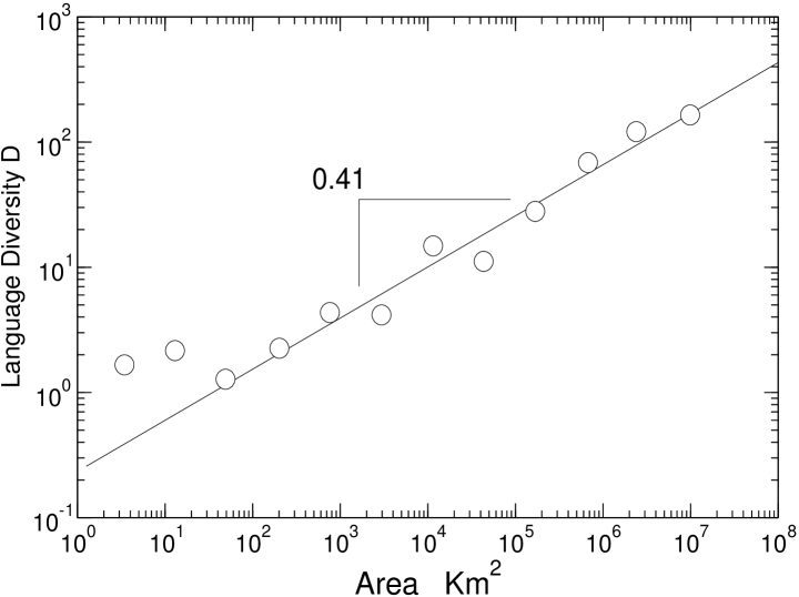
Figure 7: Scaling law in the distribution of language diversity $D$ as a function of area. The best fit to the power law $D\sim A^{z}$ is shown. Redrawn from Gomes et al., 1999.

Studies of geographical patterns of language distribution reveal complex phenomena at multiple scales. As an example, it was shown that they also display a diversity-area scaling law, with $z=0.41\pm 0.03$ (Gomes et al., 1999). In figure 7 we show the results of this analysis for a compilation listing more than 6700 languages spoken in 228 countries. The power law fit is very good and spans over almost six decades (with a deviation for areas smaller than $30Km^{2}$) (Gomes et al., 1999). Similar results are obtained by using population size $N$ instead of areas. In this case, it was shown that the new power law reads:

$$D\sim N^{\nu}$$ (39)

with $\nu=0.50\pm 0.04$. However, a close inspection of data reveals the impact of other forces acting on language diversity. An example is the contrast between Europe and New Guinea (see Diamond, 1997 and references therein). The former has $10^{7}Km^{2}$ and includes 63 languages, whereas the later, with only less than one tenth of Europe’s surface, contains around $10^{3}$ different languages. The singularity of New Guinea has been carefully analysed by many authors. Take for example Papua New Guinea, which contains just $0.1$ percent of the world’s population but more than $13$ percent of world’s languages. It is geographically an extremely irregular landscape, which creates multiple opportunities for isolation. Moreover, $80$ percent of its land is covered by rainforests. Additionally, food production is continuous, with no food shortages and a good yield. Bilingualism is widespread, with most speakers of the dominant Tok Pisin also speaking some local language too (being exposed to several). Given the high yields of food harvest together with biogeographical constraints, there has been little incentive to create large-scale trade. A consequence of such scenario is a dynamic equilibrium far from language homogeneization (see Nettle and Romaine, 2000 for a review).

The species-area relation has been explained in a number of ways through models of population dynamics on two-dimensional domains. Beyond their differences, these models share the presence of stochastic dynamics involving multiplicative processes. In ecology, such type of processes are characterized by positive and negative demographical responses proportional to the current populations involved: a larger population will be more likely to increase, but also more likely to suffer the attack of a given parasite (and thus experience a rapid decline). Within language, the rich-gets-richer effect is obvious, whereas there is no equivalent for the negative effects of “parasitic” languages.

7.2 Language richness laws

A different measure of language diversity involves the language richness among different countries. If ${\cal N}(D)$ is the frequency of countries with $D$ diferent languages each, we can plot the cumulative distribution ${\cal N}_{>}(D)$ defined as:

$${\cal N}_{>}(D)=\int_{D}^{\infty}{\cal N}(D)dD.$$ (40)

The resulting plot is rather interesting (fig 8a): the distribution follows a two-regime scaling behavior, i. e.

$${\cal N}_{>}(D)\sim D^{-\beta},$$ (41)

with $\beta=0.6$ for $6<D<60$ and $\beta=1.1$ for $60<D<700$. What is revealed from this plot? The first domain has an associated power law with a small exponent (here ${\cal N}(D)\sim D^{-1.6}$): many countries have a small language diversity. But once we cross a given threshold $D\approx 60$ the decay becomes faster. One possible interpretation is that countries having a very large diversity will have harder times to preserve their unity under the social differentiation associated to ethnic diversity (Gomes et al., 1999).

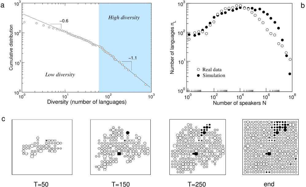
Figure 8: Scaling laws in language diversity. (a) Here we plot the cumulative distribution of languages using the number of countries with a language diversity greater than $D$. Redrawn from Gomes et al., 1999. The marked area indicates the domain of language-rich countries, whose distribution is steeper than the low-diversity domain. (b) Distribution of languages having $N$ speakers. Here the data set for languages is compared with a simulation using a specific set of parameters (see de Oliveira et al, 2008). Although different parameter sets give different curves, the qualitative behavior is allways the same. In (c) we show four snapshots of a model of language diversity dynamics on a two-dimensional lattice (adapted from de Oliveira et al., 2008). Here each symbol type indicates one given language, whereas its size indicates the local population allowed. As time proceeds, mutations arise and new languages emerge and spread (see text).

A related distribution is given by the number of languages $n_{L}(N)$ with a population size of $N$ speakers. In figure 8b we display a log-log plot of the data set (after binning) which shows a log-normal behavior, with an enhanced number of small-sized languages. This pattern (as well as the scaling with area) is reproduced by a simple model presented below.

7.3 Language diversity model

A simple spatial model has been proposed in (de Oliveira et al., 2008) as an extension of previous work (de Oliveira et al., 2006; see also Silva and Oliveira, 2008). The model combines a stochastic cellular automaton approach with non-local rules and a bit-string implementation. Starting from an empty lattice $\Omega$ of $L\times L$ sites. Each site $(i,j)\in\Omega$ is characterized by a random number $1\leq K_{ij}\leq M$ (with uniform distribution) representing the maximum population of speakers achievable by the language occupying it (the carrying capacity). Only one language ${\cal L}_{i}$ can be present at a given site and (as in section 6) is represented by a string ${\cal L}_{i}=(S^{i}_{1},S^{i}_{2},...,S^{i}_{L})$ of length $L$. A seed ${\cal L}_{1}$ is located at $t=0$ at a given site $(a,b)$, thus having a population $K_{ab}$. Now dispersal to nearest neighbors in the lattice occurs, favouring the spread towards sites having higher $K_{ij}$. Moreover, at a given site the given language ${\cal L}_{k}$ can change (mutate) to a new one with a probability $\mu_{k}=\alpha/f({\cal L}_{k})$. Here $f({\cal L}_{k})$ is the fitness associated to ${\cal L}_{k}$, here chosen as:

$$f({\cal L}_{k})=\sum_{i,j}K_{ij}\theta({\cal L}(i,j),{\cal L}_{k})$$ (42)

with $\theta(m,n)=1$ if $m=n$ and zero otherwise. In words, the fitness considers the total occupation of the lattice (in terms of speakers), and the likelihood of a language to mutate is thus size-dependent following an inverse law. In this way we incorporate the well known fact that the impact of mutations favour genetic drift. The previous rules allow a diverse set of languages to expand and eventually occupy the whole lattice. An example is shown in figure 8b for a small ($L=50$) lattice. We can see how languages emerge and spread around, generating monolingual patches.

In spite of its simplicity and strong assumptions, the model is able to capture several qualitative properties of both spatial and statistical power laws, similar to those presented above (de Oliveira et al., 2006; 2008). In some sense, we can conclude that the observed commonalities point towards shared system-level properties. This conclusion is partially true: the process of ecosystem building can be understood in terms of a spatial colonization of available patches. Each patch offers a given range of conditions that make it more or less suitable for the colonizer to persist. If colonization occurs locally, nearest patches will be occupied by best-fit competitors. In an ecological-like model, non-local colonization events will occur due to the introduction of species from the regional pool (see Solé et al, 2002) but these events can also be interpreted as speciations. Perhaps the most obvious difference with ecological models is the assumption of a fitness trait that involves the whole population of the species. Such a non-local effect seems reasonable to assume when thinking of language as a vehicle of economic influence. Larger communties of speakers are likely to be much more efficient in further expanding.

8 Discussion

Language dynamics has attracted the attention of physicists, computer scientists and theoretical biologists alike as a challenging problem of complexity (Gomes et al., 1999; Smith, 2002; Steels, 2005; Stauffer and Schulze 2005; Brighton et al. 2005; Baxter et al., 2006; Kosmidis et al., 2006; Lieberman et al., 2007; Schulze et al., 2008; Zanette 2008; Cattuto et al., 2009; Gong et al 2008). Language makes us a cooperative species and has been crucial to our evolutionary success. It pervades all aspects of human society. Its complexity is extraordinary and it would be easy to conclude that any modelling effort will end in failure. However, as it occurs with many other complex systems, important features of language structure and dynamics can be captured by means of simple models. The fact that we live in the midst of a rapid globalization process makes the development of such models an important task.

In this work we have explored the application of several methods from nonlinear dynamics and statistical physics to different aspects of language dynamics. Many of the above described models can be interpreted also in the light of ecological dynamics, generally taking species instead of languages. In this last section we shall discuss the scope of such an analogy, focusing our attention on some basic similarities and differences between linguistics and ecology. Some of these are summarized in table 1. Some differences are obvious. Species are embedded within complex ecosystems defining networks of species interactions (Montoya et al, 2006). Such webs are the architecture of ecological organization. Although one could define a matrix of language-language interaction in terms of dominance relations of some sort, the equivalence would be weak. Similarly, some dynamical processes known to play important roles in ecology are absent in language dynamics. A dramatic example is provided by the impact of small invasions of alien species introduced in a given ecosystem. Very often, the invaders expand rapidly and trigger the collapse of the whole community. A small group of humans using a foreign language would not succeed to propagate within a much larger community of speakers, unless a huge assymetry among the social status is at work.

	Species	Languages
Nature	Classes of living beings	Community-shared codes
Separation based on	Lack of interbreeding	Unintelligibility
Origination	Genetic/geographic isolation	Geographic barriers
Extinction causes	Competition/external events	Competition/External Events
Abundance	Two-regime scaling	Scaling law
Intermediate forms	Subspecies	Dialects
Spatial distribution	Species-area law	Language-area scaling
Change through time	Gradual+Punctuated	Gradual+punctuated
Effects of small invasion	Very important	Rare
Mutualism	Very important	No
Multilingualism	No	Very important
Network structure	Yes	No

Table 1: A comparative list of features relating the organization and change of languages and species. The list of mechanisms is not exhaustive: it only considers mainstream phenomena. Some parallelisms between languages and species should be considered with attention. Although small invasions have deep impact in ecosystem’s organization, this factor rarely has a remarkable effect within large linguistic communities. This is arguably related to the tendency that an invading language displays at the same time, a low demographic weight and a low social status. It is also interesting to observe that mutualism, i.e., a cooperative strategy for survival that benefits two or more species, is completely absent in language dynamics. On the contrary, multilingualism, as well as disglossia and related phenomena -see text- are features exclusive to language. Finally, we empahsize that analogies to food webs are difficult to define in the study of language contact. However, it is conceivable some kind of network abstraction to represent the socio-cultural relations among languages or communities of speakers.

One of the most important links between languages and species is strongly tied to the concept of species and its similarity with language. As is well-known, a group of organisms is said to constitute a species when they are capable of interbreeding and they are separated from another group also capable of interbreeding with which they cannot interbreed. A community is said to possess a language when their members can communicate with each other efficiently using linguistic signs and they cannot communicate with a different community which possesses a different language. These two conceptions are known to be problematic: there is, for instance, variation in the degree of success of hybridization between two species and in the degree of mutual understanding between two languages. As for linguistic variants, it is not uncommon that members of a community A understand the linguistic variant of a community B better than the members of B understand the linguistic variant of A, and quite often the decision of whether two linguistic variants constitute a language or a dialect is not guided by the interintelligibility criterion but by political reasons. Therefore, the boundaries among groups of organisms and among linguistic variants as to interbreeding and interintelligibility are fuzzy. Both languages and species constitute continua where the relative degree of interintelligibility and interbreeding vary substantially depending on how close two languages or species are in the continuum.

Competition is also a crucial concept to understand both ecological and language dynamics. Whereas species in contact may compete for limited resources, languages in contact may compete for the number of speakers. Since languages are not constituted of individuals, but they are abstract systems (codes) shared by a community, it may seem that languages compete for the number of speakers only in a metaphorical sense. However, it is remarkable that the competition among languages and the competition among species can be mathematically modeled using similar methods. At this point, it is necessary to take into consideration the importance of the role of a given language as a social status parameter in language competition, provided that different languages may distribute differently in society, but not different species in an ecosystem. Moreover, competition among different languages in contact can be materialized in many different ways, depending on how a given culture conceives mono/multilingualism.

Although the ecological metaphor of language dynamics fits well with several important features, there are a number of important linguistic phenomena which have no equivalent in ecology. Some members of a community may be bilingual or multilingual, i.e., they may possess not only the traditional language of the community (namely, their mother tongue), but also other languages or dialects. Indeed, some members of a community may use different languages or dialects in different social spheres, a phenomenon called disglossia. It is also worth noting that, when speakers of multiple languages have to communicate and do not have the chance to learn each other’s language, they develop a simplified code, a pidgin, which may increase its degree of complexity over the years. However, when a group of children are exposed to a pidgin at the age when they acquire a language, they transform it into a full complex language, a creole (DeGraff, 1999, and references therein). In this context, although some parallels have been traced between creolization and genetic hybridization in plants (Croft 2000) they don’t seem well supported or even properly defined.

Another related and remarkable linguistic idiosyncracy is the emergence of new languages ex nihilo. This is the case of the Nicaraguan sign language (Kegl et al., 1999) which spontaneously developed among deaf school children in western Nicaragua over a short period of time once deaf individuals (until then growing essentially isolated) could start communicating to each other. Starting from a very limited number of signs and unable to learn Spanish, it was found that the group rapidly developed a grammar, which became a complex language at the second “generation”, as soon as the next group of children learned it from the first one. A similar situation was analysed for the Al-Sayyid Bedouin Sign Language, which has arisen in the last 70 years within an isolated community (Sandler et al., 2005). This type of phenomena highlights the role of the cognitive dimension of language, which makes it far more flexible than species behavior. Indeed, nothing similar to multilinguism, diglossia or the appearance of new languages (pidgins and creoles) is attested in non-linguistic ecological systems. Modelling such type of phenomena is still an open challenge.

In sum, as suggested by Darwin, both languages and ecosystems share some of their crucial features. These would include spreading dynamics, the presence of dramatic thresholds or the role of space in favouring heterogeneity. In the language context, this space-driven enrichment can be interpreted in other ways than physical space, such as social distance. It is also true, however, that a close inspection of both systems reveals some no less interesting differences, particularly those related to the flexibility of individuals in acquiring several languages or the social, cultural or political factors that constantly interfere in linguistic phenomena. Future efforts towards a theory of language change might help understanding our origins as a complex, social species and the future of language diversity.

Acknowledgments

We thank Guy Montag and the members of the Complex Systems Lab for useful discussions. This work has been supported by NWO research project Dependency in Universal Grammar, the Spanish MCIN Theoretical Linguistics 2009SGR1079 (JF), the James S. McDonnell Foundation (BCM) and by Santa Fe Institute (RS).

Adami, C. 1998. Introduction to Artificial Life. New York:Springer.

Arthur, B. 1994. Increasing returns and path dependence in the economy. Michigan U. Press. Michigan.

Atkinson, Q.D., Meade, A., Venditti, C., Greenhill, S.J., Pagel, M. 2008. Languages Evolve in Punctuational Bursts. Science, 319, 588-588.

Baronchelli, A., Felici, M., Caglioti, C., Loreto, V. and Steels, L. 2006. Sharp transition towards shared vocabularies in multi-agent systems. J. Stat. Mech. P06014.

Baronchelli, A. Loreto, V. and Steels, L. 2008. In-depth analysis of the Naming Game dynamics: the homogeneous mixing case. Int. J. of Mod. Phys. C 19, 785-801.

Bascompte, J. and Solé, R. V. 2000. Rethinking Complexity: Modelling Spatiotemporal Dynamics in Ecology. Trends Ecol Evol. 10, 361-366.

Baxter, G. J. Blythe, R. A. Croft, W. and W. McKane, A. J. 2006. Utterance selection model of language change. Phys. Rev. E 73, 046118.

Benedetto, D., Caglioti, E., Loreto, V. 2002. Language trees and zipping. Phys. Rev. Lett. 88, 048702.

Benett, C.H., Li, M. and Ma, B. 2003. Chain letters and evolutionary histories. Sci. Am. June 76-81.

Bickerton, D. 1990. Language and Species. Chicago: Chicago U Press.

Brighton, H. Smith, K. and Kirby, S. 2005. Language as an evolutionary system. Phys. Life Rev. 2, 177-226.

Buchanan, M. 2003. Nexus: Small Worlds and the Groundbreaking Theory of Networks. Norton and Co, New York, 2003.

Cangelosi, A. and Parisi, D. 1998. Emergence of language in an evolving population of neural networks. Connection Science 10, 83-97.

Cangelosi, A. 2001. Evolution of communication and language using signals, symbols, and words. IEEE Trans. Evol. Comp. 5, 93-101.

Case, T. J. 1990. Invasion resistance arises in strongly interacting species-rich model competition communities. Proc. Natl. Acad. Sci. USA 87, 9610-9614.

Case, T. J. 1991.Invasion resistance, species build-up and community collapse in metapopulation models with interspecies competition. Biol. J. Linn. Soc. 42, 239-266.

Case, T. J. 1999. An Illustrated Guide to Theoretical Ecology. Oxford U Press. New York.

Cattuto, C., Barrat, A., Baldassarri, A., Schehr, G., and Loreto, V. 2009. Collective dynamics of social annotation. Proc. Natl. Acad. Sci. USA 106, 10511-10515.

Castelló X., Eguiluz V. and San Miguel, M. 2006. Ordering dynamics with two non-excluding options: bilingualism in language competition. New J. Phys. 8, 308.

Cavalli-Sforza, L. L., Piazza, A., Menozzi, P., and Mountain, J. 1988. Reconstruction of human evolution: Bringing together genetic, archaeological, and linguistic data. Proc. Natl. Acad. Sci., USA 85, 6002-6006.

Cavalli-Sforza, L. 2002. Genes, people and language. California U. Press. Berkeley CA.

Chapel, L., Castelló, X., Bernard, C., Deffuant, G., Eguiluz V., Martin, S. and San Miguel, M. 2010. Viability and Resilience of Languages in Competition. PLoS ONE 5, e8681.

Chater, N., Reali, F. and Christiansen, M. H. 2009. Restrictions on biological adaptation in language evolution. Proc. Natl. Acad. Sci., USA 106, 1015-1020.

Chantrell, G. 2002. The Oxford dictionary of word histories. Oxford U. Press. Oxford.

Christiansen, M. H., and Chater, N. 2008. Language as shaped by the brain. Behav Brain Sci. 31, 489-509.

Crystal, D. 2000. Language death. Cambridge U. Press, UK.

Dalby, A. 2003. Language in danger. Columbia U Press, New York.

Dall’Asta, L., Baronchelli A, Barrat A, Loreto V. 2006. Nonequilibrium dynamics of language games on complex networks. Phys. Rev. E74, 036105.

Darwin, C. 1871. The descent of man, and selection in relation to sex. John Murray, London. pp. 450.

de Oliveira, V. M., Gomes, M. A. F., and Tsang, I. R. 2006. Theoretical model for the evolution of the linguistic diversity. Physica A 361, 361-370.

de Oliveira, P., Stauffer, D., Wichmann, S., and Moss de Oliveira, S. 2008. A computer simulation of language families. J. Linguistics 44, 659-675.

Deacon, T. W. 1997. The Symbolic Species: The Co-evolution of language and brain. Norton, New York.

DeGraff, M. 1999. Language creation and language change: Creolization, diachrony and development. MIT Press, Cambridge MA.

Diamond, J. 1997. The language steamrollers. Nature 389, 544-546.

Dieckmann, U. Law, R. and Metz, J. A. J., editors 2000. The geometry of ecological interactions: simplifying spatial complexity. Cambridge U. Press, Cambridge UK.

Domingo, E., Holland, J. J., Biebricher, C. and Eigen, M (1995), Quasispecies: the concept and the word, in: Molecular Evolution of the Viruses, (A. Gibbs, C. Calisher and F. Garcia- Arenal, editors) Cambridge U. Press, Cambridge

Eigen, M. McCaskill, and Schuster, P. 1987. The Molecular Quasispecies. Adv. Chem. Phys. 75, 149-263

Fishman, J. A. 1991. Reversing language shift: Theoretical and empirical foundations of assistance to threatened languages. Clevedon, UK.

Fishman, J. A. (ed.) 2001. Can Threatened Languages Be Saved? Reversing Language Shift, Revisited: A 21st Century Perspective. Clevedon, UK.

Floreano, D., Mitri, S., Magnenat, S., and Keller, L. 2007. Evolutionary conditions for the emergence of communication in robots. Curr. Biol. 17, 514-519.

Gaston, K. J. 2005. Biodiversity and extinction: species and people. Progr. Phys. Geography 29, 239–247.

Gomes, M. A. F. et al. 1999. Scaling relations for diversity of languages. Physica A271: 489-495.

Gong, T., Minett, J. W., and Wang, W. S-Y. 2008. Exploring social structure effect on language evolution based on a computational model. Connection Science 20, 135-153.

Graddol, D. 2004. The future of language. Science 303, 1329 - 1331.

Greenberg, J. (1963) Some Universals of Grammar with particular reference to the order of meaningful elements. In: Greenberg, J. H. (editor) Universals of Language MIT Press. London.

Hauser, M.D., Chomsky, N., and Fitch, W. T. 2002. The faculty of language: what is it, who has it and how did it evolve? Science 298. 1569-1579.

Hawkins, J. and Gell-Mann, M. 1992. The evolution of human languages. Westview Press.

Howe CJ, Barbrook AC, Spencer M, Robinson P, Bordalejo B, Mooney LR. 2001. Manuscript evolution. Trends Genet. 17, 147-52.

Kaplan, D. and Glass, L. 1995. Understanding nonlinear dynamics. Springer, New York.

Ke, J., Minnett, J. W., Au, C.-P. and Wang, W. S-Y. 2002. Self-organization and selection in the emergence of vocabulary. Complexity 7, 41-54.

Ke, J., Gong, T. and Wang, W. S-Y. 2008. Language change and social networks. Comm. Comput. Phys. 2, 935-949.

Kegl, J., Senghas, A and Coppola, M. 1999. Creation through Contact: Language Sign Emergence and Sign Language Change in Nicaragua. In: DeGraff, Michel. Language Creation and Language Change. Creolization, Diachrony, and Development. MIT Press, Cambridge, Mass.

Kirby, S. 2002. Natural language from artificial life. Artificial Life 8, 185-215.

Kosmidis, K., Halley, J. M., and Argyrakis, P. 2005. Language evolution and population dynamics in a system of two interacting species. Physica A 353, 595-612.

Kosmidis, K., Kalampokis, A., and Argyrakis, P. 2006. Statistical Mechanical Approach to Human Language. Physica A 366, 495-502.

Lansing, J. S. et al., 2007. Coevolution of languages and genes on the island of Sumba, eastern Indonesia. Proc. Natl. Acad. Sci. USA 104, 16022-12026.

Levins, R. 1968. Evolution in changing environments. Princeton U. Press. Princeton, NJ.

Lieberman, E., Michel, J-B., Jackson, J., Tang, T., and Nowak, M. A. 2007. Quantifying the evolutionary dynamics of language. Nature, 449, 713-716.

Lipson, H. 2007. Evolutionary robotics: emergence of communication. Curr. Biol. 17, R330-R332.

Liu, R-R., Jia, C-X., Yang, H-X., and Wang, B-H. 2009. Naming game on small-world networks with geographical effects. Physica A 388, 3615-3620.

Loreto, V. and Steels, L. 2007. Emergence of language. Nature Phys. 3, 1-2.

Lu, Q., Korniss, G., and Szymanski, B. K. 2008. Naming games in two-dimensional and small-world-connected random geometric networks. Physical Review E, 77(1).

Mace R. and Pagel, M. 1995. A Latitudinal Gradient in the Density of Human Languages in North America. Proc. R. Soc. Lond. B 261, 117-121.

McWhorter, J, 2001. The power of Babel: a natural history of language. Harper and Collins, New York.

Miller, G. A., 1991. The Science of Words. Scientific American Library, New York: Freeman.

Minett, J. W. and Wang, W. S-Y. 2008. Modelling endangered languages: The effects of bilingualism and social structure. Lingua, 118, 19-45.

Mira, J. and A. Paredes 2005. Interlinguistic simulation and language death dynamics. Europhys. Lett. 69, 1031-1034.

Montoya, J. M., Pimm, S. L., and Solé, R. V. 2006. Ecological networks and their fragility. Nature, 442, 259–264.

Moore, J. L., L. Manne, T. Brooks, N. D. Burgess, R. Davies, C. Rahbek, P. Williams,and A. Balmford. 2002. The distribution of cultural and biological diversity in Africa. Proc. Royal Soc. London B 269, 1645–1653.

Mufwene, S. 2004. Language birth and death. Annu. Rev. Anthropol. 33, 201-222.

Murray, J. 1989. Mathematical Biology. Springer, New York.

Nettle, D. 1998. Explaining global patterns of language diversity. J. Antrop. Archeol. 17, 354-374.

Nettle, D. 1999a. Linguistic diversity. Oxford U. Press. Oxford.

Nettle, D. 1999b. Using social impact theory to simulate language change. Lingua 108, 95-117.

Nettle, D. 1999c. Is the rate of linguistic change constant? Lingua 108, 119-136.

Nettle, D. and Romaine, S. 2002. Vanishing Voices. The Extinction of the World’s Languages. Oxford U Press. Oxford UK.

Niyogi, P. (2006) The Computational Nature of Language Learning and Evolution. MIT Press. Cambridge, MA.

Nolfi, S. and Mirolli, M. 2010. Evolving Communication in Embodied Agents: Assessment and Open Challenges. Springer, Berlin.

Nowak, M. A., Krakauer, D. 1999. The evolution of language. Proc. Natl. Acad. Sci. USA 96, 8028-8033.

Nowak M.A., Plotkin J.B., Jansen V. 2000. The evolution of syntactic communication. Nature 404, 495-498.

Pagel, M. and Mace, R. 2004. The cultural wealth of nations. Nature 428, 275-278.

Pagel, M. 2009. Human language as a culturally transmitted replicator. Nature Rev. Genet. 10, 405-415.

Parisi, D. 1997. An Artificial Life Approach to Language. Brain Lang. 59, 121-146.

Patriarca, M. and Leppanen, T. 2004. Modeling language competition. Physica A 338, 296-299.

Patriarca, M. and Heinsalu, E. 2008. Influence of geography on language competition. Physica A 388, 174-186.

Pinker, S. 2000. Survival of the clearest. Nature 404, 441-442.

Puglisi, A., Baronchelli, A, and Loreto, V. 2008. Cultural route to the emergence of linguistic categories. Proc. Natl. Acad. Sci. USA 105, 7936-7940.

Rosenzweig, M. L. 1995. Species Diversity in Space and Time. Cambridge: Cambridge U. Press.

Sandler, W., Meir, I., Padden, C., and Aronoff, M. 2005. The emergence of grammar: Systematic structure in a new language. Proc. Natl. Acad. Sci. USA 102, 2661-2665.

Schulze C, Stauffer D, Wichmann S. 2008. Birth, survival and death of languages by Monte Carlo simulation. Commun. Comput. Phys. 3, 271–294.

Shen , Z-W. 1997. Exploring the dynamic aspect of sound change. J. Chinese Linguist. Monograph Series Number 11.

Silva, E. J. S. and de Oliveira, V. M. 2008. Evolution of the linguistic diversity on correlated landscapes. Physica A 387, 5597-5601.

Smith, K. 2002. The cultural evolution of communication in a population of neural networks. Conn. Sci. 14, 65-84.

Solé, R. V., Bascompte, J. and Valls, J. 1993. Stability and Complexity in Spatially Extended Two-species Competition J. Theor. Biol. 159, 469-480.

Solé, R. V., and Goodwin, B. C. 2001. Signs of Life: how complexity pervades biology. New York: Basic Books.

Solé, R. V., Alonso, D. and McKane, A. 2002. Self-organized instability in complex ecosystems. Phil. Trans. Royal Soc. B 357, 667-681.

Solé, R. V., Bascompte, J. 2006. Self-organization in complex ecosystems. Princeton U. Press, Princeton.

Stauffer, D. and Schulze, C. 2005. Microscopic and macroscopic simulation of competition between languages. Phys. Life Rev. 2, 89-116.

Stauffer, D., Schulze, C., Lima, F. W. S., Wichmann, S., and Solomon, S. 2006. Non-equilibrium and Irreversible Simulation of Competition among Languages. Physica A 371, 719-724.

Stauffer, D., Castello, X., Eguiluz, V. N., and Miguel, M. S. 2007. Microscopic Abrams-Strogatz model of language competition. Physica A 374, 835-842.

Steels, L. 2001. Language games for autonomous robots. IEEE Intel. Syst. October 16-22.

Steels, L. and McIntyre, A. 1999. Spatially Distributed Naming Games. Adv. Complex Syst. 1, 301-323.

Steels, L. 2003. Evolving grounded communication for robots. Trends in Cognitive Science 7, 308-312.

Steels, L. 2005. The emergence and evolution of linguistic structure: from lexical to grammatical communication systems. Connection Science 17, 213-230.

Sutherland, W. J. 2003. Parallel extinction risk and global distribution of languages and species. Nature 423, 276-279.

Szamado, S. and Szathmary, E. 2006. Selective scenarios for the emergence of natural language. Trends Ecol. Evol. 21, 555-61.

Turing, A. 1952. The Chemical Basis of Morphogenesis. Phil. Trans. Royal Soc. B 237, 37-72.

Wang, W. S-Y. 1969. Competing change as a cause of residue. Language 45, 9-25.

Wang, W. S-Y., Ke, J. and Minett, J. W. 2004. Computational studies of language evolution. Lang. Ling. Monograph Series B, 65–108.

Wang, W. S-Y. and Minett, J. W. 2005. The invasion of language: emergence, change and death. Trends Ecol. Evol. 20, 263-269.

Whitfield, J. 2008. Across the curious parallel of language and species evolution. PLOS Biol. 6, e186.

Wray, Martin A., editor. 2002. The transition to language. Oxford: Oxford U. Press.

Zanette, D. 2008. Analytical approach to bit string models of language evolution. Int. J. Mod. Phys. C. 19, 569-581.