Langevin agglomeration of nanoparticles interacting via a central potential

Abstract

Nanoparticle agglomeration in a quiescent fluid is simulated by solving the Langevin equations of motion of a set of interacting monomers in the continuum regime. Monomers interact via a radial, rapidly decaying intermonomer potential. The morphology of generated clusters is analyzed through their fractal dimension $d_{f}$ and the cluster coordination number. The time evolution of the cluster fractal dimension is linked to the dynamics of two populations, small ($k\leq 15$) and large ($k>15$) clusters. At early times monomer-cluster agglomeration is the dominant agglomeration mechanism ($d_{f}=2.25$), whereas at late times cluster-cluster agglomeration dominates ($d_{f}=1.56$). Clusters are found to be compact (mean coordination number $\sim 5$), tubular, and elongated. The local, compact structure of the aggregates is attributed to the isotropy of the interaction potential, which allows rearrangement of bonded monomers, whereas the large-scale tubular structure is attributed to its relatively short attractive range. The cluster translational diffusion coefficient is determined to be inversely proportional to the cluster mass and the (per-unit-mass) friction coefficient of an isolated monomer, a consequence of the neglect of monomer shielding in a cluster. Clusters generated by unshielded Langevin equations are referred to as ideal clusters because the surface area accessible to the underlying fluid is found to be the sum of the accessible surface areas of the isolated monomers. Similarly, ideal clusters do not have, on average, a preferential orientation. The decrease of the numbers of clusters with time and a few collision kernel elements are evaluated and compared to analytical expressions.

I Introduction

Nanoparticle aggregates are of significant importance in technological and industrial processes such as, for example, combustion, filtration, and gas-phase particle synthesis. In addition, colloidal aggregates play an important role in, for example, the pharmaceutical industry, food processing, paintings, and polymers. The fractal nature of these aggregates has profound implications on their transport filippov_drag and thermal Filippov et al. (2000) properties. Fractal aggregates arise from the agglomeration of smaller units, herein taken to be spherical and referred to as monomers, that do not coalesce but rather retain their identity in the resulting aggregate. In a quiescent fluid the main mechanism driving agglomeration is diffusion: accordingly individual monomers may be modelled as interacting Brownian particles whose motion and dynamics is described by a set of Langevin equations. Langevin simulations have been used to study aggregate formation mountain , aggregate collisional properties pratsinis_kernel , the limits of validity of the Smoluchowski equation pratsinis_ld , and aggregate films friedlander_deposition .

In this study we investigate nanoparticle agglomeration and the diffusive motion and growth of the resulting aggregates by relying solely on the Langevin equations of motion of a set of interacting monomers in three dimensions. The monomer-monomer interaction potential is taken to be either a model potential, composed of a repulsive and a short-ranged attractive part, or a Lennard-Jones intermolecular potential integrated over the monomer volumes. Both potentials are spherically symmetric and rapidly decaying. Spherical symmetry implies that intermonomer forces are central: no angular force limits reorientation of an attached monomer. We shall argue that these two features have profound implications on the small and large-scale structure of the generated aggregates. Unlike the works mentioned above, no assumptions are made about the structure (e.g., by specifying the cluster fractal dimension) or the mobility of the aggregates. Our approach is reminiscent of other applications of Langevin simulations in dilute colloidal suspensions to study diffusion-induced agglomeration and the structures it gives rise to videcoq . Stochastic agglomeration (particle motion and deposition) has also been discussed in terms of Brownian dynamics, see, for example, Refs. Hutter ; Biswas .

An inherent difficulty of the adopted mesoscopic description of nanoparticle agglomeration, a description whereby the effect of collisions of fluid molecules with larger solid nanoparticles is modelled by a random force, is the choice of the stochastic properties of the random force. These properties, in particular the noise strength, are usually specified by invoking the Fluctuation Dissipation Theorem (FDT). We will use the FDT to relate the amplitude of the fluctuations of the random force acting on a monomer to its friction coefficient. In applying the FDT, however, monomer shielding will be neglected in that the friction coefficient of a monomer in an aggregate will be taken to be independent of its state of aggregation. This approximation of the hydrodynamic forces acting on a monomer has been referred to as the free draining approximation TangentialForces . The monomer friction and diffusion coefficients are related to the monomer surface area accessible (or exposed) to surrounding fluid molecules ActiveSurface . The accessible surface area is the fraction of the geometric surface area that is active in momentum and energy transfer from the underlying fluid to the monomer: it, thus, determines the monomer and aggregate transport properties. We will argue that the accessible surface area of a generated $k$-monomer cluster (also referred to as a $k$-mer), is $k$ times the accessible surface area of an isolated monomer, i.e., the accessible surface area of a sphere. We shall, thus, refer to the clusters generated by unshielded Langevin equations as ideal clusters with respect to their dynamic properties. Monomer shielding may, equivalently, be described in terms of the cluster shielding factor defined as the ratio of the average (per-unit-mass) friction coefficient of a monomer in an aggregate to the (per-unit-mass) friction coefficient of an isolated monomer.

In a non-ideal cluster the monomer accessible surface area decreases due to shielding leading to a decrease of the cluster friction coefficient, and a consequent increase of its diffusion coefficient. Filippov et al. (2000) presented an expression for the shielding factor of a cluster by comparing the total heat transfer to an aggregate to the product of the number of monomers in the aggregate times the heat transfer to an isolated monomer (under the same conditions). Monomer shielding may be understood by noting that the fluid concentration boundary layers of neighbouring monomers in a cluster overlap non-additively, thereby the fluid molecule-monomer collision rate decreases. In a Langevin description of cluster diffusion the change of the monomer accessible surface, and hence the change of the cluster shielding factor, renders the strength of the stochastic thermal noise a time-dependent function of the local arrangement of each monomer. We do not attempt such a modification of the noise strength, adopting the form of the FDT that leads to unshielded Langevin equations.

Since we solve numerically the Langevin equations for interacting monomers rather than the aggregate equations of motion, information on the dynamics of aggregate formation has to be inferred from the simulation output. We obtain this datum, together with the detailed structure of each aggregate, from the record of the collisions it underwent and its eventual restructuring, using techniques borrowed from graph theory book_algorithms .

The paper is organized as follows: Section II provides the theoretical framework for the Langevin simulations. Emphasis is placed on the description and justification of the monomer-monomer potentials used in the numerical experiments. Section III describes the numerical method, and it introduces the quantities monitored to investigate the statics and dynamics of the generated aggregates. Section IV presents the static properties of the aggregates, namely their fractal dimension, their morphology (specifically, the cluster coordination number), and some indications of cluster restructuring. Section V summarizes the cluster dynamic properties, in particular, their translational diffusion coefficient, their mean Euler angles, the decay of the total number of clusters with time, and the determination of a limited number of agglomeration kernel elements. The final remarks in Sec. VI summarize the main results and conclude the paper.

II Model description

II.1 Monomer Langevin equations of motion

We investigate the non-equilibrium dynamics of interacting clusters in the continuum regime (fluid mean free path smaller than the monomer diameter) by solving the Langevin equations of motion of a dilute system of $N$ interacting monomers in a quiescent fluid in three dimensions. We use the word cluster with the same meaning as the term aggregate in Ref. konstandopoulos , i.e., a set of physically bound spherules (monomers). The $i$-th monomer obeys the Langevin equation

$$m_{1}\ddot{\bf r}_{i}={\bf F}_{i}-\beta_{1}m_{1}\dot{\bf r}_{i}+{\bf W}_{i}(t)\quad,\quad i=1,\ldots N\quad,$$ (1)

where $m_{1}$ in the monomer mass, ${\bf r}_{i}$ its position in three-dimensional space, ${\bf F}_{i}$ an external force, $\beta_{1}$ the monomer friction coefficient per unit mass, and ${\bf W}$ a noise term that models the effect of collisions between the monomer and the molecules of the surrounding quiescent fluid. We consider that each monomer feels a Stokes drag (continuum regime), the friction coefficient per unit mass being $\beta_{1}=3\pi\mu_{f}\sigma/m_{1}$ where $\mu_{f}$ is the fluid viscosity, and $\sigma$ the monomer diameter. Henceforth all friction coefficients will be defined per unit mass. The monomer friction coefficient may also be expressed as the inverse monomer relaxation time $\beta_{1}=\tau_{1}^{-1}$ where $\tau_{1}=\rho_{p}\sigma^{2}/(18\mu_{f})$ with $\rho_{p}$ the monomer material density. As argued in the Introduction, the use of Stokes drag implies that the monomer surface area accessible to fluid molecules equals the accessible surface area of a monomer irrespective of its state of aggregation. The implications of this approximations are explored in Sec. V.1. The noise is assumed to be Gaussian and white (delta-correlated in time)

$$\langle W^{k}_{i}(t)\rangle=0\quad,\quad{\rm{and}}\quad\langle W^{k}_{i}(t)W_{j}^{l}(t^{\prime})\rangle=\Gamma\delta_{ij}\delta_{kl}\delta(t-t^{\prime})\quad,$$ (2)

where angular brackets $\langle\ldots\rangle$ denote an ensemble average over realizations of the random force, subscripts denote monomer number ($i,j=1,\ldots N$), and superscripts Cartesian coordinates ($k,l=x,y,z$). The noise strength $\Gamma$ is determined from the Fluctuation Dissipation Theorem applied to each monomer: it evaluates to $\Gamma=2\beta_{1}m_{1}k_{B}T$ with $k_{B}$ Boltzmann’s constant and $T$ the system temperature risken_book .

The force acting on the $i$-th monomer arises from its interaction with all the other monomers. It is considered to be conservative

$${\bf F}_{i}=-\mbox{\boldmath$\nabla$}_{{\bf r}_{i}}U_{i}\quad,$$ (3)

where $U_{i}$ is the total intermonomer potential the $i$-th monomer feels. We assume that it derives from a pair-wise additive, two-body, radial potential $u_{ij}(r_{ij})$

$$U_{i}=\sum_{j\neq i}^{N}u_{ij}(r_{ij})\quad,$$ (4)

where the radial distance is $r_{ij}=|{\bf r}_{i}-{\bf r}_{j}|$.

Equations (1) may be cast in dimensionless form, a form more convenient for their numerical solution. By choosing length $l^{*}$, time $\tau^{*}$, and mass $m^{*}$ characteristic scales we introduce the dimensionless variables, denoted by tilde,

$$r\equiv l^{*}\tilde{r}\quad,\quad t\equiv\tau^{*}\tilde{t}\quad,\quad m_{1}\equiv m^{*}\tilde{m}_{1}\quad.$$ (5)

These characteristic scales fix the characteristic system temperature $T^{*}$ to

$$k_{B}T^{*}\equiv\frac{m^{*}(l^{*})^{2}}{(\tau^{*})^{2}}\quad.$$ (6)

Equations (1) and (2) in dimensionless and component-wise form become

$$\frac{d^{2}\tilde{r}_{i}^{l}}{d\tilde{t}^{2}}=-\frac{1}{\tilde{m}_{1}}\frac{\partial\tilde{U}}{\partial\tilde{r}_{i}^{l}}-\tilde{\beta}_{1}\frac{d\tilde{r}_{i}^{l}}{d\tilde{t}}+\frac{1}{\tilde{m}_{1}}\tilde{W}_{i}^{l}(\tilde{t})\quad;\quad\ l=x,y,z\ \quad;\quad i=1,\ldots N\quad,$$ (7a)

$$\langle\tilde{W}_{i}^{l}(\tilde{t})\rangle=0\quad,\quad{\rm{and}}\quad\langle\tilde{W}_{i}^{l}(\tilde{t})\tilde{W}_{j}^{k}(\tilde{t}^{\prime})\rangle=2\ \tilde{\beta}_{1}\tilde{m}_{1}\tilde{T}\delta_{ij}\delta_{kl}\delta(\tilde{t}-\tilde{t}^{\prime})\quad,$$ (7b)

where we introduced the dimensionless variables

$$\tilde{\beta}_{1}\equiv\beta_{1}\tau^{*}\quad,\quad\tilde{T}=\frac{T}{T^{*}}\quad,\quad\tilde{U}\equiv\frac{U}{k_{B}T^{*}}\quad,\quad\tilde{W}_{i}^{l}\equiv\frac{(\tau^{*})^{2}}{m^{*}l^{*}}W_{i}^{l}\quad.$$ (8)

Equations (7) show that three independent dimensionless variables ($\tilde{m}_{1}$, $\tilde{\beta}_{1}$, $\tilde{T}$) determine the dynamics of the system. A natural, but not unique, choice of units is $m^{*}=m_{1}$, $\tau^{*}=\tau_{1}$, and $l^{*}=\sigma$, where $\sigma$ is a characteristic length scale of the intermonomer potential (to be taken to be the monomer diameter). This choice leads to $\tilde{\beta}_{1}=\tilde{m}_{1}=1$ in Eq. (7a), a form of the Langevin equations we will use in our numerical simulations. All simulations were performed at $\tilde{T}=0.5$.

The characteristic scales may be evaluated for a typical case of agglomeration of combustion-generated nanoparticles. A typical soot monomer of material density $\rho_{p}=1.3$g/cm³ and characteristic size $l^{\star}=\sigma=20$nm has a characteristic temperature $T^{*}$

$$T^{\star}=\frac{18^{2}\pi\mu_{f}^{2}\sigma}{6k_{B}\rho_{p}}\simeq 650{\rm K}\quad,$$ (9)

when suspended in air at $300$K of dynamic viscosity $\mu_{f}=1.85\cdot 10^{-4}$g/(cm$\cdot$sec). Therefore, $\tilde{T}=0.5$ corresponds to approximately $T\simeq 300$K. The Stokes monomer relaxation time, the characteristic time scale, is $\tau_{1}\sim 1.6\times 10^{-9}$sec. Heat, mass, and momentum transfer between particles and the carrier gas depend on the Knudsen number $\textrm{Kn}=2\lambda_{g}/\sigma$, where $\lambda_{g}$ is the carrier gas mean free path: for $\textrm{Kn}\ll 1$ these transfer processes occur in the continuum regime. The air mean free path at atmospheric pressure and $293$K is $\lambda_{\textrm{air}}=66$nm. Hence, our simulations are appropriate either for aerosol agglomeration at high pressures ($\lambda_{g}\sim p_{g}^{-1}$, with $p_{g}$ the carrier gas pressure) or for agglomeration of non-charged colloids in liquids.

II.2 Monomer-monomer interaction potential

The monomer-monomer potential is chosen to mimic interaction of hard-core monomers sticking upon collision. As such it will be taken to be rapidly decaying. The effect of the range of repulsive interactions in two-dimensional colloidal aggregation was extensively discussed in Ref. TwoDRangeRepulsive , whereas Ref. videcoq studied the effect of the attractive range. The early studies mountain ; meakin_cluster_models considered perfect sticking of two monomers when their relative distance fell below the monomer diameter. In these works the authors did not use an interaction potential, but they examined the system frequently during its time evolution to identify agglomeration events (monomer-cluster or cluster-cluster) by calculating the relative distances of all monomers. After, e.g., two clusters had touched, the relative distances of all the monomers in the resulting cluster were “frozen”, and the cluster was allowed to diffuse with a diffusion coefficient that had to be prescribed a priori.

Herein, aggregate formation arises from monomer collisions that bind them through their interaction. We used two spherically symmetric intermonomer potentials: a model potential $u_{mm}^{\textrm{mod}}$ and a potential $u_{mm}$ that arises from the integration of the intermolecular potential over the volume of two macroscopic bodies (e.g., two monomers).

The model potential $u_{mm}^{\textrm{mod}}$ is short ranged, and it has a deep and narrow attractive well to model monomer binding without break-up. Furthermore, it tends smoothly to zero at $r=r_{\rm cut}$ where $r_{\rm cut}$ is a cut-off distance such that $r_{\rm cut}-\sigma\ll\sigma$. This avoids the introduction of the so-called impulsive forces in the system md_book . It is attractive on a length scale much smaller than the monomer diameter $\sigma$. We chose the following analytical expression

$$u_{mm}^{\textrm{mod}}(r)=\frac{\pi}{2}\,\Big{(}\frac{u_{\sigma}-u_{\textrm{min}}}{r_{\textrm{min}}-\sigma}\Big{)}\left(r-\sigma\right)+u_{\sigma} 0<r\leq\sigma\quad,$$ if (10a)

$$u_{mm}^{\textrm{mod}}(r)=u_{\sigma}-\left(u_{\sigma}-u_{\textrm{min}}\right)\,\cos\Big{[}\frac{\pi}{2}\,\left(\frac{r_{\textrm{min}}-r}{r_{\textrm{min}}-\sigma}\right)\Big{]} \sigma<r\leq r_{\rm min}\quad,$$ if (10b)

$$u_{mm}^{\textrm{mod}}(r)=u_{\textrm{min}}\cos^{2}\Big{[}\frac{\pi}{2}\,\left(\frac{r-r_{\textrm{min}}}{r_{\textrm{cut}}-r_{\textrm{min}}}\right)\Big{]} r_{\rm min}<r\leq r_{\rm cut}\ ,$$ if (10c)

$$u_{mm}^{\textrm{mod}}(r)=0 \quad\rm{elsewhere}\quad,$$ (10d)

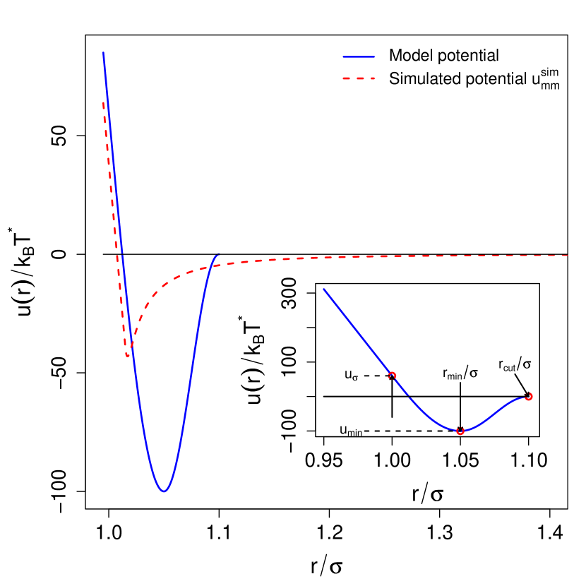
Figure 1: Model and simulated monomer-monomer interaction potentials.

where $u_{\sigma}=u_{mm}^{\textrm{mod}}(\sigma)$, $r_{\textrm{min}}$ is the location of the potential minimum, and $u_{\textrm{min}}=u_{mm}^{\textrm{mod}}(r_{\textrm{min}})$. The model potential depends on five parameters ($r_{\textrm{min}}$, $\sigma$, $r_{\textrm{cut}}$, $u_{\sigma}$, and $u_{\textrm{min}}$) chosen in our numerical simulations as follows. The potential minimum is located at $r_{\rm min}=1.05\sigma$, where it evaluates to $u_{\rm min}=-100k_{B}T$. At monomer separation $\sigma$ the potential evaluates to $u(\sigma)=60k_{B}T$ with a steep gradient. For monomer separations in the range $(0,\sigma]$ the potential is extrapolated linearly with the slope it has at $r=\sigma$. Hence, for separations smaller than $\sigma$, the monomers feel a strong constant repulsive force equal to the force at $r=\sigma$. The cut-off distance is $r_{\textrm{cut}}=1.1\sigma$. The model potential and its various parameters are shown in the inset of Fig. 1.

The interaction potential may be obtained from the integration of the intermolecular interactions over the nanoparticle volumes as in Ref. yannis_potential . We assume pairwise additivity of the intermolecular potential, continuous medium, and constant material properties. Elastic flattening of the monomer is neglected. The intermolecular potential is taken to be the Lennard-Jones potential

$$u_{LJ}(r)=4\epsilon\left[\left(\frac{\sigma_{LJ}}{r}\right)^{12}-\left(\frac{\sigma_{LJ}}{r}\right)^{6}\right]\quad,$$ (11)

where $\epsilon$ is the depth of the attractive potential, the maximum attractive energy between two molecules, and $\sigma_{LJ}$ the distance at which the potential evaluates to zero, the distance of closest approach of two molecules which collide with zero initial relative kinetic energy. The first term expresses (approximately) the repulsive part (Born repulsion), the second the attractive (van der Waals attraction). Integration of Eq. (11) over two equal-sized spheres of diameter $\sigma$ yields, see, for example, Refs. yannis_potential ; ruckenstein , an attractive part

$$u_{mm}^{\textrm{vdW}}(r)=-\frac{A}{6}\ \left[\ln\left(\frac{r^{2}-\sigma^{2}}{r^{2}}\right)+\frac{\sigma^{2}}{2(r^{2}-\sigma^{2})}+\frac{\sigma^{2}}{2r^{2}}\right]\quad,$$ (12a)

and a repulsive part

$$\begin{split}u_{mm}^{\textrm{rep}}(r)={}&\frac{A\sigma_{LJ}^{6}}{2520r}\left\{\sigma^{2}\left[\frac{1}{2(r-\sigma)^{7}}+\frac{1}{2(r+\sigma)^{7}}+\frac{1}{r^{7}}\right]\right.\\ &\left.-\frac{\sigma}{3}\left[\frac{1}{(r-\sigma)^{6}}-\frac{1}{(r+\sigma)^{6}}\right]-\frac{1}{15}\left[\frac{2}{r^{5}}-\frac{1}{(r-\sigma)^{5}}-\frac{1}{(r+\sigma)^{5}}\right]\right\}\quad,\end{split}$$ (12b)

to obtain

$$u_{mm}(r)=u_{mm}^{\textrm{rep}}(r)+u_{mm}^{\textrm{vdW}}(r)\quad,$$ (12c)

where $A=4\pi\epsilon\sigma_{LJ}^{6}n^{2}$ is the Hamaker constant and $n$ the molecular number density in the solid. In the limit $r\gg\sigma$ the potential decays as $u_{mm}\sim-r^{-6}$, i.e., the expected attractive van der Waals interaction energy between two non-charged macroscopic bodies is recovered. The Hamaker constant of a typical soot nanoparticle, for example $n$-hexane, was estimated to be $A=2.38\cdot 10^{-19}$J kasper_hamaker with a corresponding $\sigma_{LJ}=0.5949$nm substance_book . We used these values, along with $\sigma=20$nm, to render the interaction potential dimensionless.

The repulsive part of $u_{mm}$ diverges for $r\to\sigma$; it may, thus, cause numerical difficulties in the solution of the Langevin equations. We modified the potential at distances $r_{\rm mat}=1.015\sigma$ (less than the position of the potential minimum at $r_{\min}\simeq 1.017\sigma$) by extrapolating it linearly with the same slope it has at $r_{\rm mat}$ until $r=0.995\sigma$ (where it evaluates to about $60k_{B}T^{*}$). A similar matching condition was used to determine the coefficient of the model-potential linear term. We set $u_{mm}$ to zero at smaller monomer-monomer separations. This modification of the repulsive part is not expected to affect the dynamics of the system, since it involves monomer separations that are energetically unfavorable (and, hence, unlikely). Therefore, the intermonomer potential we use is

$$u_{mm}^{\textrm{sim}}(r)=0 0\leq r\leq 0.995\sigma\quad,$$ if (13a)

$$u_{mm}^{\textrm{sim}}(r)=\frac{\partial u_{mm}}{\partial r}\bigg{|}_{r_{\rm mat}}(r_{\rm mat}-r)+u_{mm}(r_{\rm mat}) \quad 0.995\sigma<r\leq r_{\rm mat}\quad,$$ if (13b)

$$u_{mm}^{\textrm{sim}}(r)=u_{mm}(r) \quad r_{\rm mat}<r\quad.$$ if (13c)

We truncate the potential at distances $r\geq 7\sigma$ where it is negligible with respect to the thermal energy, $u_{mm}(7\sigma)/(k_{B}T^{*})\sim 10^{-4}$.

Although neither potential diverges at separations $r<\sigma$, at such distances monomers feel a very strong repulsive force; monomer separations below $\sigma$ are energetically unfavorable and their occurrence is extremely unlikely during the system dynamics. This justifies the identification of $\sigma$ with the hard-core monomer diameter. Moreover, since the two intermonomer potentials are much deeper than $k_{B}T^{\star}$ the sticking probability upon collision may be considered to be unity.

In the following, we will use only dimensionless quantities; we will, thus, drop the tilde to simplify notation. Furthermore, unless specified otherwise, the results presented were obtained with $u_{mm}^{\textrm{sim}}$, Eqs. (13). Figure 1 presents and compares the two dimensionless radial potentials.

III Numerical method

III.1 Numerical solver

The numerical simulations were performed with the software package ESPResSo espresso , a versatile package for generic Molecular Dynamics simulations in condensed-matter physics. We used the Molecular Dynamics program with a Langevin thermostat. The Langevin thermostat was construed as formal method to perform Molecular Dynamics simulations in a constant temperature canonical ensemble, see, for example, Ref. Thermostat . It introduces a fictitious viscous force to model the coupling of the system to a thermal bath according to Eqs. (1) that ensures the system temperature fluctuates about the bath mean temperature. The molecular equations of motion with a Langevin thermostat are formally identical to the Langevin equations of interacting Brownian particles: the physical scales and their interpretation differ.

The ESPResSo numerical solver uses the Verlet algorithm for the deterministic part, with a numerical error that scales at least like $O(\delta t^{3})$. The combination of the Verlet algorithm with the solver for the stochastic part (Langevin thermostat) yields an error estimate of $O(\delta t^{3})$ in the monomer positions and of order $O(\delta t^{2})$ in the velocities NumericsEspresso . As a check of the numerical solver we simulated the motion of a single Brownian particle in a quiescent fluid. The simulations for the mean-square displacement $\langle r_{1}^{2}(t)\rangle$, the mean-square velocity fluctuations $\langle v_{1}^{2}(t)\rangle$, and the velocity autocorrelation function $\langle{\bf v}_{1}(t){\bf v}_{1}(0)\rangle$ agreed with the analytical expressions risken_book .

The initial state was created by randomly placing $n_{\infty}(0)V=5000$ monomers in a cubic box of size $L$ with $V=L^{3}$ the box volume, and $n_{\infty}(0)$ the initial monomer concentration. The box size was chosen to give the desired initial monomer concentration according to $L=\left({5000}/{n_{\infty}}\right)^{1/3}$. We chose $n_{\infty}(0)=0.01$ corresponding to $L\simeq 80$. The initial random placement of monomers could cause numerical problems if two or more monomers happen to be placed in almost overlapping positions, thus experiencing immediately a very strong repulsive force. We used a well-known technique of MD simulations to avoid these numerical instabilities by ramping up the repulsive force for $r<1$ to its constant final value during 800 time steps. The (dimensionless) simulation time step was chosen to be $\delta t_{\textrm{sim}}=1.25\times 10^{-3}$. After initialization, the system was evolved until a final time $3000$, when the cluster concentration had decreased by almost two orders of magnitude. The results we show were obtained using the output of $10$ simulations, each one with different initial monomer positions and zero initial monomer velocities. Finally, periodic boundary conditions were imposed.

III.2 Cluster identification

The identification of clusters is one of the most time-consuming tasks of post-processing the simulation results. The ESPResSo simulations return individual monomer positions and velocities. Unlike the previously mentioned works mountain ; meakin_cluster_models , agglomeration events are not identified during the time evolution of the system, but cluster formation is determined a posteriori. Sampling of the simulation output was performed at time intervals $\delta t_{\rm sam}=2$ (every $1,600$ simulation time steps).

We resort to an approach based on graph theory. A cluster is a set of connected, bound, monomers. As both interaction potentials are very deep once two monomers collide and bind, they remain bound: no agglomerate break-up was noticed during our simulations. Hence, two monomers may be considered bound when their relative distance is less than a threshold distance $d_{\rm thr}$. The choice of $d_{\rm thr}$ depends on the position of the minimum of monomer interaction potential $r_{\rm min}$. For the simulations with the integrated Lennard-Jones potential we used $d_{\rm thr}=1.04$, whereas for the model potential we used $d_{\rm thr}=1.06$. Small variations of $d_{\rm thr}$ about these values did not affect the identification of clusters. Our definition of a cluster is reminiscent of the liquid cluster definition proposed by Stillinger and used in gas-liquid nucleation studies (see, for example, Ref. clusterReguera ).

Computationally, the first step is the calculation of the distance matrix ${\bf D}$ between all monomers. For a box with periodic boundary conditions, the distance between two monomers is the distance between the $i$-th monomer and the nearest image of the $j$-th monomer md_book . For instance, the (ordered) distance between two monomers along coordinate $l$ is

$$D_{ij}^{l}=r_{i}^{l}-r_{j}^{l}-L\cdot{\rm nint}\left(\frac{r_{i}^{l}-r_{j}^{l}}{L}\right)\quad,\quad l=x,y,z\quad,$$ (14)

where “nint” is the nearest integer function. The periodicity of the box imposes a cut-off of $L/2$ on the maximum distance between two monomers along each axis. The three-dimensional distance

$$D_{ij}=\Big{[}\sum_{l=1}^{3}\big{(}D_{ij}^{l}\big{)}^{2}\Big{]}^{1/2}\quad,$$ (15)

is always a non-negative quantity. The distance matrix $\bf{D}$ is subsequently used to calculate the adjacency matrix $\bf{A}$, defined as

$$A_{ij}=\begin{cases}1&\quad\text{if }\quad D_{ij}\leq d_{\rm thr}\quad,\\ 0&\quad\text{otherwise}\quad.\end{cases}$$ (16)

The adjacency matrix is usually introduced in graph theory book_algorithms as a convenient way to represent a graph uniquely. Monomers in a cluster can be formally regarded as graph vertices (nodes), whereas the bonds due to the interaction potential become graph edges (links). The problem of cluster identification, given the distance matrix ${\bf D}$, is then re-formulated as the identification of the connected components of a non-directed graph expressed by the (symmetric) adjacency matrix ${\bf A}$. They can be determined using a standard breadth-first search algorithm book_algorithms . Due to its speed and scalability, we resort to the implementation of its algorithm in the igraph library igraph .

III.3 Cluster radius of gyration

The radius of gyration is a geometric parameter used to characterize the size of fractal aggregates. It describes the spatial mass distribution about the aggregate center of mass. As such it is a static property that depends on the cluster mass distribution, and not on the diffusive properties of the cluster. For a cluster composed of $k$ equal-mass monomers it becomes the root-mean-square distance of the monomers from the cluster center of mass Filippov et al. (2000)

$$R_{g}^{2}=\frac{1}{k}\,\sum_{i=1}^{k}{({\bf r}_{i}-{\bf R}_{CM})^{2}}+a_{1}^{2}\quad,$$ (17a)

where the aggregate center of mass is

$${\bf R}_{CM}=\frac{1}{k}\,\sum_{i=1}^{k}{\bf r}_{i}\quad,$$ (17b)

and $a_{1}$ a monomer characteristic size. Since we are interested in the power-law dependence of the radius of gyration on the number of monomers in a cluster even for small clusters we included $a_{1}$ in the definition of the radius of gyration: otherwise Eq. (17a) evaluates to zero for a monomer. The additional term may be taken to be either the primary particle radius Filippov et al. (2000), $a_{1}=\sigma/2$, or the radius of gyration of a sphere sorensen_prefactor , $a_{1}=\sqrt{3/5}(\sigma/2)$. The choice of $a_{1}$ as the monomer radius of gyration ensures that, if an average fractal exponent is used, the large $k$ behaviour in the power-law scaling persists even for smaller clusters. Of course, the value of $a_{1}$ (including $a_{1}=0$) is irrelevant for large clusters. We used both choices for $a_{1}$: the results presented were obtained with $a_{1}$ the monomer radius of gyration because this choice gave better agreement of the calculated and numerically estimated kernel elements, see Sec. V.5. Nevertheless, the difference between the two choices was small.

The calculation of $R_{g}$ according to Eq. (17a) must take into consideration the periodicity of the box. Since all monomer-monomer distances are known from Eq. (14), the position of monomers in the cluster with respect to a randomly selected monomer (say monomer $1$) may be easily calculated; for instance, the $j$-th monomer position along coordinate $l$ with respect to monomer $1$ is

$$r_{j}^{l}=r_{1}^{l}+D_{1j}^{l}\quad\quad.$$ (18)

Given the relative position of all monomers in the cluster, the position of the aggregate center of mass may be calculated via Eq. (17b), and the radius of gyration from Eq. (17a). We adopted a reference system centered on the randomly chosen monomer in the cluster, i.e., ${\bf r}_{1}=(0,0,0)$. For this reference system $r_{j}^{l}=D_{1j}^{l}$. This procedure is independent of the choice of the selected monomer, since the radius of gyration is independent of the cluster position in the box, nor does the procedure depend on the sign convention chosen for $D_{1j}^{l}$.

III.4 Collision kernel

The package ESPResSo allows addressing each monomer individually at all times during the simulation, i.e. a permanent label (e.g., color) may be associated with each monomer. A monomer label allows the unequivocal identification of the cluster it belong to. Each cluster becomes an unordered collection of monomer labels where no monomer label is repeated: this amounts to the mathematical definition of a set. Viewing clusters as sets of monomer labels provides a computational method to investigate cluster collisions even for sampling times considerably longer than the simulation time step, as long as the aggregates do not break-up. To be specific, consider two clusters at time $t$. If during the (sampling) time interval $(t,t+\delta t_{\textrm{sam}}]$ they collide, they will be part of the same newly-formed cluster at $t+\delta t_{\textrm{sam}}$. An equivalent description of the collision is that the two monomer-label sets that identify the pre-collision clusters become proper subsets of the monomer-label set that identifies the cluster formed by their collision, and detectable at $t+\delta t_{\textrm{sam}}$. The number of collisions that occurred during $(t,t+\delta t_{\textrm{sam}}]$, and the clusters involved in the collisions, may be recorded simply by comparing different sets.

The collision kernel $K_{ij}$ (rendered dimensionless by scaling it by $\sigma^{3}/\tau_{1}$) between an $i$-mer and $j$-mer during the sampling time interval is

$$\frac{N_{ij}(t)}{V\delta t_{\textrm{sam}}}=(2-\delta_{ij})K_{ij}\frac{N_{i}(t)}{V}\frac{N_{j}(t)-\delta_{ij}}{V}\cong(2-\delta_{ij})K_{ij}n_{i}(t)n_{j}(t)\quad,$$ (19)

where $N_{ij}(t)$ is the number of collisions between $i$- and $j$-mers that took place during the interval $(t,t+\delta t_{\textrm{sam}}]$, $N_{i}(t)$ is the number of $i$-mers at time $t$, $n_{i}(t)=N_{i}(t)/V$ the cluster concentration, and $\delta_{ij}$ the Kroenecker delta. The collision kernel $K_{ij}$ is estimated from Eq. (19) by treating it as the fitting parameter that minimizes (in a least-square sense) the distance between the number of detected collisions $N_{ij}(t)/(V\delta t_{\textrm{sam}})$ and $(2-\delta_{ij})K_{ij}n_{i}(t)n_{j}(t)$.

IV Static cluster properties

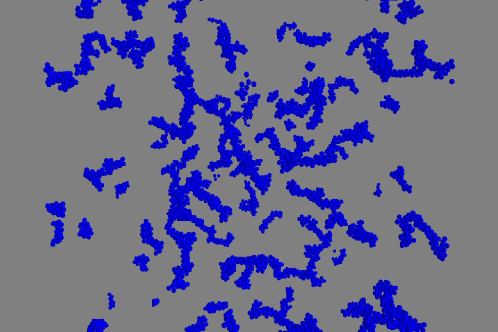
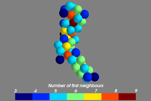
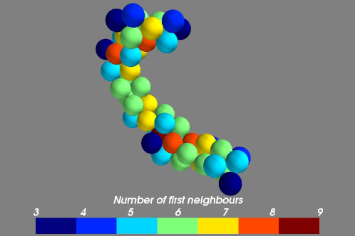
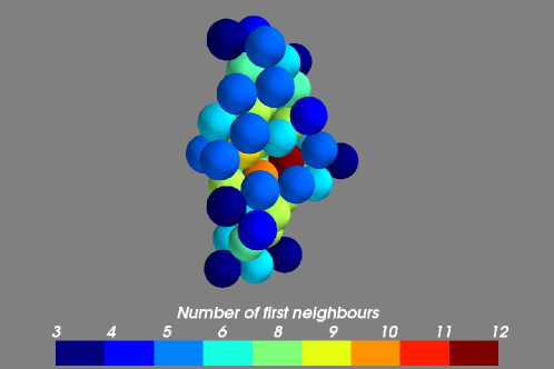
Figure 2: Clockwise from top: Snapshot of the system at the end of a simulation ($t_{\textrm{final}}=3000$) followed by three different $50$-monomer aggregates. Three dimensional images created with the software Mayavi2 mayavi2 . The color code denotes number of first monomer neighbours.

Examples of 50-monomer clusters that survive at the end of one of the simulations are shown in Fig. 2. The top, left subfigure is a snapshot of the system, whereas the other three are color-coded aggregates. The color code denotes the number of first neighbours of a monomer. Note the relatively compact and long, tubular structure of the generated aggregates. These two features, small-scale compactness and large-scale tubular structure, will be related to properties of the intermonomer potential in the following sections.

IV.1 Cluster fractal dimension

The fractal dimension of the clusters is determined from the statistical scaling law that governs the power-law dependence of the cluster radius gyration $R_{g}$ on cluster size $k$

$$R_{g}=ak^{1/d_{f}}\quad,$$ (20)

where $d_{f}$ is the average, time-independent fractal dimension of the aggregates, and $a$ the fractal prefactor, occasionally referred to as lacunarity Rosner95 . The fractal prefactor provides information on the packing of monomers WuFriedlander93 . The cluster radius of gyration was obtained by averaging over generated cluster configurations. Specifically, the average radius of gyration of a $k$-monomer aggregate is taken over all $k$-monomer aggregates that had been recorded at least $200$ times. This requirement aims at eliminating outliers. It is not particularly stringent since for each simulation $1500$ system configurations (snapshots) were stored, and $10$ simulations. Our results are not sensitive to reasonable choices of the threshold of minimum number of cluster occurrences: raising the occurrence threshold to $400$ does not change the calculated fractal dimension.

Figure 3 presents the calculated radius of gyration as a function of aggregate size. The double logarithmic plot shows that power-law scaling breaks down for cluster sizes $k<5$. Hence, we set $k=5$ the minimum cluster size in the fits. All cluster configurations with $k\geq 5$ were fitted to a single line leading to an average fractal exponent $d_{f}=1.62\pm 0.02$, and a prefactor $a=0.242\pm 0.006$. The prefactor re-expressed in terms of $k=k_{g}(2R_{g})^{d_{f}}$ gives $k_{g}=3.24$. The calculated prefactor is on the high side of fractal prefactors reported in the literature for clusters generated by computer simulations PrefactorAeroSci00 , but closer to experimentally determined prefactors that indicate $k_{g}>2$  PrefactorAeroSci00 ; Rosner95 . Inspection of the figure shows that clusters with $k\leq 15$ deviate significantly from the single-line fit. Simulation results are fitted better by considering two cluster population (and hence two different slopes): we identify small ($k\leq 15$) and large ($k>15$) clusters. Refitting the data gives a fractal dimension $d_{f}^{mc}=2.25\pm 0.05$ for small clusters and $d_{f}^{cc}=1.56\pm 0.02$ for large clusters. The corresponding average prefactors, as well as the fractal dimensions, are reported in Table 1. As before, the prefactor for the large clusters are on the high side of literature-reported values for computer-generated clusters, and closer to experimental values determined by angular light scattering, suggesting that the cluster generated in this study have a closely packed structure WuFriedlander93 , see also Fig. 2.

The presence of two cluster populations obeying scaling laws with different exponents may be attributed to different agglomeration mechanisms. Small clusters are generated mainly by monomer-cluster agglomeration; they are more compact and spherical than large clusters. This agglomeration process is similar to, but different from, diffusion-limited aggregation, as argued in Sec. IV.2. Large clusters are mainly generated by cluster-cluster agglomeration. Therefore, it is expected, and numerically confirmed, that $d_{f}^{mc}>d_{f}^{cc}$. Furthermore, the calculated fractal dimension of large clusters is comparable, but lower, to reported fractal dimensions of cluster-cluster agglomeration $d_{f}\sim 1.7-1.8$ mountain ; smirnov_review . Further comments on the agglomeration process and the associated fractal dimensions are made in Sec. IV.2.

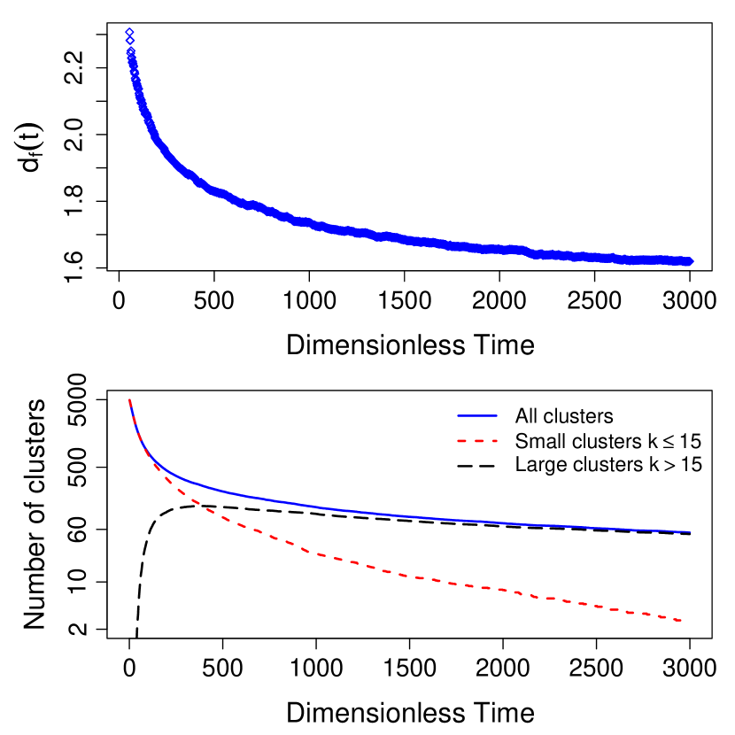
Figure 4: Top: Aggregate fractal dimension as a function of time. Bottom: Total number of clusters (solid), number of small clusters $k\leq 15$ (short dashed), and number of large clusters $k>15$ (long dashed).

The existence of two cluster populations that arise from the predominance of different agglomeration mechanisms as agglomeration progresses suggests the calculation of a time-dependent average fractal dimension $d_{f}(t)$. We calculated it by considering the instantaneous radius of gyration of $k$-monomer clusters for each of the ten initial configurations: only clusters with $k\geq 5$ were included, and no occurrence threshold was imposed. As the number of clusters is considerably smaller than those used in the time-independent calculation we do not calculate first the instantaneous average radius of gyration and then fit the data (as done for the calculation presented in Fig. 3): instead we fit all the data simultaneously (no averaging). The fractal dimension as a function of time is shown in Fig. 4 (top). The evolution of the fractal dimension may be linked to the kinetics of the small and large cluster populations. At early times, the system is almost entirely made up of small clusters ($k\leq 15$), Fig. 4 (bottom), hence $d_{f}(t)\simeq d_{f}^{mc}$, whereas at late times the contribution of large clusters ($k>15$) to the overall cluster population is dominant, hence $d_{f}(t)\to d_{f}^{cc}$.

These findings are in the spirit of the study by Kostoglou and Konstandopoulos konstandopoulos who used a distribution of fractal dimensions to characterize aggregate morphology. They showed that the mean fractal dimension relaxes to an a priori fixed asymptotic value specified by the dominant agglomeration mechanism. Our results on the importance of agglomeration kinetics on the evolution of $d_{f}(t)$ are in agreement with earlier works, e.g., Refs. mountain ; smirnov_review who suggest that the aggregate fractal dimension depends mainly on the dominant agglomeration mechanism.

IV.2 Cluster morphology

As a measure of local compactness of the generated aggregates we calculated the cluster coordination number. The cluster coordination number, defined as the mean number of first neighbours of a monomer in a cluster, provides information on the openness of the aggregates and their compactness, and on the presence of cavities in their structure, i.e., their porosity. Hence, it is related to the fractal prefactor, Eq. (20); it characterizes the small-scale structure of an aggregate, whereas the fractal dimension characterizes its large-scale structure. The coordination number varies between 0 and 12 for spherical particles, reaching its highest value for hexagonal close packed (hcp) or face centered cubic (fcc) structures at a volume fraction of 0.74 Hutter . The cluster coordination number is obtained during post-processing of the simulation results resorting again to the igraph library igraph .

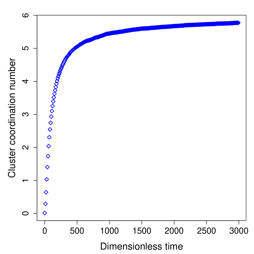
Figure 5: Mean cluster coordination number.

We calculated the mean cluster coordination number by averaging the coordination number of each cluster over all clusters at a given time. It is plotted in Fig. 5 as a function of time. At late times it reaches values higher than five, implying that the aggregates are relatively compact.

The local, small-scale compactness of the aggregates, aggregates that are similar to those generated by the Langevin simulations of, e.g, Ref. videcoq , is related to the spherical symmetry of the monomer-monomer interaction potential. At early times when a monomer collides and binds to an aggregate it is free to slide, a motion induced by the thermal noise, and to reorient to maximize the number of contacts with other monomers. Since the potential is isotropic there is no angular restoring force to prevent sliding. However, short-time restructuring is hindered as the number of monomer-monomer contact points increase because the energy cost associated with stretching monomer-monomer bonds is high. Inspection of Fig. 2 shows that the minimum number of first neighrours in a stable cluster is three, suggesting that in three dimensions three contact points are sufficient to prevent monomer sliding. Hence, the aggregates generated herein are different from those generated by diffusion-limited aggregation where colliding monomers remain fixed at the initial point of contact. Becker and Briesen TangentialForces showed that in the absence of a potential to prevent bending of monomer-monomer bonds the aggregate collapses to a more compact structure. The monomer reorientation at early times also suggests that the high fractal dimension $d_{f}^{mc}$ we associated with monomer-cluster agglomeration mechanism arises from monomer rearrangement. In our simulations monomer reorientation occurred at very small time scales, smaller than the sampling time. After the short-time monomer reorientation clusters remain rigid till the next collision, as discussed Sec. IV.3.

An additional explanation for the compactness of aggregates generated by Langevin simulations, neglecting Brownian motion, was suggested by Tanaka and Araki prl_hydro . They argued that in the absence of interparticle hydrodynamic interactions, in particular of squeezed-flow effects, the generated clusters tend to be more compact.

Even though the clusters are locally compact, the large clusters generated at late times have a low fractal dimension $d_{f}^{cc}<2$. Inspection of Fig. 2 (second and third clusters) suggests that the low, late-time fractal dimension is due to their tubular, elongated shape. The aggregates are not porous: they do not have holes nor cavities. The large-scale structure of the late-time (large) clusters is determined by the attractive range of the intermonomer potential. At late times when two (locally compact) clusters collide aggregate restructuring is limited to the monomers that are in contact: the attractive range of the potentials used in the simulation is too short to induce significant cluster re-organization, a process that would increase the fractal dimension. Videcoq et al. videcoq showed that increasing the attractive range modifies the shape of the generated aggregates leading to more spherical aggregates. Hence, the late-time fractal dimension associated with cluster-cluster aggregation depends on the extend of restructuring due to the attractive potential range. This restructuring provides a possible explanation of the lower than expected fractal dimension for cluster-cluster aggregation.

Additional simulations were performed to assess the sensitivity of the observed cluster morphology, and their rigidity, on the simulation time step. We simulated a $50$-monomer cluster (shown at the bottom right, Fig. 2) for $32000$ time steps ($t_{\textrm{final}}=40$), with two different time steps, $\delta t_{\textrm{sim}}$ and $\delta t_{\textrm{sim}}/4$. We monitored the time evolution of the cluster radius of gyration $R_{g}(t)$, an average cluster property, and an instantaneous cluster property, the distance $d_{1,12}(t)$ of two randomly chosen monomers (monomers $1$ and $12$). We found that both quantities fluctuated by approximately $0.1\%$, independently of time step. These results confirm that cluster morphology does not depend on the choice of the time step, as long as it is chosen within reason. In fact, for considerably longer time steps the cluster breaks up. The fluctuations arise because monomer radial positions fluctuate, albeit slightly, about the potential minima.

As a different measure of a possible dependence of cluster morphology on the simulation time step we compared the time-dependent adjacency matrices, Eq. (16), for these two simulations. The adjacency matrices were found to be all identical, another confirmation that cluster morphology is independent of the time step. Note that small fluctuations of monomer radial positions in the cluster are not reflected in the adjacency matrix (a binary matrix) since a distance threshold is used to convert the distance matrix, Eq. (15), to it.

Thus, the morphology of the generated aggregates arises from a combination of kinetic effects, as induced by the thermal noise, and energetic effects, as determined by the attractive range of the interaction potential. A precise characterization of aggregate morphology requires both the fractal dimension and the coordination number (or the lacunarity).

IV.3 Cluster restructuring

In addition to short-time monomer reorientation cluster restructuring may occur following a cluster-cluster collision. Cluster restructuring following contact of two clusters was investigated in a three-dimensional lattice model in Ref. meakin_reorganization_3D . In our approach cluster restructuring does not have to be imposed as an additional feature of cluster dynamics, but it occurs naturally. The deep radial intermonomer potential locks distances between neighbouring monomers, but bonded monomers may slide over each other due to the thermal noise term. However, as mentioned earlier, monomer sliding is restricted by the number of monomer-monomer contact points.

We use two statistical quantities as indicators of the modification of the structure of a cluster: the radius of gyration and the mean monomer-monomer distance. For a $k$-mer the mean monomer-monomer distance $D_{mm}$ is the average monomer-monomer distance over all the monomers,

$$D_{mm}=\frac{1}{k^{2}}\,\sum_{i,j}^{k}D_{ij}\quad,$$ (21)

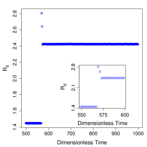
Figure 6: Top: Mean monomer-monomer distance of a selected cluster. Bottom: Radius of gyration of the same cluster.

where the monomer-monomer distance $D_{ij}$ was defined in Eq. (15). We monitored cluster restructuring by selecting a monomer at the beginning of the simulation and follow it as it collides with other monomers or clusters. In Fig. 6 (left) we show $D_{mm}$ during a period when a collision occurs ($t=568$) and the cluster size increases from $k=14$ to $k=43$ . We notice that before and after the collision $D_{mm}$ is constant, a clear sign of cluster rigidity. When the collision between the two aggregates occurs, $D_{mm}$ increases, but on a time scale of a few monomer relaxation times it decreases, afterwards remaining relatively constant. We consider this behaviour a strong indication of cluster reorganization following the collision of two clusters. The cluster radius of gyration shows a perfectly analogue behavior, Fig. 6 (right). Note, however, that once cluster restructuring occurs after a cluster-cluster collision the resulting cluster retains its shape and it remains rigid until possibly the next collision.

V Dynamic cluster properties

V.1 Cluster translational diffusion coefficient

Equations (1) determine the dynamics of each monomer and indirectly the cluster diffusive properties. The cluster diffusion coefficient is calculated from the late-time dependence of the variance of the cluster center-of-mass position as a function of time risken_book

$$\langle\delta{R}^{2}_{CM}(t)\rangle=\langle\big{[}{\bf R}_{CM}(t)-\langle{\bf R}_{CM}(t)\rangle\big{]}^{2}\rangle\ \xrightarrow{t\to\infty}6D_{k}t\quad.$$ (22)

A different set of simulations was performed to determine the diffusion coefficient of a few selected clusters. As noted in Sec. IV.3 in the absence of collisions clusters are rigid: the dynamical properties presented in this section refer to perfectly rigid clusters. A selected cluster was placed in the simulation box with its centre-of-mass position at ${\bf R}_{CM}=(0,0,0)$ and with zero monomer velocities. The box size was chosen to be $L=10,000$, a size much larger than the box size used for the agglomeration simulations. A large box is necessary because the aggregate centre of mass has to be tracked for a (potentially) long time, and, due to the periodic boundary conditions, no displacement of the aggregate from its initial position larger than $L/2$ is admissible. For these simulations the cluster never crossed the boundary of the box.

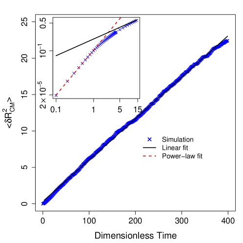
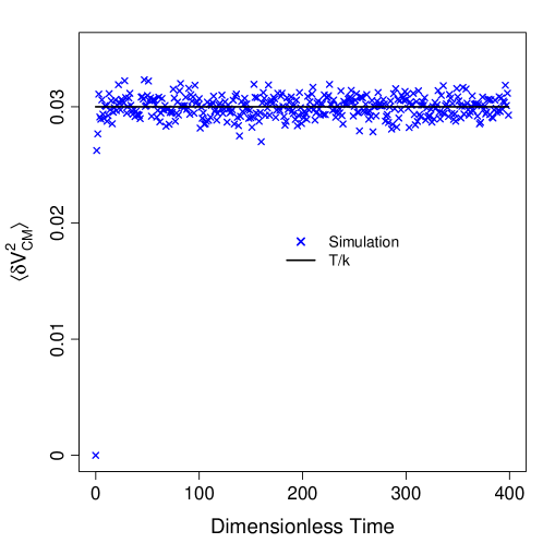
Figure 7: Top: Mean-square cluster displacement averaged over 800 trajectories (crosses) and linear fit (solid line) of a $50$-monomer cluster (shown in Fig. 2, bottom right). Inset: Early-time behaviour of $\langle\delta R^{2}_{CM}\rangle$ (crosses), linear fit (solid line) and power-law fit, $\gamma=3$ (dashed line). Bottom: Velocity fluctuations $\langle\delta V^{2}_{CM}\rangle$ (crosses) and analytical expression, Eq. (28) (solid line).

The center of mass of a single cluster was tracked up to $t=400$ for clusters with $k=4,10,50,98$. Averages were performed over $800$ trajectories, each trajectory starting with an identical cluster: different cluster trajectories arise from different realizations of the stochastic noise. Figure 7 (top) shows $\langle\delta{R}^{2}_{CM}(t)\rangle$ for a $50$-monomer cluster, chosen to be the cluster at the bottom right of Fig. 2. The time dependence of the ensemble-averaged, mean-square cluster displacement quickly becomes linear, in agreement with Eq. (22). The inset of Fig. 7 (top) magnifies (on a double logarithmic scale) the early-time behavior of $\langle\delta{R}^{2}_{CM}(t)\rangle$. For $t\leq 1$ cluster motion is ballistic, and the mean-square displacement exhibits a power-law dependence on time, $\langle\delta{R}^{2}_{CM}(t)\rangle\propto t^{\gamma}$ with $\gamma=3$. This is the expected behaviour for a single Brownian monomer with zero initial velocity risken_book . Similar early-time ballistic motion was found for a cluster with $k=4$.

The results of the numerical simulations for the four clusters are summarized in Table 2, where we also report the cluster radius of gyration (obtained from Fig. 3). They may be interpreted by considering theoretical estimates of the diffusion coefficient $D_{k}$ of a $k$-mer. The Stokes-Einstein diffusion coefficient of a single spherical monomer, in dimensionless form, scaled by $D^{\star}=k_{B}T^{\star}/(\beta_{1}m_{1})$, is risken_book

$$D_{1}=T\quad.$$ (23)

The diffusion coefficient of a $k$-mer of mass $M_{k}=km_{1}$ may be expressed as a generalization of Eq. (23). Let $\beta_{k}$ be the average friction coefficient of a monomer in the $k$-cluster. Then, the cluster drag term in Eq. (1) may be written as $\beta_{k}M_{k}=k\beta_{k}m_{1}$, and the cluster diffusion coefficient generalizes to

$$D_{k}=D_{1}\,\frac{\beta_{1}}{k\beta_{k}}\equiv D_{1}\,\frac{1}{k\eta_{k}}\quad.$$ (24)

Equation (24) manifestly shows the importance of the ratio of the average friction coefficients $\eta_{k}=\beta_{k}/\beta_{1}$, $\eta_{k}$ being the average shielding factor of a monomer in a $k$-cluster. In fact, Filippov et al. (2000), in a different context, used the cluster shielding factor to describe how monomer shielding affects heat transfer to an aggregate. Herein, the cluster shielding factor is connected to cluster mobility.

The numerically determined diffusion coefficients behave as $D_{k}\propto 1/k$ with $k$ spanning almost two orders of magnitude. The estimated value of $\beta_{k}$ equals the monomer friction coefficient $\beta_{1}$ within a few percents, Table 2 ($\beta_{1}=1$ in our units). The small deviations are attributable to the limited number of simulated stochastic trajectories. Our Langevin simulations suggest that the cluster diffusion coefficient is inversely proportional to the cluster mass and to the monomer friction coefficient. This behaviour is a direct consequence of neglecting shielding of inner monomer by outer monomers in an aggregate. The cluster accessible area becomes the sum of the monomer accessible areas, since for $\eta_{k}=1$ the total friction coefficient of a $k$-mer is $3\pi\mu_{f}\sigma k$. For this reason we refer to these clusters as ideal clusters, with respect to their dynamical properties. For ideal clusters the average monomer shielding factor is unity irrespective of the state of aggregation of the monomer. This is an inherent property of all simulations of monomer agglomeration via the unshielded monomer Langevin equations Eqs. (1).

The cluster diffusion coefficient (in the continuum regime) is frequently expressed in terms of a mobility radius $R_{m}$, the radius of a sphere with the same friction coefficient as the aggregate friedlander book . In the dimensionless units used in this work, the mobility radius determines the cluster diffusion coefficient by

$$D_{k}=D_{1}\,\frac{1}{2R_{m}}\quad.$$ (25)

Comparison of Eqs. (24) and (25) gives an expression for the mobility radius in terms of the (average) cluster (per-unit-mass) friction coefficients $\beta_{k}$ and $\beta_{1}$, or the shielding factor $\eta_{k}$,

$$R_{m}=\frac{k}{2}\,\frac{\beta_{k}}{\beta_{1}}=\frac{k}{2}\,\eta_{k}\quad.$$ (26)

For the ideal clusters generated in this work $R_{m}=k/2$. Table 2 presents the mobility radius calculated either from the numerically determined diffusion coefficient [Eq. (25), fourth row], or by evaluating it directly from Eq. (26) with $\eta_{k}=1$ (fifth row). A comparison of these two values provides an indication of the numerical error of our simulations: the percentage shown in the fifth row (in parenthesis) quantifies the difference.

The cluster diffusion coefficient is frequently estimated by taking the aggregate mobility radius $R_{m}$ approximately equal to the cluster radius of gyration $R_{g}$. Our simulations show that the radius of gyration is of the same order of magnitude for cluster sizes in the range $k=4$ to $k=98$, whereas the mobility radius is considerably higher. Since the radius of gyration severely underestimates the mobility radius, the diffusion coefficient of ideal clusters is lower than the diffusion coefficient of clusters with $R_{m}\sim R_{g}$. In ideal clusters the average monomer shielding factor is unity, whereas monomers in non-ideal clusters are at least partially shielded, resulting in higher cluster mobility, cf. Eq. (24).

V.2 Cluster thermalization

For a single Brownian monomer, the late-time mean-square velocity fluctuations (dimensionless, scaled by $k_{B}T^{\star}/m_{1}$) tend to risken_book

$$\langle\delta v_{1,\infty}^{2}\rangle=\lim_{t\rightarrow\infty}\langle\big{[}{\bf v}_{1}(t)-\langle{\bf v}_{1}(t)\rangle\big{]}^{2}\rangle=T\quad,$$ (27)

where ${\bf v}_{1}(t)$ is the monomer instantaneous velocity. For a $k$-mer the previous expression, a manifestation of energy equipartition and a consequence of the FDT, may be generalized to

$$\langle\delta V_{CM,\infty}^{2}\rangle=\lim_{t\rightarrow\infty}\langle\big{[}{\bf V}_{CM}(t)-\langle{\bf V}_{CM}(t)\rangle\big{]}^{2}\rangle=\langle\delta v_{1,\infty}^{2}\rangle\,\frac{1}{k}\quad,$$ (28)

where the cluster centre-of-mass velocity is ${\bf V}_{CM}(t)=\sum_{i}{\bf v}_{i}/k$, with ${\bf v}_{i}$ the $i$-th monomer velocity. As for a Brownian monomer Eq. (28) expresses energy equipartition for a $k$-monomer cluster. In Fig. 7 (bottom) we plot $\langle\delta V_{CM}^{2}(t)\rangle$ as a function of time for the 50-monomer cluster used in the previous section. As shown, Fig. 7 (bottom), $\langle\delta V_{CM,\infty}^{2}(t)\rangle$ tends at late times to $0.03$ (up to noise fluctuations), i.e., the theoretical value for ideal clusters, Eq. (28), for the simulation parameters $T=0.5$ and $k=50$.

The main result of Secs. V.1 and V.2 is that a monomer in an ideal $k$-cluster generated according to Eqs. (1) and (2), i.e., neglecting monomer shielding, feels the same friction coefficient as an isolated monomer ($\beta_{k}=\beta_{1}$). An ideal $k$-monomer aggregate has the same diffusive properties as a monomer sphere of $k$ times the mass of a single monomer ($D_{k}=D_{1}/k$). The cluster diffusion coefficient differs from the monomer diffusion coefficient only due to the larger cluster mass, and not, in addition, due to the decrease of the average monomer shielding factor.

V.3 Cluster rotation

We investigated whether ideal clusters have a preferential orientation by examining the distributions of their average Euler angles. As argued, clusters in the absence of collisions may be treated as rigid bodies. Rigid body rotation in three dimensions may be described by the three Euler angles $\theta$, $\phi$ and $\psi$ Goldstein (1950). We evaluated them during post-processing by eliminating cluster translational motion via rigidly translating the cluster centre of mass to the origin of the computational-box coordinate system at all times. The Euler angles may, then, be calculated by recording the time-dependent positions ${\bf r}_{A}(t)$, ${\bf r}_{B}(t)$ and ${\bf r}_{C}(t)$ of three non-coplanar monomers. We define a 3 by 3 matrix ${\bf X}(0)=[{\bf r}_{A}(0),{\bf r}_{B}(0),{\bf r}_{C}(0)]$ containing the initial positions of the three reference monomers and a matrix ${\bf X}^{\prime}(t)=[{\bf r}_{A}(t),{\bf r}_{B}(t),{\bf r}_{C}(t)]$ with their positions at time $t$. The rotation matrix ${\bf A}$ such that ${\bf X}^{\prime}={\bf AX}$ is

$${\bf A}(t)={\bf X}^{\prime}(t){\bf X}^{\textrm{T}}(0)\,\Big{[}{\bf X}(0){\bf X}^{\textrm{T}}(0)\Big{]}^{-1}\quad,$$ (29)

where the superscript T denotes matrix transpose. Once the rotation matrix $\bf A$ is known, the Euler angles may be determined. Since they are not uniquely defined, their values depending on the order of the three rotations, we chose to calculate them via the algorithm presented in Ref. rotation_alghoritm . The range of the Euler angles so determined is: $\phi$ and $\psi$ range in the interval $[-\pi,\pi]$, whereas $\theta$ lies in the interval $[-\pi/2,\pi/2]$. For uniform random rotation matrices random_euler , both $\psi$ and $\phi$ are random variables with a uniform probability distribution in the interval $[-\pi,\pi]$: hence $\langle\phi\rangle=\langle\psi\rangle=0$ and $\langle\delta\phi^{2}(t)\rangle^{1/2}=\langle[\phi(t)-\langle\phi(t)\rangle]^{2}\rangle^{1/2}=\langle\delta\psi^{2}(t)\rangle^{1/2}={\pi}/{\sqrt{3}}\simeq 1.81$. On the other hand, the Euler angle $\theta$ is distributed according to random_euler

$$\theta=\arccos(1-2Z(0,1))-\frac{\pi}{2}\quad,$$ (30)

where $Z(0,1)$ is a random variable with a uniform probability distribution in the interval $[0,1]$. The corresponding averages, obtained numerically, are $\langle\theta(t)\rangle=0$ and $\langle\delta\theta^{2}(t)\rangle^{1/2}\simeq 0.68$.

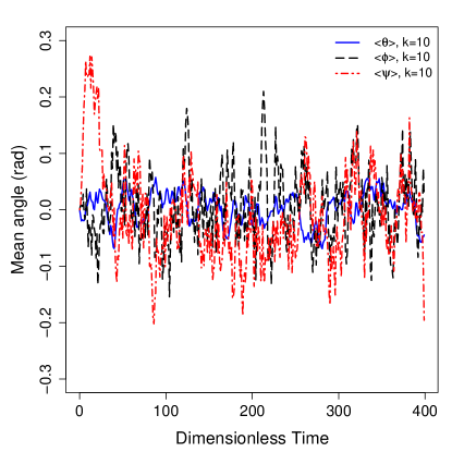
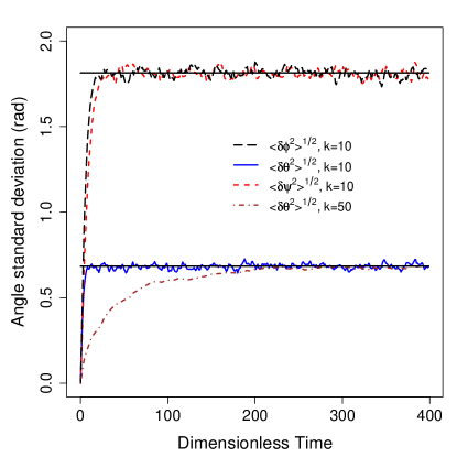
Figure 8: Top: Mean Euler angles $\langle\theta\rangle$ (solid line), $\langle\phi\rangle$ (dashed line) and $\langle\psi\rangle$ (dot-dashed line), averaged over 800 trajectories, for a $10$-monomer cluster. Bottom: Standard deviations $\langle\delta\theta^{2}\rangle^{1/2}$ (solid line), $\langle\delta\phi^{2}\rangle^{1/2}$ (long-dashed line), and $\langle\delta\psi^{2}\rangle^{1/2}$ (short-dashed line) for the same $10$-monomer cluster, and $\langle\delta\theta^{2}\rangle^{1/2}$ (dot-dashed line) for a $50$-monomer cluster. The horizontal lines are the standard deviations of random rotation matrices.

Figure 8 (top) shows the mean Euler angles calculated for an ensemble of $800$ identical clusters containing $10$ monomers each. Their mean values fluctuate about zero. On the bottom diagram we show their mean-square fluctuations: they rapidly tend to the expected values for random rotation matrices. Another calculation of $\langle\delta\theta^{2}\rangle$ for an ensemble of $800$ identical cluster with $k=50$ shows saturation to the same value but on a longer time scale. The rotational thermalization time of an ideal $k$-cluster depends on its total mass. Hence, at late times an ideal cluster does not have a preferential orientation.

V.4 Time dependence of cluster number: The agglomeration equation

The instantaneous total number of clusters, $N_{\infty}(t)=\sum_{k}^{\infty}N_{k}(t)$, quantifies the progress of agglomeration. It may be calculated via the numerical solution of the agglomeration equation friedlander book

$$\frac{dn_{k}}{dt}=\frac{1}{2}\sum_{i+j=k}K_{ij}n_{i}n_{j}-n_{k}\sum_{i}K_{ik}n_{i}\quad.$$ (31)

For definitions and scalings see Section III.4. In this section the collision kernel $K_{ij}$ is scaled by $K^{\star}=D^{\star}\sigma=\beta_{1}\sigma^{3}$, see Eq. (6).

The standard treatment of the collision kernel for fractal aggregates in the continuum regime gives friedlander book

$$K_{ij}=4\pi(D_{i}+D_{j})(R_{i}+R_{j})\quad,$$ (32)

where we dropped the subscript $g$ in the radius of gyration of an $i$-mer, $R_{i}=R_{g,i}$, to simplify notation. Equation (32) is often expressed in terms of the aggregate volume of solids $\nu_{i}\propto(R_{i})^{d_{f}}$ LorenzoJAS since the volume of solids is conserved during agglomeration. Moreover, the diffusion coefficients in Eq. (32) are given by Eq. (25) with the mobility radius being the radius of gyration. The kernel then reads

$$K_{ij}^{Sm}=2\,\pi\,D_{1}\,\left(\frac{1}{\nu_{i}^{1/d_{f}}}+\frac{1}{\nu_{j}^{1/d_{f}}}\right)\,\left(\nu_{i}^{1/d_{f}}+\nu_{j}^{1/d_{f}}\right)\,,$$ (33)

where the superscript $Sm$ refers to the so-called Smoluchowski kernel. The Smoluchowski kernel is not expected to model our numerical results accurately because it is based on diffusion coefficients given by Eq. (25) with $R_{m}=R_{g}$, an equality not respected by our simulations. Instead, the numerical simulations may be used to derive a modified kernel appropriate for the reproduction of the numerical results. Such a kernel is obtained by using the numerically determined cluster diffusion coefficients, Eq. (24) with $\beta_{k}=\beta_{1}$ in Eq. (32) For the radius of gyration, we use the fitted value for $k\geq 5$ (and the data reported in Table 1) to obtain

$$R_{i}=\begin{cases}\textrm{simulation data},&i<5\quad,\\ a_{mc}\,i^{1/d_{f}^{mc}},&5\leq i\leq 15\quad,\\ a_{cc}\,i^{1/d_{f}^{cc}},&15<i\quad.\\ \end{cases}$$ (34)

Furthermore, non-continuum effects arising from monomer-monomer collisions, and dependent on the monomer mean free path, have been shown to be important in combustion-generated nanoparticle agglomeration LorenzoJAS . They may be accounted for by introducing the (dimensionless) Fuchs correction factor $\beta_{F}$ in the kernel: for the explicit expression of $\beta_{F}$ consult Ref. LorenzoJAS . Hence, the kernel appropriate for the Langevin simulations (hereafter referred to as Langevin-Dynamics kernel) reads

$$K_{ij}^{LD}=4\,\pi\,D_{1}\,\left(\frac{1}{i}+\frac{1}{j}\right)\left(\,R_{i}+R_{j}\right)\,\beta_{F}\quad.$$ (35)

The late-time dependence of the total cluster number may be expressed in terms of the kernel homogeneity exponent $\lambda$ ErnstvanDongen87 , whereby a kernel $K_{ij}$ is a homogeneous function of order $\lambda$ if $K_{\gamma i,\gamma j}=\gamma^{\lambda}K_{ij}$. Then, the asymptotic time-decay of the total cluster number is $N_{\infty}(t)\sim t^{-1/(1-\lambda)}$. For the Smoluchowski kernel $\lambda=0$ and, therefore, $N_{\infty}\sim t^{-1}$, whereas for the Langevin-Dynamics kernel $\lambda=(1/d_{f}^{cc})-1$, leading to $N_{\infty}\sim t^{-0.74}$.

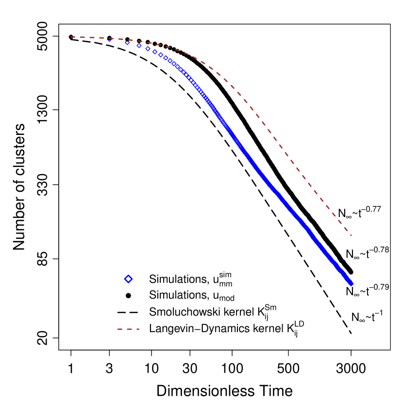
Figure 9: Total number of clusters as a function of time calculated with the simulated intermonomer potential (diamonds), model potential (filled circles), numerical solution of the agglomeration equation with the Smoluchowski kernel (long-dashed line) and with Langevin-Dynamics kernel (short-dashed line).

The results of the simulations (with both potentials) for the total number of clusters and the numerical solution of the agglomeration equation with $K^{Sm}$ and $K^{LD}$ are shown in Fig. 9. The numerical solution of the agglomeration equation with the Langevin-Dynamics kernel (short dashes) shows good agreement with the simulations (dots, simulated intermonomer potential) The early-time agreement is attributed to the Fuchs correction factor, an observation also made in Ref. LorenzoJAS .

The time decay of the total cluster number was fitted to a power law $N_{\infty}\sim t^{-\xi}$ at times $2500\leq t\leq 3000$. For the Langevin-Dynamics kernel we find $\xi=0.77$, a value close to the exponent determined from the numerical simulations ($\xi=0.78$ and $\xi=0.79$ for model and the simulated potentials, respectively) and to $\xi=0.74$ expected for homogeneous kernels. The Smoluchowski kernel exponent is considerably different, $\xi=1$. The slight difference between calculated and theoretical exponents is attributed to the slow approach to the asymptotic limit of the agglomeration equation: the asymptotic limit is reached at times about one order of magnitude longer than the duration of the simulations, primarily due to the Fuchs factor. Finally, we note that, as expected, the Van der Waals attraction enhances the agglomeration rate (compare the simulation results with the two potentials), as noted in Ref. videcoq .

V.5 Collision kernel elements

Collision kernel elements may be obtained by ensemble averaging Eq. (19) over the 10 initial conditions, i.e.,

$$\frac{\langle N_{ij}(t)\rangle}{V\delta t_{\textrm{sam}}}=(2-\delta_{ij})K_{ij}\langle n_{i}(t)n_{j}(t)\rangle\quad.$$ (36)

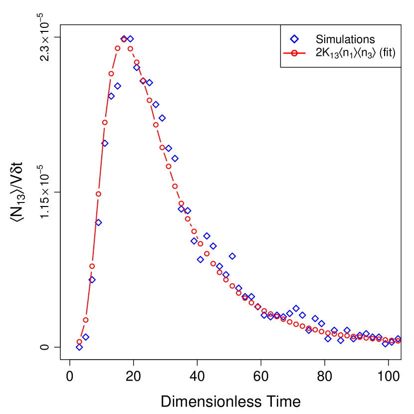
Figure 10: Determination of kernel element $K_{13}$: $\langle N_{13}\rangle/\delta t$ diamonds, $2K_{13}\langle n_{1}\rangle\langle n_{3}\rangle$ with the fitted value of $K_{13}$ circles.

We found that the average of the nonlinear term decouples, $\langle n_{i}n_{j}\rangle=\langle n_{i}\rangle\langle n_{j}\rangle$, to the accuracy of our simulations. We recorded cluster collisions every $\delta t_{\textrm{sam}}$, to avoid counting ternary collisions. We had enough data to calculate only a few kernel elements $K_{ij}$ for low $i$ and $j$ indexes. Figure 10 shows an example of the fitting procedure to determine $K_{13}$ from $\langle N_{13}\rangle/(V\delta t_{\textrm{sam}})$ and $\langle n_{1}\rangle\langle n_{3}\rangle$. The calculated kernel elements $K_{ij}$ are reported in Table 3, and they are compared to the analytical values of $K_{ij}^{LD}$. Kernel elements are scaled to the diagonal of the Smoluchowski kernel $K^{Sm}_{ii}=8\pi D_{1}$. We note an excellent agreement for the $\{(1,1),(1,2),(2,2)\}$ elements. These kernel elements are important in the early-time behaviour of $N_{\infty}(t)$, and therefore they are responsible for the agreement of the numerical simulations with the numerical solution of the agglomeration equation at early times, as shown in Fig. 9.

VI Summary and conclusions

The static structure and diffusive properties of aggregates formed in a quiescent fluid by the collision, and subsequent binding, of spherical monomers were investigated via Langevin dynamics, in the limit of small Knudsen number (continuum regime). The Langevin equations of motion of a collection of diffusing and interacting monomers were solved numerically using a package for generic molecular dynamics simulations with a Langevin thermostat. Two intermonomer interaction potentials were used: a model potential and a potential that arises from the integration of the Lennard-Jones intermolecular potential over the volume of two monomers. Both potentials are spherically symmetric and rapidly decaying. Aggregates were identified during post-processing by considering them to be the connected components of a non-directed graph.

The static structure of the generated aggregates was described in terms of their average fractal dimension and cluster coordination number. We found that the aggregate fractal dimension varied with time from an early-time value characteristic of monomer-cluster agglomeration, ($d_{f}=2.25\pm 0.05$), as determined by local monomer rearrangement and restructuring, to a late-time value characteristic of cluster-cluster agglomeration ($d_{f}=1.56\pm 0.02$), a value dependent on the attractive range of the intermonomer potential. The time dependence of the fractal dimension was linked to the dynamics of two cluster populations, small clusters ($k\leq 15$) at early times and large clusters ($k>15$) at late times. The average cluster fractal dimension, thus, was related to the dominant agglomeration mechanism. The generated aggregates had a cluster coordination number, defined as the mean number of first neighbours of a monomer in a cluster, of more than five (at late times) suggesting that the clusters were compact and not porous. The generated clusters were long, compact, and tubular with a high mean coordination number and low fractal dimension.

We argued that these two salient features of aggregate morphology, small-scale local compactness (evident at the early stages of the agglomeration process) and longer-scale tubular structure (evident at later stages of the agglomeration process), were a consequence of properties of the monomer-monomer interaction potential. The small-scale structure is determined by the isotropy of the potential that allows short-time local reorientation of bonded monomers induced by the thermal noise. Monomers are free to rearrange to maximize their interaction with other monomers, since there is no angular potential to hinder bending of monomer-monomer bonds, under the constraint that monomer-monomer bonds are not stretched. The large-scale structure is determined by the potential interaction range. Colliding, locally compact, clusters rearrange locally at the point of contact: the attractive interaction range of the potential used in the simulations was too short to induce larger-scale rearrangement. Increasing the attractive range would lead to more spherical aggregates. After the initial rearrangements the aggregates remained rigid till the next collision.

The dynamic cluster properties were analyzed in terms of the cluster translational diffusion coefficient. We found that the diffusion coefficient of a $k$-mer scaled with cluster size as $D_{k}\propto k^{-1}$: aggregates diffuse like massive monomers. Furthermore, the average (per-unit-mass) friction coefficient of a monomer in a $k$-monomer cluster was found to equal the (per-unit-mass) friction coefficient of an isolated monomer. Hence, the friction coefficient of a monomer in a cluster was determined to be independent of its state of aggregation, an approximation referred to as free draining approximation: the average monomer shielding factor of the generated clusters was unity. We argued that this diffusive behaviour is a consequence of the absence of shielding in the Langevin equations. This is an inevitable consequence of the usual application of Langevin simulations, unless a (time dependent) shielding coefficient is explicitly introduced in random force term of the Langevin equations. The shielding coefficient would, as a consequence of the Fluctuation Dissipation Theorem, modify the monomer friction coefficient. We, thus, referred to these clusters as ideal clusters, with respect to their transport properties. Similarly, the generated clusters did not have, on average, a preferred orientation.

We also calculated numerically and compared to analytical predictions kernel elements $K_{ij}$ for low indexes. An extensive numerical investigation of the kernel elements is beyond the purpose of the present study, but it can be performed using the methodology described herein.

We conclude that aggregates generated by unshielded Langevin equations of motion of monomers interacting via a central, rapidly decaying potential are on small scales, locally compact, on larger scales tubular, and they diffuse as massive monomers.

Table 1: Overview of cluster static properties.

	Fractal dimension	Prefactor ($R_{g}=ak^{1/d_{f}}$)	Prefactor ($k=k_{g}(2R_{g})^{d_{f}}$)
All clusters	$d_{f}=1.62\pm 0.02$	$a=0.242\pm 0.006$	$k_{g}=3.24$
$k\leq 15$	$d_{f}^{mc}=2.25\pm 0.05$	$a_{mc}=0.386\pm 0.009$	$k_{g}^{mc}=1.75$
$15<k$	$d_{f}^{cc}=1.56\pm 0.02$	$a_{cc}=0.218\pm 0.007$	$k_{g}^{cc}=3.65$

Table 2: Overview of cluster diffusive properties. The percentage in parenthesis (fifth column) is the relative difference of the two mobility radii reported in the fourth and fifth columns.

		$k=4$	$k=10$	$k=50$	$k=98$
$D_{k}$	Simulations, Eq. (22)	$1.30\cdot 10^{-1}$	$4.92\cdot 10^{-2}$	$9.48\cdot 10^{-3}$	$4.84\cdot 10^{-3}$
$R_{g}$	Simulations, Fig. (3)	$7.5\cdot 10^{-1}$	$1.14$	$2.12$	$4.70$
$\beta_{k}$	Simulations, Eq. (24)	$9.6\cdot 10^{-1}$	$1.01$	$1.05$	$1.05$
$R_{m}$	Simulations, Eq. (25)	$1.92$	$5.08$	$26.35$	$51.56$
$R_{m}$	Eq. (26) with $\eta_{k}=1$	$2$ ($4\%$)	$5$ ($1.6\%$)	$25$ ($5.4\%$)	$49$ ($5.2\%$)

Table 3: Comparison of kernel elements (expressed in units of $8\pi D_{1}$).

($i,j$)	$K_{ij}^{LD}\;\rm[Eq.\;(\ref{eq:kernel_complete})]$	$K_{ij}\;\rm[Eq.\;(\ref{eq:kernel_nonlin_aver})]$
(${1,1}$)	$0.213$	$0.214$
(${1,2}$)	$0.294$	$0.298$
(${1,3}$)	$0.309$	$0.397$
(${1,4}$)	$0.309$	$0.449$
(${2,2}$)	$0.317$	$0.317$
(${2,3}$)	$0.303$	$0.349$

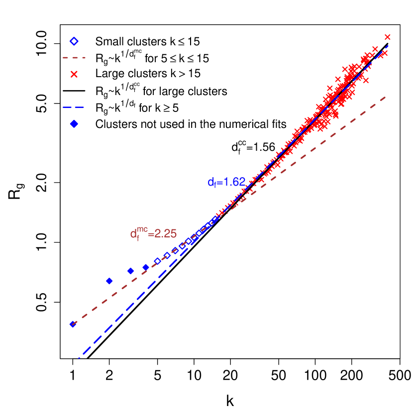
Figure 3: Average radius of gyration as a function of cluster size. Linear fits performed on a double-logarithmic scale for $k>5$ (long-dashed line), $5\leq k\leq 15$ (short-dashed line) and $k>15$ (solid line) (see, also, Table 1).

References

- (1) A.V. Filippov, J. Colloid Interface Sci. 229, 184 (2000).
- Filippov et al. (2000) A.V. Filippov, M. Zurita, and D.E. Rosner, J. Colloid Interface Sci. 229, 261 (2000).
- (3) R.D. Mountain, G.W. Mulholland, and H. Baum, J. Colloid Interface Sci. 114, 67 (1986).
- (4) A. Gutsch, S.E. Pratsinis, and F. Loeffler, J. Aerosol Sci. 26, 187 (1995).
- (5) M.C. Heine and S.E. Pratsinis, Langmuir 23, 9882 (2007)
- (6) L. Maedler, A.A. Lall, and S.K. Friedlander, Nanotechnology 17, 4783 (2006).
- (7) A. Videcoq, M. Han, P. Abélard, C. Pagnoux, F. Rossignol, and R. Ferrando, Physica A 374, 507 (2007).
- (8) M. Hutter, J. Colloid Interface Sci. 231, 337 (2000).
- (9) P. Kulkarmi and P. Biswas, Aerosol Sci. Technol. 38, 541 (2004).
- (10) V. Becker and H. Briesen, Phys. Rev. E 78, 061404 (2008).
- (11) A. Keller, M. Fierz, H.C. Siegmann, and A. Filippov, J. Vac. Sci. Technol. A 19, 1 (2001).
- (12) T.H. Cormen, C.E. Leiserson, R.L. Rivest, and C. Stein, Introduction to algorithms, 2nd edn. (MIT Press, Cambdridge MA, 2001).
- (13) M. Kostoglou and A.G. Konstandopoulos, J. Aerosol Sci. 32, 1399 (2001).
- (14) H. Risken, The Fokker-Planck Equation, 2nd edn., (Springer, Berlin, 1989).
- (15) P. Meakin, Phys. Rev. B 29, 2930 (1984).
- (16) J.C. Fernández-Toledano, A. Moncho-Jordá, F. Martinez-Lopez, A.E. Gonzalez, and R. Hidalgo-Alvarez, Phys. Rev. E 75, 041408 (2007).
- (17) D. Frenkel, B. Smit, Understanding Molecular Simulation, 2nd edn. (Academic Press, San Diego, 2002).
- (18) M. Lazaridis and Y. Drossinos, Aerosol Sci. Technol. 28, 548 (1998).
- (19) G. Narsimhan and E. Ruckenstein, J. Colloid Interface Sci. 104, 344 (1985).
- (20) S. Rothenbacher, A. Messerer, and G. Kasper, Part. Fibre Toxicol. 5, 1 (2008).
- (21) B.E. Poling, J.M. Prausnitz, and J.P. O’Connell, The properties of gases and liquids, 5th edn. (McGraw-Hill, New York, 2000).
- (22) H.J. Limbach, A. Arnold, B.A. Mann, and C. Holm, Comp. Phys. Comm. 174, 704 (2006).
- (23) T. Soddemann, B. Dünweg, and K. Kremer, Phys. Rev. E 68, 046702 (2003).
- (24) A. Arnold, Ph.D. thesis, Johannes Gutenberg-Universität in Mainz, Germany (2004).
- (25) J. Wedekind and D. Reguera, J. Chem. Phys. 127, 154516 (2007).
- (26) G. Csardi and T. Nepusz, InterJournal Complex Systems, 1695 (2006), URL http://igraph.sf.net.
- (27) C.M. Sorensen and G.C. Roberts, J. Colloid Interface Sci. 186, 447 (1997).
- (28) Ü.Ö. Köylü, Y. Xing, and D.E. Rosner, Langmuir 11, 4848 (1995).
- (29) M.K. Wu and S.K. Friedlander, J. Colloid Interface Sci. 159, 246 (1993).
- (30) A.M. Brasil, T.L. Farias, and M.G. Carvalho, Aerosol Sci. Technol. 33, 440 (2000).
- (31) B.M. Smirnov, Phys. Rep. 188, 1 (1990).
- (32) H. Tanaka and T. Araki, Phys. Rev. Lett. 85, 1338 (2000).
- (33) R. Jullien and P. Meakin, J. Colloid Interface Sci. 127, 265 (1989).
- (34) S.F. Friedlander, Smoke, Dust and Haze, 2nd edn. (Oxford University Press, New York, 2000).
- Goldstein (1950) H. Goldstein, Classical mechanics (Addison-Wesley, Cambridge MA, 1950).
- (36) K. Shoemake, in Graphics Gems IV, edited by P. Heckbert (Academic Press, 1994), p. 222.
- (37) J.J. Kuffner, in Proceeding of the IEEE International Conference on Robotics and Automation (2004).
- (38) L. Isella, B. Giechaskiel, and Y. Drossinos, J. Aerosol Sci. 39, 737 (2008).
- (39) M.H. Ernst and P.G.J. van Dongen, Phys. Rev. A 36, 435 (1987).
- (40) P. Ramachandran and G. Varoquaux, in SciPy08: Proceedings of the 7th Python in Science Conference (2008).