Quantum Dynamics of a Microwave Driven Superconducting Phase Qubit Coupled to a Two-Level System

Abstract

We present an analytical and comprehensive description of the quantum dynamics of a microwave resonantly driven superconducting phase qubit coupled to a microscopic two-level system (TLS), covering a wide range of the external microwave field strength. Our model predicts several interesting phenomena in such an ac driven four-level bipartite system including anomalous Rabi oscillations, high-contrast beatings of Rabi oscillations, and extraordinary two-photon transitions. Our experimental results in a coupled qubit-TLS system agree quantitatively very well with the predictions of the theoretical model.

Microscopic two-level systems (TLSs) originating from variety of disorders are ubiquitous in solid state devices. In particular, the TLS plays a double-faced character in the implementation of quantum information processor based on the superconducting qubits RevModPhys.73.357 ; PhysicsToday.58.11 ; Nature.453.1031 . On one side, the TLSs are harmful for the coherent control of qubit states PhysRevLett.93.077003 ; PhysRevLett.95.210503 ; PhysRevB.78.144506 ; PhysRevLett.95.127002 ; PhysRevLett.96.047001 ; PhysRevB.79.094520 ; muller:134517 . Although significant progress has been made to reduce the TLSs in the superconducting qubits QuantumInfProcess.8.81 ; QuantumInfProcess.8.117 it seems however difficult to completely eliminate them in the foreseeable future. On the other side, the TLSs can play a useful role because of their relatively long coherence time PhysRevLett.97.077001 ; NaturePhysics.4.523 ; PhysRevLett.101.157001 ; Nat.Commun. ; PhysRevB.80.094507 . It has been demonstrated that the TLSs in the tunnel barrier of a Josephson junction can function as naturally formed qubits PhysRevLett.97.077001 , quantum memory cells NaturePhysics.4.523 , and quantum beam splitters Nat.Commun. . In either case a thorough understanding of the quantum dynamics of the coupled qubit-TLS system is critical. What’s more, the quantum dynamics of a resonantly driven coupled quantum bipartite system is important not only to fundamental physics Nielsen ; NaturePhysics.4.686 but also to applications such as building scalable quantum information processors based on qubits RevModPhys.73.357 ; PhysicsToday.58.11 ; Nature.453.1031 ; NaturePhysics.6.13 . However, previous theoretical studies mainly focused on a narrow range of the ac driving strengths and only numerical simulations were performed, leaving the physics picture unclear. Consequently, the experimental investigations were incomplete although interesting two-photon Rabi oscillations and anomalous Rabi oscillations have been observed PhysRevLett.93.077003 ; PhysRevB.80.172506 ; PhysRevB.81.100511 . Here, we present an analytical and comprehensive description of the quantum dynamics of a resonantly driven qubit-TLS system that covers a wide range of ac field and qubit-TLS coupling strengths. More importantly, we have experimentally investigated a superconducting phase qubit coupled to the TLSs with all critical system parameters calibrated independently and the data strongly support the results of our theoretical analysis. Therefore, the results reported here, both theoretical and experimental, provide many insights into the dynamics of resonantly driven coupled four-level bipartite quantum systems.

We start by modeling the qubit-TLS system with the Hamiltonian PhysRevLett.101.157001 ; PhysRevB.80.172506 ; PhysRevB.81.100511 ; EPL.71.21 ; PhysRevB.72.024526 ; New.J.Phys.8.103 ; PhysRevB.80.094507 $H(t)=H_{q}(t)+H_{T}+H_{q-T}$. The qubit’s Hamiltonian is $H_{q}(t)=-\frac{\hbar}{2}\omega_{q}\sigma_{z}^{q}+\hbar\Omega_{m}\cos\omega t\sigma_{x}^{q}$, where $\hbar$ is Planck’s constant divided by $2\pi$, $\hbar\omega_{q}$ is the energy level spacing of the qubit, $\Omega_{m}/2\pi$ is the microwave induced Rabi frequency, and $\omega$ is the microwave frequency. The Hamiltonian of the TLS can be written as $H_{T}=-\frac{\hbar}{2}\omega_{T}\sigma_{z}^{T}$, where $\hbar\omega_{T}$ is the energy level spacing of the TLS. The interaction Hamiltonian then is $H_{q-T}=\hbar\Omega_{c}\sigma_{x}^{q}\otimes\sigma_{x}^{T}$, where $\Omega_{c}$ is the coupling strength between the qubit and the TLS, $\sigma_{x,y,z}^{q}$ ($\sigma_{x,y,z}^{T}$) are the Pauli operators acting on the states of the qubit (TLS). Such $\sigma_{x}$ coupling is usually found in NMR and other systems RevModPhys.73.357 ; RevModPhys.76.1037 . To understand the underlying physics more clearly, we choose the interaction picture and make a transformation to a rotating frame, denoting the ground state and excited state of the qubit (TLS) as $|0\rangle$ and $|1\rangle$ ($|g\rangle$ and $|e\rangle$), respectively. In the resonant case, i.e., $\omega=\omega_{q}=\omega_{T}$, the Hamiltonian for the coupled system can be simplified as PhysRevB.80.094507

$$H^{\prime}=\hbar\left(\begin{array}[]{cccc}0&\Omega_{m}/2&0&0\\ \Omega_{m}/2&0&\Omega_{c}&0\\ 0&\Omega_{c}&0&\Omega_{m}/2\\ 0&0&\Omega_{m}/2&0\\ \end{array}\right),$$ (1)

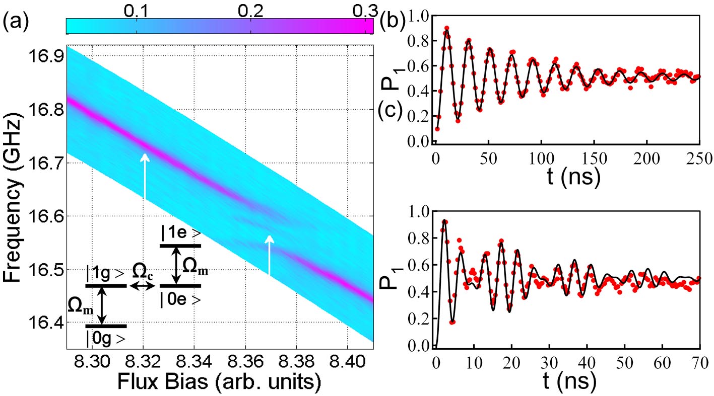
Figure 1: Spectroscopy and coherent oscillations. (a) Spectroscopy of the qubit versus the flux bias with a splitting at $f=16.572$ GHz due to the coupling of the qubit-TLS. (b) Usual Rabi oscillation with the damping time $T_{R}\approx 81.5$ ns at $f=16.728$ GHz (arrow in the left) where the effect of the TLS is negligible. (c) Coherent oscillation at the avoided crossing (arrow in the right) shows quantum beating due to the interference of Rabi oscillations in the coupled system. In (b) and (c), the red dots are the experimental results and the solid lines are the theoretical results.

where the basis states are $|0g\rangle$, $|1g\rangle$, $|0e\rangle$, and $|1e\rangle$ (inset of Fig. 1(a)). It is noticed that the Hamiltonian (1) has the same form as that of the four coupled quantum pendulums Feynman . The simplest way to analyze such system is to find the stationary solutions without considering dissipation, which only affects the amplitude of the probability. The eigenvalues of the Hamiltonian (1) can be easily obtained in the form: $\lambda_{1}=(\Omega_{mc}+\Omega_{c})/2$, $\lambda_{2}=(\Omega_{mc}-\Omega_{c})/2$, $\lambda_{3}=-(\Omega_{mc}-\Omega_{c})/2$, $\lambda_{4}=-(\Omega_{mc}+\Omega_{c})/2$, with $\Omega_{mc}=\sqrt{\Omega_{m}^{2}+\Omega_{c}^{2}}$. The time evolution of the system can be described by $|\Psi(t)\rangle=\sum_{i=1}^{4}c_{i}|\psi_{i}\rangle e^{-i\lambda_{i}t}$, where $|\psi(i)\rangle$ is the eigenfunction of the Hamiltonian (1) corresponding to $\lambda_{i}$. Thus we can obtain the probability of being in state $|\phi\rangle$ ($\phi=0$g, 1g, 0e, 1e):

$$P_{\phi}=\sum_{i,j}c_{j}^{\ast}c_{i}\langle\psi_{j}|\phi\rangle\langle\phi|\psi_{i}\rangle e^{-i(\lambda_{i}-\lambda_{j})t}.$$ (2)

Note that the temporal oscillation of $P_{\phi}$ is composed of $C_{4}^{2}=6$ frequencies. However, only four frequencies are observable because there are two pairs of double degeneracies: $\Omega_{1}=|\lambda_{1}-\lambda_{4}|=\Omega_{mc}+\Omega_{c}$, $\Omega_{2}=|\lambda_{2}-\lambda_{3}|=\Omega_{mc}-\Omega_{c}$, $\Omega_{3}=|\lambda_{1}-\lambda_{3}|=|\lambda_{2}-\lambda_{4}|=\Omega_{mc}$, and $\Omega_{4}=|\lambda_{1}-\lambda_{2}|=|\lambda_{3}-\lambda_{4}|=\Omega_{c}$. Assuming the system is initially prepared in $|\Psi(0)\rangle=|0g\rangle$, it is easy to obtain $P_{\phi}$:

$$\left\{\begin{array}[]{ll}P_{0g}=\frac{4a^{2}b^{2}}{N^{2}}[\frac{a^{4}+b^{4}}{2a^{2}b^{2}}+\frac{a^{2}}{2b^{2}}\cos\Omega_{1}t+\frac{b^{2}}{2a^{2}}\cos\Omega_{2}t+\cos\Omega_{3}t&\\ +\cos\Omega_{4}t]&\\ P_{1g}=\frac{4a^{2}b^{2}}{N^{2}}[1-\frac{1}{2}\cos\Omega_{1}t-\frac{1}{2}\cos\Omega_{2}t-\cos\Omega_{3}t+\cos\Omega_{4}t]&\\ P_{0e}=\frac{4a^{2}b^{2}}{N^{2}}[1+\frac{1}{2}\cos\Omega_{1}t+\frac{1}{2}\cos\Omega_{2}t-\cos\Omega_{3}t-\cos\Omega_{4}t]&\\ P_{1e}=\frac{4a^{2}b^{2}}{N^{2}}[\frac{a^{4}+b^{4}}{2a^{2}b^{2}}-\frac{a^{2}}{2b^{2}}\cos\Omega_{1}t-\frac{b^{2}}{2a^{2}}\cos\Omega_{2}t+\cos\Omega_{3}t&\\ -\cos\Omega_{4}t]&\\ \end{array}\right.,$$ (3)

where $a=\Omega_{m}/2$, $b=(\Omega_{mc}+\Omega_{c})/2$ and $N=\left[\Omega_{m}^{2}+(\Omega_{mc}+\Omega_{c})^{2}\right]/2$ being the normalization factor. Apparently, the populations will oscillate in time with four frequencies. These analytical results form the foundation for a thorough understanding of the coupled qubit-TLS system. Moreover, these general results are also valid for a wide variety of four-level quantum bipartite systems with resonant ac drive. Based on the results many seemingly counterintuitive phenomena in this type of four-level systems become straightforward to understand both qualitatively and quantitatively.

In the experiments involving the TLSs, the quantity one usually measures is the probability of finding the qubit in state $|1\rangle$, i.e., $P_{1}=P_{1g}+P_{1e}$:

$$\begin{array}[]{ll}P_{1}=\frac{4a^{2}b^{2}}{N^{2}}\left[\frac{(a^{2}+b^{2})^{2}}{2a^{2}b^{2}}-\frac{a^{2}+b^{2}}{2b^{2}}\cos\Omega_{1}t-\frac{a^{2}+b^{2}}{2a^{2}}\cos\Omega_{2}t\right].&\end{array}$$ (4)

It is interesting to notice that although there are four frequency components in each $P_{\phi}$ (Fig. 2(a) and Fig. 2(b)), only two of them appear in $P_{1}$ (Fig. 2(d)). Moreover, $\Omega_{m}$ and $\Omega_{c}$ define three regimes for the bipartite system, which show significantly different behaviors: (i) The strong field regime, $\Omega_{m}/\Omega_{c}\gg 1$; (ii) The intermediate field regime PhysRevLett.93.077003 ; PhysRevB.81.100511 , $\Omega_{m}/\Omega_{c}\approx 1$ ; (iii) The weak field regime PhysRevB.80.172506 , $\Omega_{m}/\Omega_{c}\ll 1$. It should be pointed out that previous works focused only on one of the regimes thereby they could not capture the complete picture. Below, based on Eq. (4), we discuss the behaviors of the resonantly driven qubit-TLS system in the three different regimes one by one. The predicted phenomena are demonstrated experimentally by measuring the spectroscopy and the coherent oscillations in a superconducting phase qubit coupled to the TLSs. The detailed experimental setup and procedures have been described elsewhere Nat.Commun. . Shown in Fig. 1 are examples of the spectroscopy and the coherent oscillations. The splitting caused by the qubit-TLS interaction is clearly observed at 16.572 GHz giving the coupling strength $\Omega_{c}/2\pi\approx 26.5$ MHz. Away from the splitting Rabi oscillation induced by the microwave field has the usual damped sinusoidal form (Fig. 1(b)). When the qubit is biased at the splitting, anomalous oscillations are observed, with interesting features determined by the microwave amplitude as described below.

(i) Strong field regime: Rabi beating

In the strong field limit, i.e., $\Omega_{m}/\Omega_{c}\gg 1$, $b\approx a=\Omega_{m}/2$, $P_{1}$ has a simple form:

$$P_{1}=\frac{1}{4}[2-\cos(\Omega_{m}+\Omega_{c})t-\cos(\Omega_{m}-\Omega_{c})t].$$ (5)

It is known in acoustics that beating happens as an interference between two waves of slightly different frequencies. Here the two frequencies in Eq. (5) are close to each other, i.e, $\Omega_{m}+\Omega_{c}\approx\Omega_{m}-\Omega_{c}\approx\Omega_{m}$, which satisfies the condition of beating very well. To be more clear, we further write Eq. (5) as $P_{1}=\frac{1}{2}(1-\cos\Omega_{m}t\cos\Omega_{c}t)$. This is demonstrated experimentally in Fig. 1(c), in which $P_{1}$ appears to oscillate at $\Omega_{m}$ with the amplitude modulated by a much lower frequency $\Omega_{c}$.

To quantitatively characterize the Rabi beating described above, we define $Q_{b}=\Omega_{m}/2\Omega_{c}$ as the frequency contrast of the beating, which is the number of Rabi oscillation periods between the two nodes of the slow varying envelope. Shown in Fig. 2(c) are the measured oscillations of $P_{1}$ at various microwave powers. As the microwave power is increased, $Q_{b}$ increases from about 2 to 7. Therefore the beating becomes increasingly clear. The largest $Q_{b}$ is determined by $\Omega_{m},$ $\Omega_{c},$ and the decoherence time. The exponential decay of the beating envelop is due to the energy relaxation. In the previous experiments PhysRevLett.93.077003 ; PhysRevB.81.100511 ; Nature.421.823 , anomalous Rabi oscillations due to the coupling between two qubits and qubit-TLS were reported. However, since the condition $\Omega_{m}\gg\Omega_{c}$ is not fulfilled, $Q_{b}$ is generally less than 2 and thus no clear pattern of Rabi beating was observed, although several theoretical works PhysRevB.72.024526 ; EPL.71.21 ; New.J.Phys.8.103 ; claudon:184503 have predicted its existence in the superconducting qubits. Nevertheless, one can always apply the Fourier transform (FT) to obtain the two frequency components, as shown in Fig. 2(d). With the help of FT, low-$Q_{b}$ Rabi beatings can be revealed. Therefore, we argue that our experiment is the first to clearly demonstrate Rabi beating in a superconducting phase qubit. Quantum beating is usually found among the three-level atomic systems and has been applied to resolve the detailed internal structure of matter RevModPhys.74.1153 . Rabi beating in the coupled qubit-TLS systems thus can be utilized as a powerful tool in investigating the origin and properties of the TLS.

In Fig. 2(d), we find that the difference between the two Rabi frequencies obtained from FT is exactly $2\Omega_{c}$, which is independent of the microwave power as expected from Eq. (4). In addition, it is interesting to notice that in the strong field limit the population of finding the TLS in the state $|e\rangle$ has a simple form $P_{e}=P_{0e}+P_{1e}=(1-\cos\Omega_{c}t)/2$, which can be viewed as Rabi oscillation between the subspaces $\{|0g\rangle,|1g\rangle\}$ and $\{|0e\rangle,|1e\rangle\}$ PhysRevB.80.094507 . The oscillation frequency ($\Omega_{c}$) between these two subspaces is half of that ($2\Omega_{c}$) between $|1g\rangle$ and $|0e\rangle$ since the probability of finding the system in $|1g\rangle$ ($|0e\rangle$) in each subspace is exactly $1/2$.

(ii) Intermediate field regime: anomalous Rabi oscillation

In this regime, $\Omega_{m}\approx\Omega_{c}$, the two frequencies in $P_{1}$ are well separated. The frequency contrast of the beating $Q_{b}$ is close to unity and no clear pattern of Rabi beating can be observed, as shown in Fig. 2(c). In particular, in the region of weak ac driving interplay between the two frequencies results in anomalous Rabi oscillations which have been observed previously in various superconducting qubits PhysRevLett.93.077003 ; PhysRevB.81.100511 ; Nature.421.823 . We can extract $\Omega_{c}$ and $\Omega_{m}$ by using FT of the anomalous Rabi oscillations. In this regime, the qubit is most strongly affected by the TLSs. Thus, much care has to be taken when performing quantum information processing if the Josephson junction is the intended qubit only. Since $b$ is always greater than $a,$ the weight of the $\Omega_{1}$ component is smaller than that of $\Omega_{2}$ from Eq. (4) (indicated by the color in Fig. 2). With $\Omega_{m}$ further decreasing to the weak field regime, the frequency $\Omega_{1}$ disappears, and $P_{1}$ oscillates with a single frequency $\Omega_{2}$, which will be discussed in detail below.

(iii) Weak field regime: extraordinary two-photon transitions

In this case, $\Omega_{m}\ll\Omega_{c}$, $P_{0e}+P_{1g}=\frac{8a^{2}b^{2}}{N^{2}}(1-\cos\Omega_{3}t)\ll 1,$ the populations in the states $|1g\rangle$ and $|0e\rangle$ are very small. The system mainly evolves in the subspace spanned by $|0g\rangle$ and $|1e\rangle$. This can be seen more clearly by checking the eigen-wavefunction of the Hamiltonian (1) directly. In the weak field limit, $a\ll b$, we have

$$\left(\begin{array}[]{cccc}|\psi_{1}\rangle\\ |\psi_{2}\rangle\\ |\psi_{3}\rangle\\ |\psi_{4}\rangle\\ \end{array}\right)=\frac{1}{\sqrt{2}}\left(\begin{array}[]{cccc}0&1&-1&0\\ 1&0&0&1\\ -1&0&0&1\\ 0&1&1&0\\ \end{array}\right)\left(\begin{array}[]{cccc}|0g\rangle\\ |1g\rangle\\ |0e\rangle\\ |1e\rangle\\ \end{array}\right).$$ (6)

Obviously, starting from the initial state $|0g\rangle$ the system will evolve in the subspace spanned by $|0g\rangle$ and $|1e\rangle$ in the form of $|\Psi(t)\rangle=(|\psi_{2}\rangle e^{-i\lambda_{2}t}-|\psi_{3}\rangle e^{-i\lambda_{3}t})/\sqrt{2}=\left[(e^{-i\lambda_{2}t}+e^{-i\lambda_{3}t})|0g\rangle+(e^{-i\lambda_{2}t}-e^{-i\lambda_{3}t})|1e\rangle\right]/2$ and it is easy to obtain

$$P_{1}\approx P_{1e}=\frac{1}{2}(1-\cos\Omega_{2}t)\approx\frac{1}{2}(1-\cos\frac{\Omega_{m}^{2}}{2\Omega_{c}}t).$$ (7)

The oscillatory behavior is quite normal (i.e., sinusoidal) except the square dependence of the Rabi frequency on the microwave amplitude, which is the signature of two-photon transitions. Therefore, when the microwave field is weak, we expect two-photon Rabi oscillations to occur, as reported in PhysRevB.80.172506 . Furthermore, Eq. (7) predicts that the stronger the qubit-TLS coupling strength is (larger $\Omega_{c}$), the smaller the oscillation frequency becomes (Fig. 2(e)). Notice that both of these results are counterintuitive because one usually would expect that a stronger qubit-TLS coupling would lead to a faster oscillation and that two-photon transitions would be significant in strong ac fields. These intriguing phenomena can be understood with the help of the energy level structure shown in the lower inset of Fig. 3. When a microwave with $2\omega_{q}$ matching the energy difference between $\left|0g\right\rangle$ and $\left|1e\right\rangle$ is applied, population can be transferred from $\left|0g\right\rangle$ to $\left|1e\right\rangle$ with the help of the intermediate states $\frac{1}{\sqrt{2}}$($\left|1g\right\rangle\pm\left|0e\right\rangle$), although there is no direct coupling between $\left|0g\right\rangle$ and $\left|1e\right\rangle$. However, both of the two intermediate states are off-resonant with the microwave field. Thus the larger $\Omega_{c}$, the greater the detuning, and the smaller the frequency of the two-photon Rabi oscillations PhysRevA.54.4854 . Since the decoherence time of our qubit is relatively short, we use the spectroscopy data to demonstrate our prediction. The spectroscopy data in Fig. 3 were obtained using long microwave pulses. The stationary population generated by the microwave induced transitions is measured. Notice that in the range of frequencies measured two splittings resulting from qubit-TLS coupling can be clearly observed Nat.Commun. , with $2\Omega_{c}/2\pi$ about 20 MHz at 16.590 GHz and 64 MHz at 16.510 GHz, respectively. Inside each splitting there is a stripe in the avoided crossing. These stripes are resonant peaks generated by the two-photon transitions because the positions of the peaks (in frequency) match exactly to one half of the energy difference between $\left|0g\right\rangle$ and $\left|1e\right\rangle$ in the entire flux bias range. The stripe inside the 20 MHz splitting has a higher intensity than that inside the 64 MHz splitting, which agrees with our prediction as discussed above. We calculated the stationary population of the driven qubit-TLS system using the Markovian master equation. Shown in the upper inset of Fig. 3 is the dependence of the spectrum intensity on $\Omega_{c}$. The peak induced by the two-photon transitions (the middle one) disappears as $\Omega_{c}$ increases. On the other hand, the two-photon transition gradually vanishes while the single-photon transition becomes dominant as the microwave power increases. Further increasing microwave power leads to the anomalous Rabi oscillations and Rabi beating.

In summary, we present a theoretical model to describe the quantum dynamics of a resonantly driven superconducting qubit coupled to a TLS. The analytical result gives a clear physical picture of the system’s dynamical behavior and predicts that in a four-level bipartite quantum system depending on the relative strength of the resonant ac driving and the interparticle coupling, high-contrast Rabi beating, anomalous Rabi oscillations, and extraordinary two-photon transitions can occur. All of these phenomena have been unambiguously observed in our experiment using a superconducting phase qubit coupled to the TLSs and the data agree remarkably well with the quantitative prediction of the model. We emphasize that our model not only provides a unified theoretical description of and physical insights into various experimental observations in the superconducting qubits reported in the literature, but can also be applied to understand the dynamics of many other resonantly driven four-level quantum bipartite systems. The model thus forms a solid theoretical foundation and provides clear physical intuition to the design and analysis of coupled bipartite qubit systems for the quantum information processing.

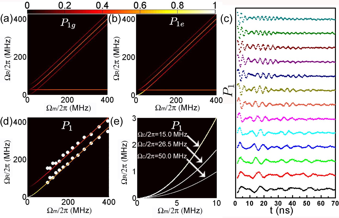
Figure 2: Frequencies $\Omega_{R}$ in $P_{\phi}$. (a) and (b), Four frequencies with different weight (indicated by the color) in $P_{1g}$ and $P_{1e}$ versus $\Omega_{m}$, respectively. (c) Rabi oscillations with the microwave power, at the top of the fridge, increasing from -13 dBm to -1 dBm with a step of 1 dBm from bottom to top. Curves are shifted vertically for clarity. Quantum beating becomes more clear as the amplitude of microwave increases. (d) Frequencies (dots), obtained by the Fourier transformations of the corresponding Rabi oscillations in (c), versus the microwave amplitude. The color lines are the two frequencies in $P_{1}$ obtained from the theoretical analysis. (e) Frequencies in $P_{1}$ induced by the two-photon transitions versus $\Omega_{m}$ with three different $\Omega_{c}/2\pi$: 15.0 MHz, 26.5 MHz, and 50.0 MHz.

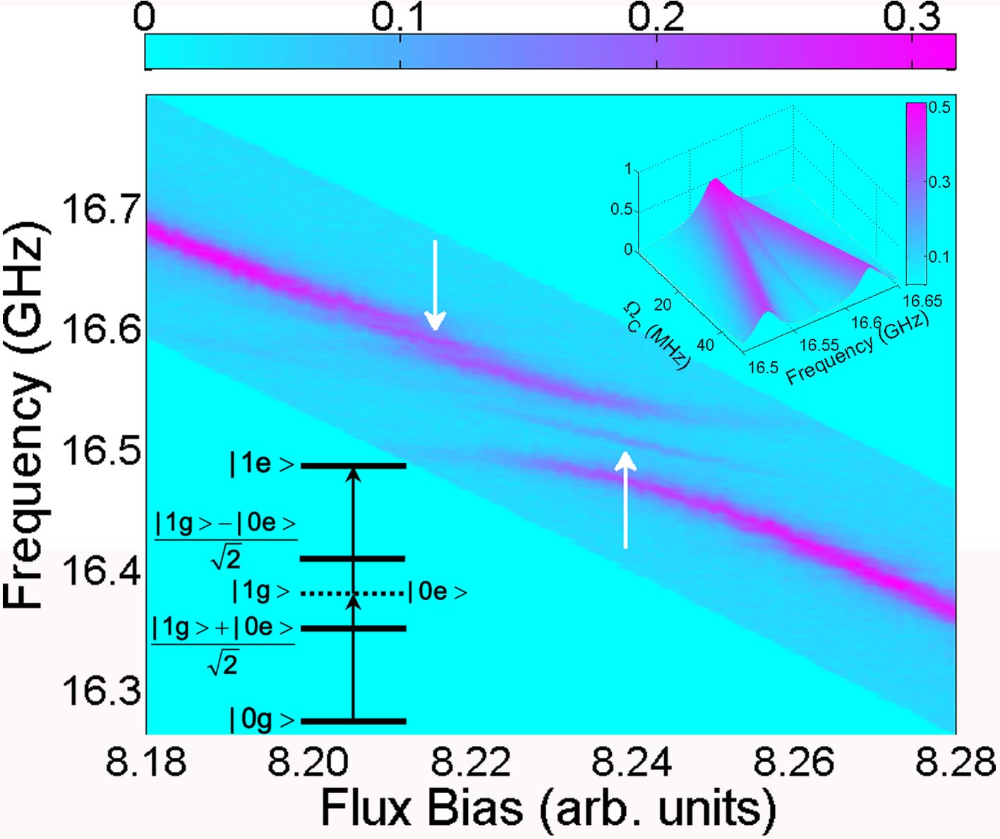
Figure 3: Two-photon transitions. Large $\Omega_{c}$ hinders two-photon transitions, leading to a lower resonant peak in the measured spectrum as marked with arrows. The lower inset shows the energy levels in the qubit-TLS coupled system. The upper inset shows the spectrum density versus $\Omega_{c}$. The outside peaks are due to the stationary population from $\left|0g\right\rangle$ to $\frac{1}{\sqrt{2}}$($\left|1g\right\rangle\pm\left|0e\right\rangle$). The middle peak is due to the two-photon transitions from $\left|0g\right\rangle$ to $\left|1e\right\rangle$.

- (1) Y. Makhlin, G. Schön, and A. Shnirman, Rev. Mod. Phys. 73, 357 (2001).
- (2) J. You and F. Nori, Physics Today 58, 42 (2005).
- (3) J. Clarke and F. K. Wilhelm, Nature 453, 1031 (2008).
- (4) R. W. Simmonds, K. M. Lang, D. A. Hite, S. Nam, D. P. Pappas, and J. M. Martinis, Phys. Rev. Lett. 93, 077003 (2004).
- (5) J. M. Martinis, K. B. Cooper, R. McDermott, M. Steffen, M. Ansmann, K. D. Osborn, K. Cicak, S. Oh, D. P. Pappas, R. W. Simmonds, and C. C. Yu, Phys. Rev. Lett. 95, 210503 (2005).
- (6) Z. Kim, V. Zaretskey, Y. Yoon, J. F. Schneiderman, M. D. Shaw, P. M. Echternach, F. C. Wellstood, and B. S. Palmer, Phys. Rev. B 78, 144506 (2008).
- (7) I. Martin, L. Bulaevskii, and A. Shnirman, Phys. Rev. Lett. 95, 127002 (2005).
- (8) L. Faoro and L. B. Ioffe, Phys. Rev. Lett. 96, 047001 (2006).
- (9) M. Constantin, C. C. Yu, and J. M. Martinis, Phys. Rev. B 79, 094520 (2009).
- (10) C. Müller, A. Shnirman, and Y. Makhlin, Phys. Rev. B 80, 134517 (2009).
- (11) J. M. Martinis, Quantum Inf. Process. 8, 81 (2009).
- (12) R. W. Simmonds, M. S. Allman, F. Altomare, K. D. O. K. Cicak, J. A. Park, M. Sillanp, A. Sirois, J. A. Strong, and J. D. Whittaker, Quantum Inf. Process. 8, 117 (2009).
- (13) A. M. Zagoskin, S. Ashhab, J. R. Johansson, and F. Nori, Phys. Rev. Lett. 97, 077001 (2006).
- (14) M. Neeley, M. Ansmann, R. C. Bialczak, M. Hofheinz, E. L. N. Katz, A. OConnell, H. Wang, A. N. Cleland, and J. M. Martinis, Nature Physics 4, 523 (2008).
- (15) Y. Yu, S.-L. Zhu, G. Sun, X. Wen, N. Dong, J. Chen, P. Wu, and S. Han, Phys. Rev. Lett. 101, 157001 (2008).
- (16) G. Sun, X. Wen, B. Mao, J. Chen, Y. Yu, P. Wu, and S. Han, Nature Communications 1:51 (2010).
- (17) X. Wen, S.-L. Zhu, and Y. Yu, Phys. Rev. B 80, 094507 (2009).
- (18) M. A. Nielsen and I. L. Chuang, Quantum Computation and Quantum Information (Cambridge University Press, Cambridge, 2000).
- (19) F. Deppe, M. Mariantoni, E. P. Menzel, A. Marx, S. Saito, K. Kakuyanagi, H. Tanaka, T. Meno, K. Semba, H. Takayanagi, E. Solano and R. Gross, Nature Physics 4, 686 (2008).
- (20) D. Hanneke, J. P. Home, J. D. Jost, J. M. Amini, D. Leibfried, and D. J. Wineland, Nature Physics 6, 13 (2010).
- (21) A. Lupaşcu, P. Bertet, E. F. C. Driessen, C. J. P. M. Harmans, and J. E. Mooij, Phys. Rev. B 80, 172506 (2009).
- (22) J. Lisenfeld, C. Müller, J. H. Cole, P. Bushev, A. Lukashenko, A. Shnirman, and A. V. Ustinov, Phys. Rev. B 81, 100511 (2010).
- (23) Y. M. Galperin, D. V. Shantsev, J. Bergli, and B. L. Altshuler, Europhys. Lett. 71, 21 (2005).
- (24) L.-C. Ku and C. C. Yu, Phys. Rev. B 72, 024526 (2005).
- (25) S. Ashhab, J. R. Johansson, and F. Nori, New J. Phys. 8, 103 (2006).
- (26) L. M. K. Vandersypen and I. L. Chuang, Rev. Mod. Phys. 76, 1037 (2005).
- (27) R. P. Feynman, The Feynman Lectures on Physics III (Addison-Wesley, 1989).
- (28) Y. A. Pashkin, T. Yamamoto, O. Astafiev, Y. Nakamura, D. V. Averin, and J. S. Tsais, Nature 421, 823 (2003).
- (29) J. Claudon, A. Zazunov, F. W. J. Hekking, and O. Buisson, Phys. Rev. B 78, 184503 (2008).
- (30) D. Budker, W. Gawlik, D. F. Kimball, S. M. Rochester, V. V. Yashchuk, and A. Weis, Rev. Mod. Phys. 74, 1153 (2002).
- (31) A. F. Linskens, I. Holleman, N. Dam, and J. Reuss, Phys. Rev. A 54, 4854 (1996).