Prediction of extreme events in the OFC model on a small world network

Abstract

We investigate the predictability of extreme events in a dissipative Olami-Feder-Christensen model on a small world topology. Due to the mechanism of self-organized criticality, it is impossible to predict the magnitude of the next event knowing previous ones, if the system has an infinite size. However, by exploiting the finite size effects, we show that probabilistic predictions of the occurrence of extreme events in the next time step are possible in a finite system. In particular, the finiteness of the system unavoidably leads to repulsive temporal correlations of extreme events. The predictability of those is higher for larger magnitudes and for larger complex network sizes. Finally, we show that our prediction analysis is also robust by remarkably reducing the accessible number of events used to construct the optimal predictor.

Introduction.–

Self-organized criticality (SOC) is a mechanism by which a large class of spatially extended dynamical systems, starting in a non-equilibrium uncorrelated state, can spontaneously organize into a dynamical critical state with a high degree of correlations jen_book . In particular, a partial synchronization of the elements of the system is usually responsible for building up long range spatial correlations and thereby creating a critical state, in the thermodynamic limit. The emergence of this SOC complex behaviour in physical systems is manifested, for instance, by temporal and spatial scale invariance, i.e. power law or scale free behaviour. SOC has been proposed as a way to model the widespread occurrence of power laws in nature, i.e. the abundance of long-range correlations in space and time – similar to those observed in critical phase transitions stanley – of completely different events, e.g. luminosity of quasars, chemical reactions, evolution, sand-pile models, earthquakes, avalanches, forest burns, heart attacks, market crushes, etc. BTW ; bak_book ; jen_book . Actually, the realistic applicability of SOC models to describe some of these real events is still debated – see, for instance, Refs. yang ; mega ; BTW ; bak_book ; jen_book ; com-corral ; Olami ; lise ; sornette . An important consequence of the presence of SOC scenario is that in the critical state the evolution of the system is completely unpredictable. Indeed, once a SOC system reaches the critical state, arbitrarily large events can be generated intrinsically by the dynamics itself. Another important feature of the SOC behaviour is that no fine-tuning of some external control parameters is required. For a generic initial condition, after some time interval to let the system ‘synchronize’, it drives itself into a critical state. However, in the real world the real systems have a finite size and this unavoidably induces the presence of some extra correlations between following events. Such correlations will be used in the following as a useful source of information on the system evolution and they will allow us to forecast particular events. Actually, we will show that there exists some nontrivial predictability for large but finite system sizes and for the so-called extreme events. The latter can be defined as large deviations from the ‘average’ behaviour of a complex system and are normally caused by the presence of intrinsic dynamical fluctuations. These phenomena and their statistical properties have been intensively studied in literature Schellnhuber ; Albeverio but, however, the mechanisms and dynamics underlying these huge deviations are not always fully clarified. Moreover, the extreme events play an important role in nature and in our daily life because they are often associated to destructive events, e.g. hurricanes, strong earthquakes, etc. In this respect, the predictability of extreme events is urgently desired but also intensely debated debates . In this paper, following the prediction analysis in sand-pile model in Ref. kantz , we will investigate the predictability of such extreme events, by exploiting the time correlations induced by the finiteness of the system, in a SOC model on a complex network recently studied in Refs. Filippo_creta ; carusopre . In other words, on the basis of past observed events, it is possible to predict when the next extreme event will happen and the success probability will increase for ‘more’ extreme events and for larger systems. The latter seems to be in contradiction to our claim that predictability relies on finite size effects, but it is true if the magnitude of avalanches is measured relative to the size of the largest possible avalanche, so that, when comparing predictability in systems of different size, we also compare events of different absolute size.

Model.–

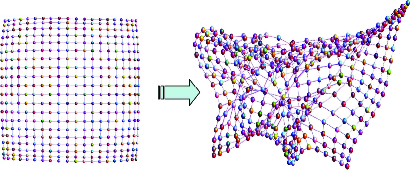
Figure 1: Construction of a small world topology introducing a small fraction ($\sim 2\%$ of the total number of links) of long-range links in a $20$x$20$ square lattice. It corresponds to a rewiring probability equal to $p_{rew}=0.02$.

Here, we analyze one of the most interesting SOC models, i.e. the Olami-Feder-Christensen (OFC) model Olami . Let us consider a two-dimensional ($L$ x $L$) square lattice of $N=L^{2}$ sites, in which each of them carries a real variable $F_{i}$ (initially a random value in $[0,F_{th}]$), representing for instance a seismogenic force, and is connected by a link to its $4$ nearest neighbours. Then, all these variables $F_{i}$ are uniformly and simultaneously increased in order to describe a loading or stress accumulation (e.g., uniform tectonic loading). At some point, when one site becomes unstable, i.e. $F_{i}\geq F_{th}$ with $F_{th}$ being some threshold value, the driving is stopped (no extra time step) and a domino effect happens (discharging or stress release), i.e. an earthquake or avalanche starts. In other terms, one has:

$$F_{i}\geq F_{th}\Rightarrow\left\{\begin{array}[]{l}F_{i}\rightarrow 0\\ F_{nn}\rightarrow F_{nn}+\alpha F_{i}\end{array}\right.$$ (1)

with $nn$ being the set of nearest-neighbor sites of $i$. The magnitude of the domino event will be so defined by the number of these topplings at time step $i$, i.e. $s_{i}$, while $\alpha$ describes the presence of dissipation in the model. In the case of a square lattice, the dynamics is conservative for $\alpha=0.25$, while it is dissipative for $\alpha<0.25$. Here, we will consider a more realistic version of this model, studied recently in Ref. carusopre ; Filippo_creta , in which a small fraction of long-range links was introduced to obtain a small world topology watts . In particular, the presence of a few long-range edges is enough to synchronize the system and both finite-size scaling and universal exponents appear Filippo_creta . The use of a small-world topology is justified also by the fact that long-range spatial correlations have been observed in nature, for instance in earthquake triggering and interaction, where the static stress may involve relaxation processes in the asthenosphere with relevant spatial and temporal long-range effects marsan ; casarot ; cresce ; parsons ; kagan ; turcotte ; palatella ; abe ; corral1 ; tosi ; varotsos . The construction of the small world network from a square lattice of size $L$ is explained in more details in Refs. carusopre ; Filippo_creta . An example of the small world topology construction is qualitatively shown in Fig. (1). Basically, the links of the lattice are rewired at random with a probability $p_{rew}$ and small world transition and self-organized criticality (with finite size scaling with universal critical exponents for the avalanche size probability distribution) are observed at $p_{rew}=0.02$, in the dissipative regime, i.e. $\alpha=0.21$ note . Notice that, in the thermodynamical limit, the size probability distribution is a power-law (without cutoff) and any avalanche size is possible, so both the largest and the mean avalanche size are infinite. However, in a finite size system, i.e. for a finite $L$, this probability distribution is a power law with a cutoff, induced by the finite extension of the lattice, and we will indicate with $s_{max}$ the largest avalanche size. This quantity will be numerically determined in the following. For a generic initial condition, the OFC model on the small world topology, after a transient (discarded later) to build up spatial long-range correlations, reaches a critical state and generate a time series of avalanche size $\{s_{i}\}$, $i=1,\ldots,n$. In particular, we will analyze a time series of $n=10^{8}$ events. Moreover, we define the recurrence time of avalanches of size larger or equal than $\bar{s}$ as the time interval ($j-i$) in between two consecutive events $s_{i}$ and $s_{j}$ such that $s_{i}\geq\bar{s}$ and $s_{j}\geq\bar{s}$, with $j>i$. For infinite lattice size (thermodynamical limit), the recurrence time distribution is an exponential for any $\bar{s}$ since successive events are always uncorrelated to each other. However, as pointed out above, any real system and any numerical simulation involves a finite size and this thermodynamical limit behaviour does hold only for small avalanches ($\bar{s}\ll L^{2}$), which occur in the bulk of the lattice and are not affected by the presence of boundaries. Indeed, the recurrence time distribution of large avalanches will be not exponential but actually one observes the suppression of short time intervals. The reason of this behaviour is the following. After a very large avalanche, the system may relax into a sub-critical state and several time steps are necessary to drive it again into a critical regime. This effect in turns implies some sort of repulsion between ‘extreme’ avalanches. These repulsive correlations are quite weak but useful enough to make predictions on the future occurrence of extreme events.

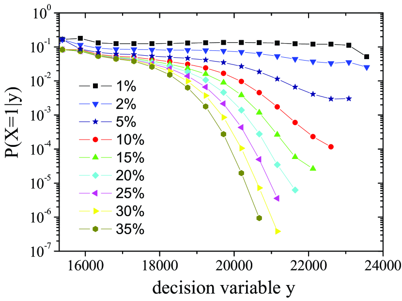
Figure 2: Conditional probability $P(X=1)|y)$ as a function of the decision variable $y$, for events with size exceeding $1\%$, $2\%$, $5\%$, $10\%$, $15\%$, $20\%$, $25\%$, $30\%$, and $35\%$ of the maximal avalanche size $s_{max}$, in the case of $L=128$.

Prediction algorithm.–

Following Ref. kantz , we introduce a Boolean series associated to the events with a size larger than some threshold $\eta$, i.e. $\{X_{i}\}$ with $i=1,\ldots,n$ such that $X_{i}=1$ if $s_{i}>\eta$ and $X_{i}=0$ otherwise. The idea is that, by using information from the past, e.g. from one half of the time series ($i=1,\dots,n/2$), we want to predict if the next event variable $X_{j}$ (with $j=n/2+1,\dots,n$) is $1$ or $0$, i.e. whether the next event will exceed the size $\eta$. In order to do that, we define a decision variable series $\{y_{i}\}$ as follows

$$y_{i}=\sum_{k=1}^{i}a^{k}s_{i-k},\quad 0<a<1,$$ (2)

with $a$ being a time scale tuning the quality of the prediction. Here, for any threshold $\eta$, as in Ref. kantz , $a$ will be chosen of the form $a=\exp\{-1/T(L)\}$ with $T(L=16)=56$, $T(L=32)=112$, $T(L=64)=225$, and $T(L=128)=500$, which are numerically optimized. Notice that in the case, for instance, of $L=128$, $a$ is such that the $1000th$ event before the time $i$, i.e. $k=1000$ in Eq. (2), has a weight $1\%$ smaller than the one used for much smaller $k$. In other words, the time scale of the repulsive correlations, discussed above, can be at most considered of the order of thousands events. Besides, let us stress that $y_{i}$ does depend only on the past events and so from the knowledge of the past time series one wants to forecast the future events. As discussed in Ref. kantz , the possibility of making predictions is subordinated to the fact that the conditional probability $P(X=1|y)$, i.e. the probability for an avalanche with size larger than $\eta$ to occur given a specific value of the decision variable $y$, must show at least a maximum as a function of $y$. This necessary condition for predictability is investigated in our case for several values of $\eta$ in terms of $s_{max}$, as shown in Fig. (2). We find that for small sizes, i.e. $\eta$ equal to a few $\%$ of $s_{max}$, the conditional probability $P(X=1|y)$ has almost a flat behaviour, implying that the probability for an event to happen is completely independent on the past, i.e. no predictability is possible. In this case, the finite-size effects are irrelevant and the behaviour of small avalanches well approximates the temporal features of the thermodynamical limit. However, for large avalanche sizes $P(X=1|y)$ shows a maximum at small values of $y$, i.e. it is more likely to have a large event when only small avalanches happened in the recent past. It is another way to show that extreme events repel each other and between two consecutive ones the system is in a sub-critical state and generates mainly small avalanches. Let us point out also that the maximum of $P(X=1|y)$ is more pronounced for larger $\eta$, i.e. larger events are more predictable. Now, we will describe in a more quantitative way how to make predictions once one knows the decision variable $y$. In particular, one needs to define a probabilistic predictor on $\{y_{i}\}$, defined as a map $y_{i}\mapsto\hat{p}_{i}$, with $\hat{p}_{i}\in[0,1]$. It can be proved that the optimal predictor is simply characterized by the conditional probability, i.e. $\hat{p}_{i}=P(X=1|y_{i})$ Neyman ; Hallerberg ; kantz . In general, this predictor is probabilistic, since it is defined by $P(X=1|y_{i})$, but it can converted into a deterministic one by simply introducing a threshold, as follows

$$X^{pred}_{i} = \left\{\begin{array}[]{ll}1\quad:&\mbox{if}\quad P(X=1|y_{i})>r_{alarm},\\ 0\quad:&\mbox{otherwise,}\end{array}\right.$$ (5)

with $r_{alarm}$ being a control parameter determining the total alarm rate, while $X^{pred}_{i}$ is the predicted value of the Boolean variable $X_{i}$. By increasing the value of $r_{alarm}$, the total alarm rate decreases, i.e. one predicts one event only when the occurrence probability is really high. Of course, a posteriori we may check whether our prediction is right or false by just comparing the variables $X_{i}$ and $X^{pred}_{i}$. On one hand, when $X_{i}=X^{pred}_{i}=1$, the prediction is correct and this event is counted in the so-called hit rate. On the other hand, when $X_{i}\neq X^{pred}_{i}=1$, the prediction is wrong and it does correspond to a false alarm. Notice also that, if $r_{alarm}=0$, the condition in (5) is always satisfied and both rates tend asymptotically to $1$. Instead, for $r_{alarm}$ close to the maximum of $P(X=1|y_{i})$, that inequality does never hold and both rates are zero, i.e. one does not make any prediction.

Specifically, we will use the first half of our avalanche time series of $10^{8}$ events as a training set to construct the predictor, which means that we estimate $P(X=1|y_{i})$ on these data. We then feed this $P(X=1|y_{i})$ with $y_{i}$ values from the second half and compare the outcome to the corresponding boolean values $X_{i}$.

Prediction quality and results.–

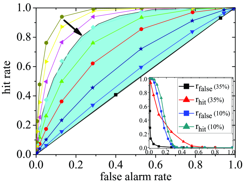
Figure 3: ROC plots for the prediction of extreme events, for events with size exceeding $1\%$, $2\%$, $5\%$, $10\%$, $15\%$, $20\%$, $25\%$, $30\%$, and $35\%$ of the maximal avalanche size $s_{max}$ (from bottom to top), in the case of $L=128$. These curves are squeezed to the colored (blue) area in the case of $L=64$, i.e. the predictability is better for larger system sizes. This behaviour does hold also for other smaller lattice sizes, that we have considered, e.g. $L=16$ and $L=32$. Inset: Hit rate and false alarm rate versus the threshold $r_{alarm}$ (normalized to $\max[P(X=1|y)]$), for $\eta=10\%,35\%\ s_{max}$.

Here, we analyze in more detail the quality of the $y$-based predictions in the case of the OFC model on a small world network, described above. When we use the prediction algorithm, there are two possible errors ($X_{i}\neq X^{pred}_{i}$) : 1) missing an event, i.e. $X_{i}=1$ and $X^{pred}_{i}=0$, ii) false alarm, i.e. $X_{i}=0$ and $X^{pred}_{i}=1$. A possible method to characterize the prediction quality is the Receiver Operating Characteristics (ROC) Egan , which was recently used in Ref. kantz for a prediction analysis in a sand-pile model. It consists of comparing (in ROC plot) the hit rate $r_{hit}$ and the false alarm rate $r_{false}$, as a function of the threshold $r_{alarm}$. The benchmark is the case $r_{hit}=r_{false}$, i.e. the diagonal in the ROC plot. This is the outcome if predictions $X^{pred}_{i}=1$ are made at random times, independent of the values of $y_{i}$. When $r_{hit}>r_{false}$, the predictor is useful and the distance of the ROC curve from the benchmark diagonal is a good indicator of the quality of the prediction. The ROC curves for the model above in the case of $L=128$ are shown in Fig. (3) for different thresholds $\eta$ in terms of the maximum avalanche size $s_{max}$. Note that, increasing the value of $r_{alarm}$, one can get a very large hit rate with a small false alarm rate (i.e., very good prediction). The extreme points of each ROC curve corresponds to the trivial situations: a) $r_{alarm}=0$, with $r_{hit}=r_{false}=1$, b) $r_{alarm}=\max P(X=1|y_{i})$ with $r_{hit}=r_{false}=0$. Let us stress that the predictability is better for larger threshold avalanche sizes. In the inset of Fig. 3, we show the behaviour of the hit rate and the false alarm rate as a function of $r_{alarm}$ normalized to the maximum value of the conditional probability $P(X=1|y)$. When lowering the threshold $r_{alarm}$, the sensitivity increases, and for large avalanches ($\eta$ = 35%), the hit rate starts to rise much earlier than the false alarm rate, indicating the predictive skill.

We have applied this analysis also to smaller system sizes, e.g. $L=16,\;32,\;64$. There are two essential results: For given system size, we always detect some nontrivial predictability of large events, and the predictability is the better the larger the events we intend to predict. This is an evident consequence of the fact that these are more strongly affected by the finiteness of the network. When comparing different system sizes and predicting events of identical magnitude, the smaller system is better predictable. In this respect, the predictability asymptotically vanishes for infinite system size, as expected. If, however, we measure event magnitudes as percent of $s_{max}$, then larger systems are better predictable. For instance, for $L=64$, all ROC curves are squeezed to the blue area in Fig. (3) and the prediction quality is lower that in the case of $L=128$. Finally, we consider how the predictability quality changes by varying the total number of events in the time series, i.e. $n$. Indeed, a so large number of events, like $10^{8}$, could be not accessible for real phenomena. However, in Fig. 4, we show the optimal prediction quality, measured as the largest distance of the ROC curve from the benchmark ($r_{hit}=r_{false}$), and the corresponding hit rate and false alarm rate as a function of the total number of events $n$. We find that the predictability is similar even constructing the decision variable on a number of events which is three orders of magnitude smaller than the one used above. In other words, this prediction analysis seems to be also quite robust with respect to the size of the accessible sample.

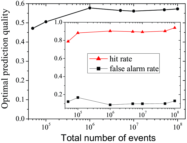
Figure 4: Optimal prediction quality, measured as the largest distance of the ROC curve from the benchmark ($r_{hit}=r_{false}$), versus $n$, in the case of $L=128$ and $\eta=35\%\ s_{max}$. Inset: Optimal hit and false alarm rates versus $n$. The predictability is not affected by remarkably reducing the number of events used to define the decision variable.

Conclusions and Outlook.–

We have investigated the time series of extreme events generated by a dissipative Olami-Feder-Christensen model on a small world network. The small world property is here essential to create vary large events - without small world, the system is not truly critical carusopre . The presence of finite-size effects induces repulsive time correlations between consecutive extreme events and this can be used to make predictions. In particular, we have considered a decision variable which keeps record only of the recently past events and, by using the conditional probability as optimal predictor, we have shown that the predictability quality is really good for large avalanche sizes and for larger networks. In this respect, we have applied a ROC analysis and found that the ratio hit rate/false alarm rate can be remarkably high when considering ‘more extreme’ events. Therefore, these results show that, although the SOC models can be applied to describe very well real events (implying also that they are uncorrelated in time), however, the fact that real physical systems and practical models have a finite size can be exploited to extract information from the extra temporal correlations, induced by the finite-size effects, and forecast the occurrence of extreme events. Interestingly enough, the quality of the predictability is higher for larger systems and for more ‘catastrophic’ events, whose predictability is, of course, even more urgently desired. Finally, although maybe most real phenomena may not share the properties of the SOC model analyzed above, our results suggest to exploit the presence of, though weak, temporal correlations (not necessarily coming from finite-size effects, but also from other sources), to try to forecast extreme events.

- (1) H. Jensen, Self-Organized Criticality (Cambridge Univ. Press, New York, 1998).
- (2) E. Stanley, Introduction to Phase Transitions and Critical Phenomena, (Oxford University Press, 1987).
- (3) P. Bak, How Nature Works: The Science of Self-Organized Criticality (Copernicus, New York, 1996).
- (4) P. Bak et al., Phys. Rev. Lett. 59, 381 (1987); Phys. Rev. A 38, 364 (1988).
- (5) X. Yang et al., Phys. Rev. Lett. 92, 228501 (2004).
- (6) M. S. Mega et al., Phys. Rev. Lett. 92, 129802 (2003).
- (7) A. Helmstetter et al., Phys. Rev. E 70, 046120 (2004).
- (8) A. Corral, Phys. Rev. Lett. 95, 159801 (2005).
- (9) Z. Olami et al., Phys. Rev. Lett. 68, 1244 (1992).
- (10) S. Lise, M. Paczuski, Phys. Rev. Lett. 88, 228301 (2002).
- (11) A. Bunde, J. Kropp, H.J. Schellnhuber (Eds.), The Science of Disasters. Climate Disruptions, Heart Attacks, and Market Crashes (Springer, Berlin, 2002).
- (12) S.A. Albeverio, V. Jentsch, H. Kantz (Eds.), Extreme Events in Nature and Society (Springer, Berlin, 2006).
- (13) Nature debates, Is the reliable prediction of individual earthquakes a realistic scientific goal? (1999), at http://www.nature.com/nature/debates/earthquake/ equake-contents.html
- (14) A. Garber et al., Phys. Rev. E 80, 026124 (2009); A. Garber, H. Kantz, Eur. Phys. J. B 67, 437 (2009).
- (15) F. Caruso et al., Phys. Rev. E, 75, 055101(R) (2007).
- (16) F. Caruso et al., Eur. Phys. Journ. B 50, 243-247 (2006).
- (17) D.J. Watts, S.H. Strogatz, Nature 393, 440 (1998).
- (18) T. Parsons, J. Geophys. Res. 107, 2199 (2002).
- (19) Y.Y. Kagan, D.D. Jackson, Geophys. J. Int. 104, 117 (1991).
- (20) D.L. Turcotte, Fractals and Chaos in Geology and Geophysics (Cambridge Univ. Press, 1997).
- (21) M.S. Mega et al., Phys. Rev. Lett. 90, 188501 (2003).
- (22) S. Abe, N. Suzuki, Europhys. Lett. 65, 581 (2004).
- (23) D. Marsan, C.J. Bean, Geophys. J. Int. 154, 179-195 (2003).
- (24) E. Casarotti et al., Earth and Planetary Science Letters 191, 75-84 (2001).
- (25) L. Crescentini et al., Science 286, 2132 (1999).
- (26) A. Corral, Phys. Rev. Lett. 92, 108501 (2004).
- (27) P. Tosi et al., Annals of Geophysics 47, 1849 (2004).
- (28) P. A. Varotsos et al., Phys. Rev. E 72, 041103 (2005).
- (29) Note that the presence of SOC behaviour in the dissipative OFC model on small world network was verified also for other values of , i.e. , in Ref. carusopre .
- (30) S. Hallerberg, J. Bröcker, H. Kantz, Nonlinear Time Series Analysis in the Geosciences, Lecture Notes in Earth Sciences, Springer (2008).
- (31) J. Neyman, E. S. Pearson, Philosophical Transactions of the Royal Society of London 231, 289 (1933).
- (32) J. P. Egan, Signal detection theory and ROC analysis (Academic Press, New York, 1975).