Dynamical scaling analysis of the optical Hall conductivity in the quantum Hall regime

Abstract

Dynamical scaling analysis is theoretically performed for the ac (optical) Hall conductivity $\sigma_{xy}(\varepsilon_{F},\omega)$ as a function of Fermi energy $\varepsilon_{F}$ and frequency $\omega$ for the two-dimensional electron gas and for graphene. In both systems, results based on exact diagonalization show that $\sigma_{xy}(\varepsilon_{F},\omega)$ displays a well-defined dynamical scaling, for which the dynamical critical exponent as well as the localization exponent are fitted and plugged in. A crossover from the dc-like bahavior to the ac regime is identified. The dynamical scaling analysis has enabled us to quantify the plateau in the ac Hall conductivity previously obtained, and to predict that the plateaux structure in ac is robust enough to be observed in the THz regime.

Introduction —

Dynamics of electrons in the integer quantum Hall effect (QHE) is an interesting, hitherto not fully explored problem. Theoretically, the question is how the static Hall conductivity, which may be regarded as a topological quantityThouless et al. (1982); Hatsugai (1993), evolves into the optical Hall conductivity, especially in the THz regime where the relevant energy scale is the cyclotron energy.Volkov and Mikhailov (1985); Morimoto et al. (2009); Fialkovsky and Vassilevich (2009) Two of the present authors and Hatsugai have recently shown that the plateau structure in $\sigma_{xy}(\omega)$ is retained in the ac ($\sim$ THz) regime in both the ordinary two-dimensional electron gas (2DEG) and in graphene (described as the massless Dirac model), although the plateau height deviates from the quantized values in ac.Morimoto et al. (2009) The numerical result indicates that the plateau structure remains remarkably robust against disorder, which can be attributed to an effect of localization which dominates the physics of electrons around the centers of Landau levels in disordered QHE systems. However, what is physically significant is not a result for a specific sample size, but the scaling behavior, especially when the localization is relevant in disordered systems. For ac responses, we have to look into the dynamical scaling. Scaling analysis of localization-delocalization transition in the 2DEG QHE has been done for both the static longitudinal conductivity $\sigma_{xx}(\varepsilon_{F})$, where $\varepsilon_{F}$ is the Fermi energy, Huckestein (1995) and for dynamical scaling properties of the longitudinal conductivity $\sigma_{xx}(\varepsilon_{F},\omega)$,Gammel and Brenig (1996) but the dynamical scaling for the Hall conductivity $\sigma_{xy}(\varepsilon_{F},\omega)$ has not been properly addressed for both ordinary and graphene QHE.

With this motivation, here we elucidate the dynamical scaling behavior of the ac Hall conductivity around the plateau to plateau transition to gain a deeper understanding of the optical Hall effect and its robust step structures in the ac region. Namely, when we perform a scaling analysis for the plateau to plateau transition width $W$, the quantity depends on $\omega$. Physically, a new length scale, $L_{\omega}\sim\omega^{-\frac{1}{z}}$, emerges at finite frequencies, where $z$ is the dynamical critical exponent. We have performed the dynamical scaling analysis for both 2DEG and graphene QHE. The quantum Hall effect in graphene is unique in that a zero-energy Landau level (LL) exists, which has no counterpart in the QHE in 2DEG Novoselov et al. (2005). Thus the dynamic scaling is of special interest for the $n=0$ LL in graphene.

Experimentally, scaling properties of $\sigma_{xx}(\varepsilon_{F},\omega)$ was investigated from $\omega=0$ Koch et al. (1991) up to the GHz regime Hohls et al. (2002). Recent advances in optical measurements (e.g., Faraday rotation in magnetic fields) in the THz region have made the study of dynamical response functions feasibleIkebe and Shimano (2008); Ikebe et al. (2010). For graphene, optical properties begin to be studied, among which are experimental transmission spectraSadowski et al. (2006), or theoretical examination of the cyclotron emissionMorimoto et al. (2008). Thus, the physics of dynamical scaling in graphene QHE should be interesting in the THz regime.

Here we shall show that: (i) The ac Hall conductivity obeys a well-defined dynamical scaling. (ii) There is a crossover in the scaling behavior from a dc-like regime to an ac regime, in the latter of which $L_{\omega}$ dominates the scaling. In the former $L/\xi$ dominates the scaling (where $\xi$ is the localization length), while in the latter $L_{\omega}/\xi$ does. (iii) The dynamical critical exponent is found to be $z\simeq 2$ in both the 2DEG and graphene QHE systems as far as the potential disorder is concerned. (iv) The analysis enables us to estimate the plateau to plateau transition width $W$ in the ac regime with $L_{\omega}<L$ to assert that the Hall conductivity maintains the plateau structure at frequencies as high as $\omega\sim 0.1\omega_{c}$, which, for a magnetic field of a few Tesla, covers the THz region. This is an experimentally testable statement.

Formalism —

For the ordinary QHE system as typically realized in GaAs/AlGaAs, the kinetic part of the Hamiltonian is $H_{0}=\frac{1}{2m^{*}}({\bf p}+e{\bf A})^{2}$, where $m^{*}$ is the effective mass of the electron, ${\bf p}=(p_{x},p_{y})$ the momentum, and ${\bf A}$ the vector potential. Disorder is introduced by a random potential $V({\bf r})$ composed of Gaussian scattering centers of range $d$ and density $n_{\mathrm{imp}}$ placed on randomly chosen points ${\bf R}_{j}$:

$$V({\bf r})=\sum_{j}u_{j}\exp(-|{\bf r}-{\bf R}_{j}|^{2}/2d^{2})/(2\pi d^{2}).$$ (1)

For $u_{j}$ we assumed a bimodal distribution $u_{j}=\pm u$ with random signs so that the broadened Landau level is symmetric. A measure of disorder, i.e., the Landau level broadeningAndo (1975), is $\Gamma=2u[n_{\rm imp}/2\pi(\ell^{2}+d^{2})]^{1/2}$. Here we take $d=0.7\ell$, where $\ell=\sqrt{\hbar/eB}$ is the magnetic length, but the result does not change significantly for other choices of $d$. Diagonalization of the Hamiltonian is done for the subspace spanned by the five lowest LL’s for $L\times L$ systems with $L/\ell$ varied over $25,30,35,40$. With wave functions and energy eigenvalues $\epsilon_{a}$ at hand, the optical Hall conductivity is evaluated from the Kubo formula,

$$\sigma_{xy}(\varepsilon_{F},\omega) = \frac{i\hbar e^{2}}{L^{2}}\sum_{\epsilon_{a}<\varepsilon_{F}}\sum_{\epsilon_{b}\geq\varepsilon_{F}}\frac{1}{\epsilon_{b}-\epsilon_{a}}$$ (2)

$$\times \left(\frac{j_{x}^{ab}j_{y}^{ba}}{\epsilon_{b}-\epsilon_{a}-\hbar\omega}-\frac{j_{y}^{ab}j_{x}^{ba}}{\epsilon_{b}-\epsilon_{a}+\hbar\omega}\right),$$

where $j_{x}^{ab}$ is the current matrix elementMorimoto et al. (2009).

The conductance is then averaged over a few thousands samples with different disorder potential realizations. The averaged conductivity is hereafter denoted by the same symbol $\sigma_{xy}(\varepsilon_{F},\omega)$. For the scaling analysis the calculation done for varied sample size $L$, energy $\varepsilon_{F}$ and frequency $\omega$.

For graphene QHE, we employ the two-dimensional effective Dirac model,

$$H=v_{F}{\boldsymbol{\sigma}}\cdot{\boldsymbol{\pi}}+V({\bf r}),$$ (3)

where ${\boldsymbol{\sigma}}=(\sigma_{x},\sigma_{y})$ is the Pauli matrices, ${\boldsymbol{\pi}}={\bf p}+e{\bf A}$, and $V({\bf r})$ the random potentialNomura et al. (2008). The selection rule for the current matrix elements in the Dirac model ($|n|\leftrightarrow|n|\pm 1$ with $n$ the Landau index) is distinct from that ($n\leftrightarrow n\pm 1$) for 2DEG.

Raw results for the Optical Hall Conductivity —

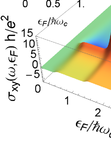
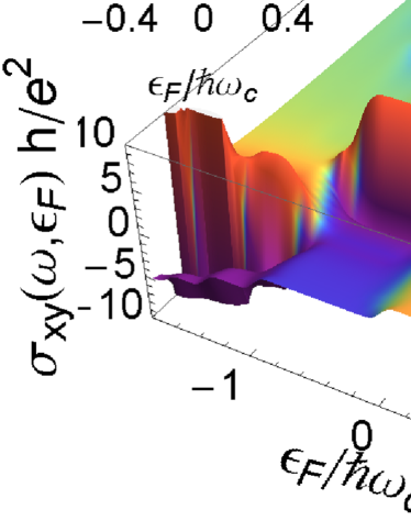
(a)	(b)
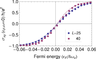
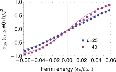
(c)	(d)

Figure 1: $\sigma_{xy}(\varepsilon_{F},\omega)$ plotted against Fermi energy $\varepsilon_{F}$ and frequency $\omega$ for (a) 2DEG, and (b) graphene quantum Hall systems for a pontential disorder with $\Gamma=0.4\hbar\omega_{c}$. Insets are density of states for the lowest ($n=1$) LL (a) and $n=0$ LL (b). (c)The static Hall conductivity $\sigma_{xy}(\varepsilon_{F})$ plotted against $\varepsilon_{F}$ for the graphene QHE system of sizes $L=25,40$. (d) Optical Hall conductivity $\sigma_{xy}(\varepsilon_{F},\omega)$ plotted against $\varepsilon_{F}$ for the graphene QHE system of sizes $L=25,40$ for a fixed $\omega=6\omega_{c}/L^{2}$). The solid lines in (c) and (d) represent fitting with eqn.(5).

The optical Hall conductivity $\sigma_{xy}(\varepsilon_{F},\omega)$ as a function of the Fermi energy $\varepsilon_{F}$ and frequency $\omega$ is displayed for the 2DEG (Fig.1(a)) and graphene (Fig.1(b)) QHE systems. The density of states (DOS) for Landau levels (insets of Fig.1(a,b)) confirms that the Landau level broadening is $\simeq\Gamma$. For each value of $\varepsilon_{F}$, the frequency-dependence is the Hall conductivity can be recognized as the cyclotron resonance. The 2DEG has one resonance at cyclotron frequency $\omega_{c}$ (Fig.1(a)), while the graphene QHE system exhibits a series of resonances, which correspond to the Dirac QHE selection rule $|n|\leftrightarrow|n|\pm 1$ (Fig.1(b)) for the non-uniform set of Landau levels ($\propto\sqrt{n}$). Away from a resonance, a step-like structure is seen in $\sigma_{xy}(\varepsilon_{F},\omega)$ as a function of $\varepsilon_{F}$ even for finite values of $\omega$, although the step heights are no longer quantized. We can attribute this behavior of $\sigma_{xy}(\varepsilon_{F},\omega)$ to the localization property of electrons in QHE systems: As long as $\omega\ll\omega_{c},\Gamma$, the nature of the mobility gap is maintained and $\sigma_{xy}$ remains flat. If we more closely insepct the width $W$ of the plateau to plateau transition, $W$ for a finite $\omega$ in Fig.1(d) is seen to be greater than in the static case in Fig.1(c), although still narrower than $\Gamma$.

We now move on to the sample size dependence of the widths $W(\varepsilon,\omega,L)$ for the static and dynamic Hall conductivities. For the static Hall conductivity $\sigma_{xy}(\varepsilon,0,L)$, we confirm the standard picture, where the plateau to plateau transition width becomes narrower with the sample size $L$ as seen in Fig.1. In the thermodynamic limit, almost all the wave functions are localized, where the localization length diverges like $\xi\sim 1/|\varepsilon_{F}-\varepsilon_{c}|^{\nu}$ toward the center of the LL at $\varepsilon=\varepsilon_{c}$.Aoki and Ando (1985) For finite systems the states whose localization length $\xi$ is larger than the system size $L$ are effectively extended, and contribute to the longitudinal conductivity and the plateau to plateau transition. This suggests the behavior $W\sim L^{-1/\nu}$.

Scaling Analysis — We are now in position to look at the dynamical scaling analysis of the optical Hall conductivity $\sigma_{xy}(\varepsilon_{F},\omega,L)$ and the width $W(\omega,L)$ of the plateau to plateau transition. We expect that the $W$ increasing with $\omega$ and decreasing with $L$ may be captured with some scaling function. For that we have to quantify the width $W$, or the steepness ($\propto 1/W$) of the transition by fitting $\sigma_{xy}(\varepsilon_{F},\omega,L)$ around the transition region for a given LL to some function of $\varepsilon_{F}$ for each value of $\omega$. To describe the transition $\sigma_{xy}/(-e^{2}/h)=0\rightarrow 1$ in the 2DEG QHE we take

$$\sigma_{xy}(\varepsilon_{F},\omega,L)_{\mathrm{2DEG}}=\frac{1}{2}+\frac{1}{2}\tanh\left[\frac{\varepsilon_{F}-\frac{1}{2}\hbar\omega_{c}}{W(\omega,L)}\right],$$ (4)

while for the transition $\sigma_{xy}/(-e^{2}/h)=-1\rightarrow 1$ in graphene QHE we take

$$\sigma_{xy}(\varepsilon_{F},\omega,L)_{\mathrm{graphene}}=\tanh\left(\frac{\varepsilon_{F}}{W(\omega,L)}\right).$$ (5)

The quality of fitting of the plateau to plateau transition by the tanh function is quite satisfactory as can be seen in Fig.1(c,d).

Dynamical scaling analysis for $\sigma_{xy}(\varepsilon_{F},\omega,L)$ is carried out in a similar manner as that for the longitudinal conductivityAvishai and Luck (1996). In this ansatz the optical Hall conductivity is regarded to depend on Fermi energy and frequency only through the ratios $L/\xi$ and $L_{\omega}/\xi$. Here we have the localization length, $\xi\sim 1/|\varepsilon_{F}-\varepsilon_{c}|^{\nu}$ where $\varepsilon_{c}$ is the critical energy which coincides with the center of the LL, and $L_{\omega}\sim 1/\omega^{1/z}$. Then the dynamical scaling ansatz for the optical Hall conductivity reads

$$\sigma_{xy}(\varepsilon_{F},\omega,L)=\frac{e^{2}}{h}F((\varepsilon_{F}-\varepsilon_{c})L^{1/\nu},\omega L^{z}),$$ (6)

where $F$ is a universal scaling function. This implies that the width of the plateau to plateau transition scales as

$$W(\omega,L)=L^{-1/\nu}f(\omega L^{z}),$$ (7)

where $f$ is a universal function deduced from $F$. The first factor on the right-hand side makes the plateau to plateau transition width narrower for larger systems and dictates the dc scaling, while the second factor $f$ describes the dynamical scaling.

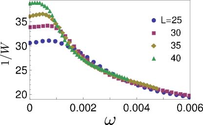
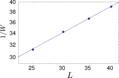
(a)	(b)

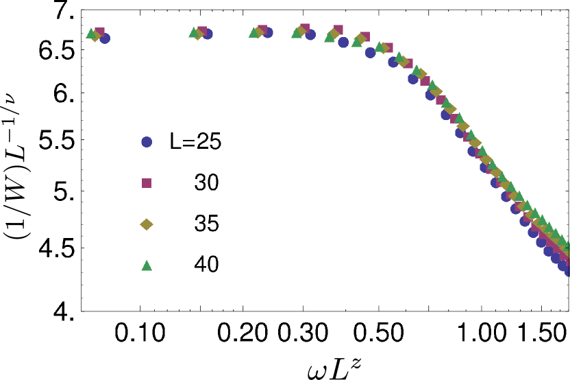
(c)

Figure 2: Dynamical scaling analysis for the 2DEG QHE system with $\Gamma=0.4\hbar\omega_{c}$ and $L=25-40$: (a) The inverse width $1/W$ plotted against the frequency $\omega$, (b) the inverse width $1/W$ plotted against the sample size $L$, from which the localization exponent $\nu=2.1\pm 0.2$ is obtained, and (c) rescaled inverse width $\frac{1}{W}L^{-1/\nu}$ plotted against the rescaled frequency $\omega L^{z}$ with a fitted dynamical critical exponent $z=1.8\pm 0.2$. $W,\omega,L$ are measured, respectively, in units of $\hbar\omega_{c},\omega_{c},\ell$.

In Fig.2 we show the scaling of inverse transition width, $1/W(\omega,L)$, for the 2DEG QHE system. By examining first the inverse width $1/W(\omega=0)$ for the static case against system size $L$ in Fig.2(b), we obtain the localization critical exponent $\nu$ from $\log 1/W(\omega=0)=1/\nu\log L+f(0)$, with the result $\nu=2.1\pm 0.2$. This agrees with the accepted value of the static critical exponent in the integer QHE, albeit slightly smaller.

On the other hand, the frequency dependence of the inverse width for a fixed system size $L$ in (Fig.2(a)) clearly exhibits that there are two regions: In the first region $1/W$ stays nearly constant up to some critical frequency that depends on the system size $L$, while in the other the quanitity begins to decrease monotonically with $\omega$. In the latter region, $1/W$ assumes similar values for all the sample sizes studied here as shown in (Fig.2(a)). We can indeed notice that, in the first region we have $L<L_{\omega}$, while in the second $L>L_{\omega}$. If we inspect eqn.7, and assume a power-law form for the scaling function $f$, we can see that the inverse width in the second region should take a ($L$-independent) form, $1/W(\omega)\propto\omega^{-1/z\nu}$. Calculation of the dynamical exponent $z$ should be done for the critical region (i.e. for the transition width not too large), so that we do this around the crossing region where $1/W$ begins to decrease. This happens, typically, for $\omega<0.002\omega_{c}$. With a least square fitting of $\log 1/W(\omega)={\rm const}-\frac{1}{z\nu}\log\omega$, the dynamical critical exponent for the 2DEG QHE system is obtained as $z=1.8\pm 0.2$ .

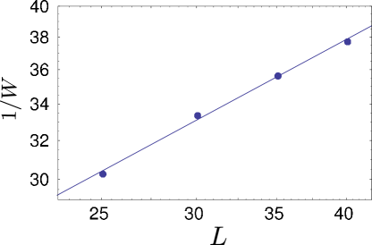
(a)	(b)

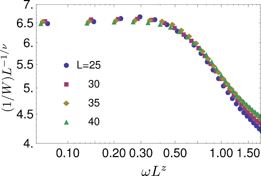
(c)

Figure 3: Dynamical scaling analysis for the graphene QHE system with $\Gamma=0.4\hbar\omega_{c}$ and $L=25-40$: (a) The inverse width $1/W$ plotted against the frequency $\omega$, (b) the inverse width $1/W$ plotted against the sample size $L$, from which the localization exponent $\nu=2.1\pm 0.1$ is obtained, and (c) rescaled inverse width $\frac{1}{W}L^{-1/\nu}$ plotted against the rescaled frequency $\omega L^{z}$ with a fitted dynamical critical exponent $z=1.8\pm 0.2$.

If we now turn to the graphene QHE system, the same analysis is performed based on Fig.3. The frequency dependence of the transition width is rather similar to that for the 2DEG system, as far as the potential disorder assumed here is concerned. The localization exponent $\nu$ and and the dynamical critical exponent $z$ for the graphene system are determined as $\nu=2.1\pm 0.1$ $z=1.8\pm 0.2$, which coincide, within numerical errors, with those for the conventional QHE system. This suggests that the two systems are in the same universality class. As far as the dynamical exponent is concerned, it has been argued by Hikami and Wegner Anderson-Localization-Solid-State-Sciences39 that, when the density of states is an analytic function of energy at a critical point, then $z=d$ ($d$: spatial dimension, which is 2 in the present case). Thus the fact that we get $z\approx 2$ for the 2DEG QHE is commensurate with this conjecture. On the other hand, the density of states for Dirac fermions ($\rho(E)\sim|E|$ for the clean system) is non-analytic, for which one might expect a different behavior in graphene. The absence of deviation in the value of $z$ in Dirac fermions here should come from the fact that the presence of disorder smears the Dirac cone structure in the density of states to make it smooth (Fig.1(b), inset).

Having derived the static and dynamic exponents, we can now actually plot the scaling of the rescaled inverse width against rescaled frequency. This is displayed in Fig.2(c) for 2DEG, and Fig.3(c) (for graphene QHE). It can be judged that the scaling fit is quite good, which indicates that the form of the universal function assumed in eqn(7) is adequate. In the scaling plot we can see more clearly the first region with a constant $\frac{1}{W}L^{-1/\nu}$ for small $\omega L^{z}$, and the second region with a monotonously decreasing $1/W$ for larger $\omega L^{z}$.

Intuitively, we can elaborate as follows: The dynamical response of the QHE system is governed by the magnitude of the localization length relative to two length scales: the system size $L$, and the length $L_{\omega}$ which is the distance over which an electron travels during one cycle, $1/\omega$, of the ac field. Since the localization length diverges as $\xi\sim|\varepsilon-\varepsilon_{c}|^{\nu}$ near the center of LL, and the states contributing to $\sigma_{xy}(\omega)$ should be those that simultaneously satisfy $\xi>L$ and $\xi>L_{\omega}$, the transition width is determined by the smaller length scale $L$ or $L_{\omega}$. In the static limit $\omega=0$, with $L_{\omega}\to\infty$, the system size $L$ determines the transition width $W$Aoki and Ando (1985). When $\omega$ is increased, $L_{\omega}$ decreases. In the low enough frequency region, one still has $L_{\omega}>L$ so that the transition width continues to be determined by the system size. When $L_{\omega}<L$ for higher frequencies, however, $W$ begins to be governed by $L_{\omega}$, and the transition width broadens monotonically with frequency. For even higher frequencies, $L_{\omega}$ becomes so small that the system is far from the critical region, and departure from the scaling should occur.

From the functional form of $f(\omega L^{z})$ in eqn(7), the frequency for which $\omega L^{z}\sim 1$, corresponds to the crossover region where the two regions overlap, that is, $L_{\omega}\sim L$, or $L_{\omega}\sim 1/\omega^{1/z}$. With the dynamical scaling argument with $z\simeq 2$, we end up with $L_{\omega}\sim 1/\omega^{1/2}\sim t^{1/2}$ where $t$ is the diffusion time. Since square-root time evolution is a characteristic of diffusion processes, the dynamical response behavior indicates that the present disordered system is diffusive.

The dynamical scaling here enables us to give an estimate of the transition width $W$ in the THz region (with typically $\omega\sim 0.1\omega_{c}$). In the $L_{\omega}$-dominated regime, one obtains $W\propto\omega^{1/z\nu}$. The proportionality constant can be read out from the numerical result, Fig. 2(c), so that $W/\hbar\omega_{c}\sim 0.2\omega^{1/z\nu}\sim 0.1$ at $\omega=0.1\omega_{c}$. This implies that the plateau structure remains robust up to the THz region, so that experimental measurements should be feasible.

To summarize, dynamical scaling analysis of the optical Hall conductivity in 2DEG and graphene quantum Hall systems have been carried out, while previous studies have focused mainly on the longitudinal conductivity. The dynamical critical exponent $z\simeq 2$ implies that the system is in the diffusive limit. The dynamical critical exponent $z$ is found to be similar between the 2DEG and the graphene QHE system, but we have to re-emphasize that this is as far as the pontential disorder taken here is concernded. It is well-knownKawarabayashi et al. (2009) that the preservation or otherwise of the chiral symmetry in disordered graphene has a profound effect on the $n=0$ graphene Landau level. Thus it is an interesting future problem to look into this effect in terms of the dynamical scaling.

References

- Thouless et al. (1982) D. J. Thouless, M. Kohmoto, M. P. Nightingale, and M. den Nijs, Phys. Rev. Lett. 49, 405 (1982).
- Hatsugai (1993) Y. Hatsugai, Phys. Rev. Lett. 71, 3697 (1993).
- Volkov and Mikhailov (1985) V. Volkov and S. Mikhailov, JETP Letters 41, 476 (1985).
- Morimoto et al. (2009) T. Morimoto, Y. Hatsugai, and H. Aoki, Phys. Rev. Lett. 103, 116803 (2009).
- Fialkovsky and Vassilevich (2009) I. V. Fialkovsky and D. V. Vassilevich, J. Phys. A: Math. Theor. 42, 442001 (2009).
- Huckestein (1995) B. Huckestein, Rev. Mod. Phys. 67, 357 (1995).
- Gammel and Brenig (1996) B. M. Gammel and W. Brenig, Phys. Rev. B 53, R13279 (1996).
- Novoselov et al. (2005) K. Novoselov, A. Geim, S. Morozov, D. Jiang, M. Katsnelson, I. Grigorieva, S. Dubonos, and A. Firsov, Nature 438, 197 (2005).
- Koch et al. (1991) S. Koch, R. Haug, K. Klitzing, and K. Ploog, Phys. Rev. Lett. 67, 883 (1991).
- Hohls et al. (2002) F. Hohls, U. Zeitler, R. Haug, R. Meisels, K. Dybko, and F. Kuchar, Phys. Rev. Lett. 89, 276801 (2002).
- Ikebe and Shimano (2008) Y. Ikebe and R. Shimano, Appl. Phys. Lett. 92, 012111 (2008).
- Ikebe et al. (2010) Y. Ikebe, T. Morimoto, R. Masutomi, T. Okamoto, H. Aoki, and R. Shimano, arXiv:1004.0308 (2010).
- Sadowski et al. (2006) M. L. Sadowski, G. Martinez, M. Potemski, C. Berger, and W. A. de Heer, Phys. Rev. Lett. 97, 266405 (2006).
- Morimoto et al. (2008) T. Morimoto, Y. Hatsugai, and H. Aoki, Phys. Rev. B 78, 073406 (2008).
- Ando (1975) T. Ando, J. Phys. Soc. Jpn. 38, 989 (1975).
- Nomura et al. (2008) K. Nomura, S. Ryu, M. Koshino, C. Mudry, and A. Furusaki, Phys. Rev. Lett. 100, 246806 (2008).
- Aoki and Ando (1985) H. Aoki and T. Ando, Phys. Rev. Lett. 54, 831 (1985).
- Avishai and Luck (1996) Y. Avishai and J. Luck, arXiv:cond-mat/9609265 (1996).
- (19) F. Wegner in Y. Nagaoka and H. Fukuyama, eds., Anderson Localization (Springer, 1982), p.8; S. Hikami, ibid, p.15.
- Kawarabayashi et al. (2009) T. Kawarabayashi, Y. Hatsugai, and H. Aoki, Phys. Rev. Lett. 103, 156804 (2009).