Vectorial structure of a hard-edged-diffracted four-petal Gaussian beam in the far field

Abstract

Based on the vector angular spectrum method and the stationary phase method and the fact that a circular aperture function can be expanded into a finite sum of complex Gaussian functions, the analytical vectorial structure of a four-petal Gaussian beam (FPGB) diffracted by a circular aperture is derived in the far field. The energy flux distributions and the diffraction effect introduced by the aperture are studied and illustrated graphically. Moreover, the influence of the $f$-parameter and the truncation parameter on the non-paraxiality is demonstrated in detail. In addition, the analytical formulas obtained in this paper can degenerate into un-apertured case when the truncation parameter tends to infinity. This work is beneficial to strengthen the understanding of vectorial properties of the FPGB diffracted by a circular aperture.

1 Introduction

In recent years, there have been increasing interests in the study of beam pattern formation. Many beam patterns have potential and practical applications. For example, many researches have been done on dark-hollow beam because it is a powerful tool in precise manipulation and control of microscopic particles [1, 2, 3, 4, 5]. In fact, many other kinds of special laser patterns, such as flower-like patterns and daisy patterns have been observed and investigated [6, 7]. More recently, a new form of laser beam called four-petal Gaussian beam has been introduced and its properties of passing through a paraxial ABCD optical system have been studied [8]. Subsequently, much work has done on four-petal Gaussian beam [9, 10, 11, 12, 13]. As is well known, some researches and applications are conducted in the far field. Meanwhile, in practical applications, however, there are more or less aperture effects, so it is of practical significance to study the influence of a hard-edged aperture on the far-field properties of four-petal Gaussian beam.

In this paper, firstly the power transmissivity of the truncated four-petal Gaussian beam passing through a circular aperture is studied. Secondly, the analytical vectorial structure of four-petal Gaussian beam diffracted by a circular aperture is derived based on vector angular spectrum method [14, 15, 16, 17], stationary phase method [18], and the fact that a circular aperture function can be expanded into a finite sum of complex Gaussian functions [19]. Based on the analytical vectorial structure of four-petal Gaussian beam diffracted by a circular aperture, the energy flux expressions of TE term, TM term and the whole beam are also obtained, respectively. Thirdly, some typical numerical examples are given to illustrate the influence of the diffraction effect introduced by an aperture on the far-field energy flux distributions of four-petal Gaussian beam. Furthermore, the influence of the $f$-parameter and the truncation parameter on the non-paraxiality is demonstrated. Finally, some simple conclusions are given.

2 Analytical vectorial structure of a hard-edged-diffracted four-petal Gaussian beam

Let us consider a half space $z>0$ filled with a linear, homogeneous, isotropic, and nonconducting medium characterized by electric permittivity $\varepsilon$ and magnetic permeability $\mu$. All the sources only lie in the domain $z<0$. For convenience of discussion, we consider a four-petal Gaussian beam with polarization in the x direction, which propagates toward the half space $z\geq 0$ along the z axis. The transverse electric field distribution of the incident four-petal Gaussian beam at $z=0$ plane can be written by [8]

$$E_{x}(x,y,0)=G_{n}\left(\frac{xy}{w_{0}^{2}}\right)^{2n}\exp\left(-\frac{x^{2}+y^{2}}{w_{0}^{2}}\right),n=0,1,2\ldots,$$ (1)

$$E_{y}(x,y,0)=0,$$ (2)

where ${G_{n}}$ is a amplitude constant associated with the order $n$; $w_{0}$ is the $1/e^{2}$ intensity waist radius of the Gaussian term; n is the beam order of the four-petal Gaussian beam. When $n=0$, Eq. (1) reduces to the ordinary fundamental Gaussian beam with the waist being $w_{0}$ at the plane $z=0$. The time factor $\exp(-i\omega t)$ has been omitted in the field expression. After simple calculation, we know that the distance of diagonal petals is given by

$$d=2{(2n)}^{1/2}w_{0}.$$ (3)

According to Eq. 3, the distance $d$ is determined by beam order $n$ and waist size $w_{0}$.

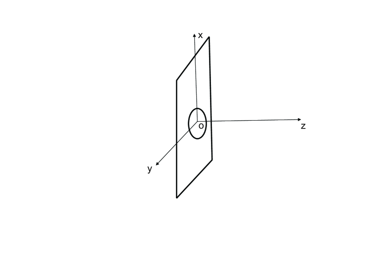
Figure 1: Illustrating the geometry of the screen with a circular aperture and the coordinate system.

Supposing that a hard-edged circular aperture is located at the $z=0$ plane, and the center of the circular aperture is the origin. The geometry for the screen with a circular aperture and the coordinate system is shown in Fig. 1. The corresponding circ function can be written as follows

$$\textmd{circ}(\frac{\rho}{R})=\left\{\begin{array}[]{cc}1,&\rho\leq R,\\ 0,&\rho>R.\\ \end{array}\right.$$ (4)

where $R$ denotes the radius of the circular aperture and $\rho=\sqrt{x^{2}+y^{2}}$ is radial distance. The power transmissivity of the truncated four-petal Gaussian beam is given by

$$T_{n} = \frac{\int^{R}_{0}\int^{2\pi}_{0}\mid E_{x}(\rho,\theta,0)\mid^{2}\rho d\rho d\theta}{\int^{\infty}_{0}\int^{2\pi}_{0}\mid E_{x}(\rho,\theta,0)\mid^{2}\rho d\rho d\theta}$$ (5)

$$= 1-\frac{\Gamma(4n+1,2\beta^{2})}{4n\Gamma(4n)},$$

where $\Gamma(z)=\int^{\infty}_{0}t^{z-1}e^{-t}dt$ is Euler gamma function, and $\Gamma(a,z)=\int^{\infty}_{z}t^{a-1}e^{-t}dt$ is incomplete gamma function. $\beta=R/w_{0}$ is defined as the truncation parameter. When $n$ tends to zero, one can also obtain the fundamental Gaussian beam power transmissivity, namely

$$T_{0}=1-\exp(-2R^{2}/w_{0}^{2}).$$ (6)

Figure 2: The power transmissivity of the truncated FPGB versus the truncation parameter $\beta$ for various beam order $n=0$ (dash-dotted curve), $n=1$ (solid curve), and $n=3$ (dashed curve), respectively.

Fig. 2 represents the power transmissivity of the truncated FPGB versus the truncation parameter $\beta$ for various beam order $n=0$ (dash-dotted curve), $n=1$ (solid curve), and $n=3$ (dashed curve), respectively. It is found that $T_{n}$ increases rapidly with decreasing n for the same value of $\beta$.

Starting from Maxwell’s equations, the basic principles of vector angular spectrum method are vectorial plane wave expansion. The propagating electric field toward half space $z\geq 0$ turns to be [14, 17, 20]

$$E_{x}(x,y,z)=\int\int^{\infty}_{-\infty}A_{x}(p,q,\gamma)\exp[ik(px+qy+\gamma z)]dpdq,$$ (7)

$$E_{y}(x,y,z)=\int\int^{\infty}_{-\infty}A_{y}(p,q,\gamma)\exp[ik(px+qy+\gamma z)]dpdq,$$ (8)

$$E_{z}(x,y,z) = -\int\int^{\infty}_{-\infty}\left[\frac{p}{\gamma}A_{x}(p,q,\gamma)+\frac{q}{\gamma}A_{y}(p,q,\gamma)\right]$$ (9)

$$\times\exp[ik(px+qy+\gamma z)]dpdq,$$

where $k=2\pi/\lambda$ denotes the wave number in the medium related wave length $\lambda$, $\gamma=\sqrt{1-p^{2}-q^{2}}$, if $p^{2}+q^{2}\leq 1$ or $\gamma=i\sqrt{p^{2}+q^{2}-1}$, if $p^{2}+q^{2}>1$. The values of $p^{2}+q^{2}<1$ correspond to the homogeneous waves which propagate at angles $\arcsin\sqrt{p^{2}+q^{2}}$ with respect to the positive z axis, whereas the values of $p^{2}+q^{2}>1$ correspond to the evanescent waves which propagate along the boundary plane but decays exponentially along the positive z direction. In terms of Fourier transform, the transverse components of the vectorial angular spectrum of the electric field just behind the aperture are expressed as follows

$$A_{x}(p,q)=\frac{1}{\lambda^{2}}\int\int^{\infty}_{-\infty}E_{x}(x,y,0)\textmd{circ}(\frac{\rho}{R})\exp[-ik(px+qy)]dxdy,$$ (10)

$$A_{y}(p,q)=\frac{1}{\lambda^{2}}\int\int^{\infty}_{-\infty}E_{y}(x,y,0)\textmd{circ}(\frac{\rho}{R})\exp[-ik(px+qy)]dxdy.$$ (11)

As is well known, circ function can be expanded into a finite sum of complex Gaussian functions [19, 21, 22]

$$\textmd{circ}(\frac{\rho}{R})=\sum_{l=1}^{N}A_{l}\exp(-B_{l}\frac{\rho^{2}}{R^{2}}),$$ (12)

where $A_{l}$, $B_{l}$ are the coefficients and $N$ is the number of complex Gaussian terms; they can be found in Table $1$ of Ref [19]. On substituting Eqs. (1), (2) and (12) in Eqs. (10) and (11), one can find

$$A_{x}(p,q) = \frac{G_{n}}{4\pi^{2}f^{2}}\left[\Gamma(n+\frac{1}{2})\right]^{2}\sum_{l=1}^{N}A_{l}\left(\frac{\beta^{2}}{\beta^{2}+B_{l}}\right)^{2n+1}$$ (13)

$$\times_{1}F_{1}\left(n+\frac{1}{2};\frac{1}{2};-\frac{p^{2}}{4f^{2}}\frac{\beta^{2}}{\beta^{2}+B_{l}}\right)$$

$$\times_{1}F_{1}\left(n+\frac{1}{2};\frac{1}{2};-\frac{q^{2}}{4f^{2}}\frac{\beta^{2}}{\beta^{2}+B_{l}}\right),$$

$$A_{y}(p,q)=0,$$ (14)

where$f=1/kw_{0}$, which is $f$-parameter, and ${}_{1}F_{1}(\cdot)$ denotes confluent hypergeometric function. It is well known that Maxwell’s equations can be separated into transverse and longitudinal field equations and an arbitrary polarized electromagnetic beam, which is expressed in terms of vector angular spectrum, is composed of the transverse electric (TE) term and the transverse magnetic (TM)term, namely,

$$\vec{E}(\vec{r})=\vec{E}_{TE}(\vec{r})+\vec{E}_{TM}(\vec{r}),$$ (15)

$$\vec{H}(\vec{r})=\vec{H}_{TE}(\vec{r})+\vec{H}_{TM}(\vec{r}),$$ (16)

where

$$\vec{E}_{TE}(\vec{r}) = \int\int^{\infty}_{-\infty}\frac{1}{p^{2}+q^{2}}[qA_{x}(p,q)-pA_{y}(p,q)](q\hat{e}_{x}-p\hat{e}_{y})$$ (17)

$$\times\exp(iku)dpdq,$$

$$\vec{H}_{TE}(\vec{r}) = \sqrt{\frac{\varepsilon}{\mu}}\int\int^{\infty}_{-\infty}\frac{1}{p^{2}+q^{2}}[qA_{x}(p,q)-pA_{y}(p,q)](p\gamma\hat{e}_{x}+q\gamma\hat{e}_{y}-b^{2}\hat{e}_{z})$$ (18)

$$\times\exp(iku)dpdq,$$

and

$$\vec{E}_{TM}(\vec{r}) = \int\int^{\infty}_{-\infty}\frac{1}{p^{2}+q^{2}}[pA_{x}(p,q)+qA_{y}(p,q)](p\hat{e}_{x}+q\hat{e}_{y}-\frac{b^{2}}{\gamma}\hat{e}_{z})$$ (19)

$$\times\exp(iku)dpdq,$$

$$\vec{H}_{TM}(\vec{r}) = -\sqrt{\frac{\varepsilon}{\mu}}\int\int^{\infty}_{-\infty}[pA_{x}(p,q)+qA_{y}(p,q)]\frac{1}{b^{2}\gamma}(q\hat{e}_{x}-p\hat{e}_{y})$$ (20)

$$\times\exp(iku)dpdq,$$

where $\vec{r}=x\hat{e}_{x}+y\hat{e}_{y}+z\hat{e}_{z}$ is the displacement vector and $\hat{e}_{x}$, $\hat{e}_{y}$, $\hat{e}_{z}$ denote unit vectors in the x, y, z directions, respectively; $u=px+qy+\gamma z$; $b^{2}=p^{2}+q^{2}$.

Generally speaking, the evolution of beam is often studied by virtue of numerical simulation. However, in the far field framework, the condition $k(x^{2}+y^{2}+z^{2})^{1/2}\rightarrow\infty$ is satisfied due to z is big enough. By virtue of the method of stationary phase [18], the TE mode and the TM mode of the electromagnetic field can be given by

$$\vec{E}_{TE}(\vec{r}) = -i\frac{G_{n}Z_{R}}{\pi}\frac{yz}{r^{2}\rho^{2}}\left[\Gamma(n+\frac{1}{2})\right]^{2}\sum_{l=1}^{N}A_{l}\left(\frac{\beta^{2}}{\beta^{2}+B_{l}}\right)^{2n+1}$$ (21)

$$\times{}_{1}F_{1}\left(n+\frac{1}{2};\frac{1}{2};-\frac{x^{2}}{4f^{2}r^{2}}\frac{\beta^{2}}{\beta^{2}+B_{l}}\right)$$

$$\times{}_{1}F_{1}\left(n+\frac{1}{2};\frac{1}{2};-\frac{y^{2}}{4f^{2}r^{2}}\frac{\beta^{2}}{\beta^{2}+B_{l}}\right)$$

$$\times{}\exp(ikr)(y\hat{e}_{x}-x\hat{e}_{y}),$$

$$\vec{H}_{TE}(\vec{r}) = -i\sqrt{\frac{\varepsilon}{\mu}}\frac{G_{n}Z_{R}}{\pi}\frac{yz}{r^{3}\rho^{2}}\left[\Gamma(n+\frac{1}{2})\right]^{2}\sum_{l=1}^{N}A_{l}\left(\frac{\beta^{2}}{\beta^{2}+B_{l}}\right)^{2n+1}$$ (22)

$$\times_{1}F_{1}\left(n+\frac{1}{2};\frac{1}{2};-\frac{x^{2}}{4f^{2}r^{2}}\frac{\beta^{2}}{\beta^{2}+B_{l}}\right)$$

$$\times_{1}F_{1}\left(n+\frac{1}{2};\frac{1}{2};-\frac{y^{2}}{4f^{2}r^{2}}\frac{\beta^{2}}{\beta^{2}+B_{l}}\right)$$

$$\times\exp(ikr)(xz\hat{e}_{x}+yz\hat{e}_{y}-\rho^{2}\hat{e}_{z}),$$

and

$$\vec{E}_{TM}(\vec{r}) = -i\frac{G_{n}Z_{R}}{\pi}\frac{x}{r^{2}\rho^{2}}\left[\Gamma(n+\frac{1}{2})\right]^{2}\sum_{l=1}^{N}A_{l}\left(\frac{\beta^{2}}{\beta^{2}+B_{l}}\right)^{2n+1}$$ (23)

$$\times_{1}F_{1}\left(n+\frac{1}{2};\frac{1}{2};-\frac{x^{2}}{4f^{2}r^{2}}\frac{\beta^{2}}{\beta^{2}+B_{l}}\right)$$

$$\times_{1}F_{1}\left(n+\frac{1}{2};\frac{1}{2};-\frac{y^{2}}{4f^{2}r^{2}}\frac{\beta^{2}}{\beta^{2}+B_{l}}\right)$$

$$\times\exp(ikr)(xz\hat{e}_{x}+yz\hat{e}_{y}-\rho^{2}\hat{e}_{z}),$$

$$\vec{H}_{TM}(\vec{r}) = i\sqrt{\frac{\varepsilon}{\mu}}\frac{G_{n}Z_{R}}{\pi}\frac{x}{r\rho^{2}}\left[\Gamma(n+\frac{1}{2})\right]^{2}\sum_{l=1}^{N}A_{l}\left(\frac{\beta^{2}}{\beta^{2}+B_{l}}\right)^{2n+1}$$ (24)

$$\times_{1}F_{1}\left(n+\frac{1}{2};\frac{1}{2};-\frac{x^{2}}{4f^{2}r^{2}}\frac{\beta^{2}}{\beta^{2}+B_{l}}\right)$$

$$\times_{1}F_{1}\left(n+\frac{1}{2};\frac{1}{2};-\frac{y^{2}}{4f^{2}r^{2}}\frac{\beta^{2}}{\beta^{2}+B_{l}}\right)$$

$$\times\exp(ikr)(y\hat{e}_{x}-x\hat{e}_{y}),$$

where $r=\sqrt{x^{2}+y^{2}+z^{2}}$, and $Z_{R}=\pi w_{0}^{2}/\lambda$ is Rayleigh length. Eqs. (21)$-$(24) are analytical vectorial expressions for the TE and TM terms in the far field and constitute the basic results in this paper. It follows that spherical wave front remain unchanged for apertured FPGB in the far field. The results obtained here are applicable for both non-paraxial case and paraxial case. From Eqs. (21)$-$(24), one can find that

$$\vec{E}_{TE}(\vec{r})\cdot\vec{E}_{TM}(\vec{r})=0,$$ (25)

$$\vec{H}_{TE}(\vec{r})\cdot\vec{H}_{TM}(\vec{r})=0.$$ (26)

According to Eqs. (25) and (26), the TE and TM terms of a hard-edged-diffracted four-petal Gaussian beam are orthogonal to each other in the far field.

3 Energy flux distributions in the far field

The energy flux distributions of the TE and TM terms at the $z=const$ plane are expressed in terms of the z component of their time-average Poynting vector as

$$\langle S_{z}\rangle_{TE}=\frac{1}{2}Re[\vec{E}_{TE}^{*}\times\vec{H}_{TE}]_{z}{},$$ (27)

$$\langle S_{z}\rangle_{TM}=\frac{1}{2}Re[\vec{E}_{TM}^{*}\times\vec{H}_{TM}]_{z}{},$$ (28)

where the $Re$ denotes real part, and the asterisk denotes complex conjugation. The whole energy flux distribution of the beam is the sum of the energy flux of the TE and TM terms, namely

$$\langle S_{z}\rangle=\langle S_{z}\rangle_{TE}+\langle S_{z}\rangle_{TM}.$$ (29)

On substituting Eqs. (21)$-$ (24) in Eqs. (27)$-$ (28) yields

$$\langle S_{z}\rangle_{TE}=\frac{1}{2}\sqrt{\frac{\varepsilon}{\mu}}\frac{G_{n}^{2}Z_{R}^{2}}{\pi^{2}}\frac{y^{2}z^{3}}{r^{5}\rho^{2}}\left[\Gamma(n+\frac{1}{2})\right]^{4}\mid S_{n}(x,y,z,f,\beta)\mid^{2},$$ (30)

$$\langle S_{z}\rangle_{TM}=\frac{1}{2}\sqrt{\frac{\varepsilon}{\mu}}\frac{G_{n}^{2}Z_{R}^{2}}{\pi^{2}}\frac{x^{2}z}{r^{3}\rho^{2}}\left[\Gamma(n+\frac{1}{2})\right]^{4}\mid S_{n}(x,y,z,f,\beta)\mid^{2}.$$ (31)

Therefore, the whole energy flux distribution of a hard-edged-diffracted four-petal Gaussian beam in the far field is given by

$$\langle S_{z}\rangle=\frac{1}{2}\sqrt{\frac{\varepsilon}{\mu}}\frac{G_{n}^{2}Z_{R}^{2}}{\pi^{2}}\frac{z}{r^{3}\rho^{2}}\left(\frac{y^{2}z^{2}}{r^{2}}+x^{2}\right)\left[\Gamma(n+\frac{1}{2})\right]^{4}\mid S_{n}(x,y,z,f,\beta)\mid^{2},$$ (32)

where

$$S_{n}(x,y,z,f,\beta) = \sum_{l=1}^{N}A_{l}\left(\frac{\beta^{2}}{\beta^{2}+B_{l}}\right)^{2n+1}$$ (33)

$$\times_{1}F_{1}\left(n+\frac{1}{2};\frac{1}{2};-\frac{x^{2}}{4f^{2}r^{2}}\frac{\beta^{2}}{\beta^{2}+B_{l}}\right)$$

$$\times_{1}F_{1}\left(n+\frac{1}{2};\frac{1}{2};-\frac{y^{2}}{4f^{2}r^{2}}\frac{\beta^{2}}{\beta^{2}+B_{l}}\right),$$

the function $S_{n}(\cdot)$ is defined as above for simplifying expressions of energy flux. Eqs. (30)$-$ (32) indicate that the diffraction effect introduced by a circular aperture is described by the truncation parameter $\beta$ in the far field. The smaller the truncation parameter is, the more strongly the field is diffracted by the aperture. In addition, as the truncation parameter $\beta$ tends to infinity, Eqs. (30) $-$ (32) degenerate into

$$\langle S_{z}\rangle_{TE} = \frac{1}{2}\sqrt{\frac{\varepsilon}{\mu}}\frac{G_{n}^{2}Z_{R}^{2}}{\pi^{2}}\frac{y^{2}z^{3}}{r^{5}\rho^{2}}\left[\Gamma(n+\frac{1}{2})\right]^{4}{}_{1}F_{1}\left(n+\frac{1}{2};\frac{1}{2};-\frac{x^{2}}{4f^{2}r^{2}}\right)^{2}$$ (34)

$$\times_{1}F_{1}\left(n+\frac{1}{2};\frac{1}{2};-\frac{y^{2}}{4f^{2}r^{2}}\right)^{2},$$

$$\langle S_{z}\rangle_{TM} = \frac{1}{2}\sqrt{\frac{\varepsilon}{\mu}}\frac{G_{n}^{2}Z_{R}^{2}}{\pi^{2}}\frac{x^{2}z}{r^{3}\rho^{2}}\left[\Gamma(n+\frac{1}{2})\right]^{4}{}_{1}F_{1}\left(n+\frac{1}{2};\frac{1}{2};-\frac{x^{2}}{4f^{2}r^{2}}\right)^{2}$$ (35)

$$\times_{1}F_{1}\left(n+\frac{1}{2};\frac{1}{2};-\frac{y^{2}}{4f^{2}r^{2}}\right)^{2},$$

$$\langle S_{z}\rangle = \frac{1}{2}\sqrt{\frac{\varepsilon}{\mu}}\frac{G_{n}^{2}Z_{R}^{2}}{\pi^{2}}\frac{z}{r^{3}\rho^{2}}\left(\frac{y^{2}z^{2}}{r^{2}}+x^{2}\right)\left[\Gamma(n+\frac{1}{2})\right]^{4}$$ (36)

$$\times{}_{1}F_{1}\left(n+\frac{1}{2};\frac{1}{2};-\frac{x^{2}}{4f^{2}r^{2}}\right)^{2}$$

$$\times{}_{1}F_{1}\left(n+\frac{1}{2};\frac{1}{2};-\frac{y^{2}}{4f^{2}r^{2}}\right)^{2}.$$

As a matter of fact, Eqs.(34)$-$(36) are energy flux expressions in un-apertured case, which is not difficult to understand.

4 Numerical examples and discussion

The normalized energy flux distributions of the TE term, the TM term and the whole of the un-apertured beam at the plane $z=2000\lambda$ for different beam order $n=1$ and $3$ versus $x/\lambda$ and $y/\lambda$ are illustrated in Fig. 3 based on Eqs. (34)$-$ (36), respectively. Waist size $w_{0}$ is set to $10\lambda$ in the calculation. Apparently, the TE term and the TM term are orthogonal to each other. The four-petal Gaussian beam splits into a number of small petals in the far field, which differs from its initial four-petal shape. Furthermore, the number of petals in the far field gradually increases when the parameter n increases, which has potential applications in micro-optics and beam splitting techniques, etc [8]. The above conclusion is also applicable to four-petal Gaussian beam diffracted by a circular aperture. In fact, the four-petal Gaussian beam with beam order n is not a pure mode, which can be regarded as a superposition of $n^{2}$ two dimensional Hermite-Gaussian modes [8], and different modes evolve differently within the same propagation distance. The overlap and interference between different modes result in the propagation properties of the four-petal Gaussian beam in the far field.

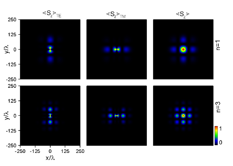
Figure 3: (Color online) Normalized energy fluxes $\langle S_{z}\rangle_{TE}$, $\langle S_{z}\rangle_{TM}$ and $\langle S_{z}\rangle$ of the FPGB with beam order $n=1$ and $n=3$ (from top to bottom) in the reference plane $z=2000\lambda$, respectively. Waist size $w_{0}$ is set to $10\lambda$, and the circular aperture radius $R\rightarrow\infty$.

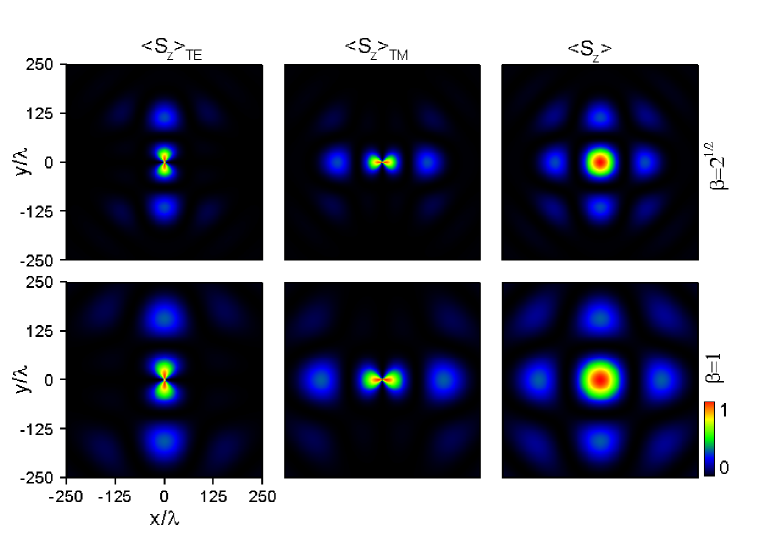
Figure 4: (Color online) Normalized energy fluxes $\langle S_{z}\rangle_{TE}$, $\langle S_{z}\rangle_{TM}$ and $\langle S_{z}\rangle$ of the hard-edged-diffracted four-petal Gaussian beam with beam order $n=1$ in the reference plane $z=2000\lambda$. The truncation parameter is set to $\beta=\sqrt{2}$ and $\beta=1$(from top to bottom), respectively. Waist size $w_{0}$ is set to $10\lambda$.

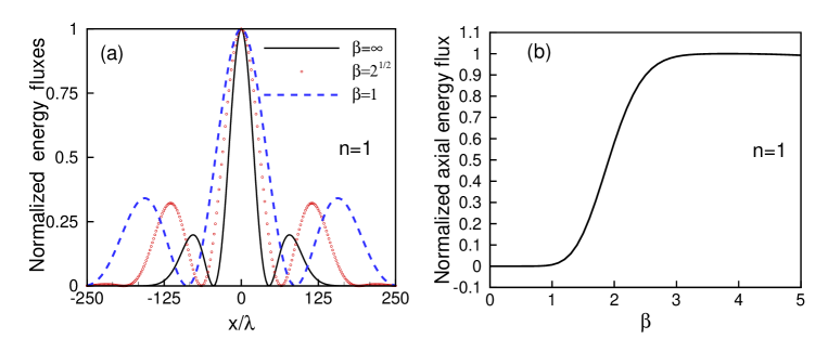
Figure 5: (Color online) Cross section and on-axis value of the normalized total energy flux of the hard-edged-diffracted four-petal Gaussian beam with the beam order $n=1$ in the reference plane $z=2000\lambda$. Waist size $w_{0}$ is set to $10\lambda$. (a) The cross section with respect to x direction ($y=0$) with various truncation parameter $\beta=1$(dashed curve), $\beta=\sqrt{2}$(circled curve), and $\beta=\infty$(solid curve), respectively, (b) Normalized axial energy flux at $z=2000\lambda$ versus the truncation parameter $\beta$.

The influence of the diffraction effect introduced by the aperture on the energy flux distributions of the four-petal Gaussian beam is depicted in Fig. 4 and Fig. 5 based on Eqs. (30)$-$ (32). Waist size $w_{0}$ is set to $10\lambda$. For simplicity, the beam order $n$ is set to be $1$. In Fig. 4, the truncation parameter is set to $\beta=\sqrt{2}$ and $\beta=1$, respectively. According to Eq.(3), the four peak-value positions of the incident beam is just on the boundary line of the circle when the truncation parameter is set to $\beta=\sqrt{2}$ for $n=1$. Comparing top subfigure of Fig. 3 with Fig. 4, one can find that central spot and side lobes spread more widely in the far field when the circular aperture exists. Moreover, the smaller radius of the aperture is, the more wide distribution of the energy flux is. This phenomenon is easy to understand because the initial field is confined by the aperture and its diffracted field has bigger divergence angle in the far field [23]. For the sake of showing clearly, cross section and on-axis value of the whole energy flux is plotted based on Eq. (32) in Fig. 5. Fig. 5(a) shows cross section of the total energy flux at $y=0$ for different truncation parameter, from which we can see clearly that the relative values of the lobes and the full width at half maximum (FWHM) of central spot become bigger when the truncation parameter decreases. The values of FWHM are $41.6\lambda$ for $R=\infty$, $61.8\lambda$ for $\beta=\sqrt{2}$, and $83.8\lambda$ for $\beta=1$, respectively. In addition, the ratios of the maximum value of the first side-lobe to that of the central spot are $0.19$ for $\beta=\infty$, $0.32$ for $\beta=\sqrt{2}$, and $0.34$ for $\beta=1$, respectively. The on-axis energy flux of the whole beam at $z=2000\lambda$ versus truncation parameter $\beta$ is shown in Fig. 5(b). It should be noticed that truncation parameter cannot be too small in order to obtain the better transmissivity in practical application.

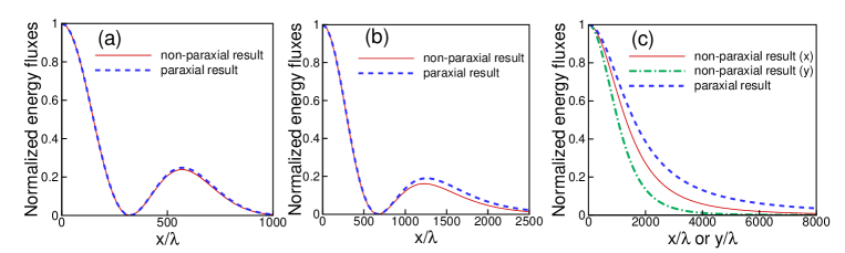
Figure 6: (Color online) Cross section at $y=0$ of the normalized total energy flux of the hard-edged-diffracted four-petal Gaussian beam with the beam order $n=1$ in the reference plane $z=2000\lambda$. The solid and the dashed curves denote the non-paraxial and the paraxial results, respectively. Truncation parameter $\beta$ is 2. In subfigure(c) cross section at $x=0$ is also plotted based on non-paraxial result. (a) $f=0.1$, (b) $f=0.2$, (c) $f=1.5$.

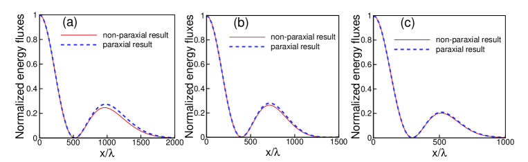
Figure 7: (Color online) Cross section at $y=0$ of the normalized total energy flux of the hard-edged-diffracted four-petal Gaussian beam with the beam order $n=1$ in the reference plane $z=2000\lambda$. The solid and the dashed curves denote the non-paraxial and the paraxial results, respectively. The f-parameter is set to be 0.1. (a) $\beta=1.1$, (b) $\beta=1.5$, (c) $\beta=2.5$.

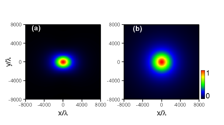
Figure 8: (Color online) Normalized total energy flux of the hard-edged-diffracted four-petal Gaussian beam with the beam order $n=1$ in the reference plane $z=2000\lambda$. The $f$-parameter is set to be 1.5. $\beta=2.0$. (a) non-paraxial result, (b) paraxial result.

It is well known that the paraxial approximation is allowable when $w_{0}/\lambda$ is much larger than 1. The far field expression of the four-petal Gaussian beam diffracted by a circular aperture under paraxial regime can be treated as a special case by using approximation

$$r=z+\frac{\rho^{2}}{2z}\approx z.$$ (37)

Therefore, the paraxial expression of the whole energy flux of the four-petal Gaussian beam diffracted by a circular aperture turns out to be

$$\langle S_{z}\rangle=\frac{1}{2}\sqrt{\frac{\varepsilon}{\mu}}\frac{G_{n}^{2}Z_{R}^{2}}{\pi^{2}}\frac{1}{r^{2}}\left[\Gamma(n+\frac{1}{2})\right]^{4}\mid S_{n}(x,y,z,f,\beta)\mid^{2}.$$ (38)

Eq. (38) is symmetric about the x and y variables, whereas Eq. (32) is somewhat asymmetric about the x and y variables. With the given beam order, the non-paraxiality of an apertured FPGB depends on $f$-parameter and truncation parameter $\beta$. Fig. 6 shows cross section at $y=0$ of the normalized total energy flux of the hard-edged-diffracted four-petal Gaussian beam with different $f$-parameter in the reference plane $z=2000\lambda$. Truncation parameter $\beta$ is 2. For simplicity, the beam order $n=1$(hereafter). The solid and the dashed curves denote the non-paraxial and the paraxial results, respectively(hereafter). From Fig. 6(a) one find that the difference between the non-paraxial and the paraxial results is negligible for $\beta=2$ and $f\leq 1$. The difference between them becomes evident as $f$-parameter increases. The central beam spot obtained by paraxial result is obviously larger than that obtained by non-paraxial result and side lobes disappear when $f$-parameter increases enough, which is shown in Fig. 6(c). Moreover, the cross section at $x=0$ is also plotted in Fig. 6(c) in order to observe the asymmetry. Fig. 7 shows cross section at $y=0$ of the normalized total energy flux of the hard-edged-diffracted four-petal Gaussian beam with different truncation parameter in the reference plane $z=2000\lambda$. The $f$-parameter is 0.1. The difference between paraxial result and non-paraxial result becomes evident as truncation parameter decreases. Comparing Fig. 6 with Fig. 7, we obtained a conclusion that the $f$-parameter plays a more key role in determining the non-paraxiality of an apertured FPGB than does the truncation parameter $\beta$, which is similar to the conclusions of Ref. [24, 25]. In order to understand, Fig. 6(c) are plotted in contour graphs, which is shown in Fig. 8. It can be clearly shown the non-paraxial result is approximately elliptic, which is obviously different from the paraxial result. The above conclusion is also applicable to other higher beam order.

5 Conclusions

In summary, the vectorial structure of an apertured four-petal Gaussian beam in the far field is derived in the analytical form by using the vector angular spectrum method, the complex Gaussian expansion of the circular aperture function, and the stationary phase method. Based on the analytical vectorial structure of an apertured beam, the energy flux distributions of the TE term, the TM term and the whole beam are derived in the far-field. Our formulas obtained in this paper are applicable to both non-paraxial case and paraxial case. When the truncation parameter $\beta$ tends to infinity, our formulas degenerate into the un-apertured case. The four-petal Gaussian beam cannot preserve its initial shape, and the number of petals in the far field gradually increases when beam order $n$ increases. Energy distributions spread more widely in the far field when the circular aperture exists. The influence of $f$-parameter and truncation parameter on the far-field behavior is also studied in detail. The $f$-parameter plays a more key role in determining the non-paraxiality of an apertured FPGB than does the truncation parameter $\beta$. In addition, the asymmetry of beam spot becomes apparently with increasing non-paraxiality. This work is important to understand the theoretical aspects of vector FPGB and is beneficial to its practical appliction.

References

[1]
M. Reicherter, T. Haist, E.U. Wagemann, H.J. Tiziani, Opt. Lett.
24 (1999) 608.