Ultrafast Cascading Theory of Intersystem Crossings in Transition-Metal Complexes

Abstract

We investigate the cascade decay mechanism for ultrafast intersystem crossing mediated by the spin-orbit coupling in transition-metal complexes. A quantum-mechanical description of the cascading process that occurs after photoexcitation is presented. The conditions for ultrafast cascading are given, which relate the energy difference between the levels in the cascading process to the electron-phonon self energy. These limitations aid in the determination of the cascade path. For Fe²⁺ spin-crossover complexes, this leads to the conclusion that the ultrafast decay primarily occurs in the manifold of antibonding metal-to-ligand charge-transfer states. We also give an interpretation for why some intermediate states are bypassed.

I Introduction

Cascade decay is a universal phenomenon associated with excited-state relaxation in photophysics and photochemistry. In most materials, the excited state that is reached after photoexcitation does not directly decay to the ground state but follows a complex route of intermediate states with often surprising changes in, e.g., spin and lattice parameters. The fastest cascading effects are generally associated with dephasing of states through the coupling to a continuum, e.g. Fano effects.Fano After the cascade, the system returns to the ground state or to a relatively long-lived metastable state. A highly complex example of cascading is photosynthetic water oxidation where multiple photoexcitations of a Mn₄Ca complex bound to amino acid residues in photosystem II leads to the production of O₂ from water molecules.Dau Obviously, a theoretical quantum-mechanical treatment of cascading is of the upmost importance but is also highly complex, and even many simpler systems are not well understood. A prototypical example of cascading occurs in spin-crossover phenomena in transition-metal complexes where photoexcitation of a low-spin ground state can lead to the creation of high-spin configurations on timescales as fast as several hundreds of femtosecond (fs). The reverse process has also been observed. Probably, the best-studied examples are Fe²⁺ complexes with a singlet $t_{2g}^{6}$ ground state (${}^{1}A_{1}$ in $O_{h}$ symmetry) and a high-spin $t_{2g}^{4}e_{g}^{2}$ (${}^{5}T_{2}$) configuration.Decurtins ; Gawelda1 ; Gutlich1 ; Hauser ; Bressler ; McCusker ; Gawelda2 ; Ogawa ; Kirk ; Forster The relaxation from the metastable high-spin state to the ground state is slow with decay times ranging from nanoseconds to days.

The advantage of studying the intersystem crossing in Fe compounds is that the cascading clearly involves two subsequent $t_{2g\downarrow}\rightarrow e_{g\uparrow}$ conversions. That this leads to an increase in the metal-ligand distance is well known since electrons in $e_{g}$ orbitals repel the ligands more strongly than those in the $t_{2g}$ orbitals. However, our understanding is complicated by the fact that excitations are not made into the local $dd$ multiplets, which are generally well understood by ab initio techniques in the adiabatic limit,Suaud ; Ordejon but into the metal-to-ligand charge-transfer states. This makes the exact nature of the cascade path difficult to understand due to the competition between internal conversion between states of the same spin and intersystem crossings between states with different spin. Generally, the latter process is considered slower than the former. Furthermore, the decay is a nonadiabatic process requiring the relaxation of oscillations of vibronic states. This intramolecular vibrational energy redistribution is considered the fastest process.

In this paper, we first provide a quantum-mechanical cascade decay model for the photoinduced electron state in transition-metal complexes. A dissipative Schrödinger equation is introduced to include the effects of the interaction with the surroundings. In the case of Fe spin-crossover complexes, we propose a novel and selfconsistent photon-excited decay path, and find the cascade decay times in good agreement with experiments on the order hundreds of femtoseconds from the photoexcited singlet state to the quintet state. Although our decay times are in qualitative agreement with that of phenomenological rate equations, the more detailed understanding of the cascading allows a better identification of the states involved in the decay path and their time-dependent occupation than is possible with rate equations with constants inferred from experimental data.Hauser ; Forster

II cascade decay Model

In a cascading process, several levels at energies $E_{i}$ are involved. The levels couple to the vibrational/phonon modes of energy $\hbar\omega$ of the surrounding ligands. Variations in coupling strength $\lambda_{i}$ lead to different metal-ligand equilibrium distances for different states. The Hamiltonian is given by

$$H_{s}=\sum_{i}E_{i}n_{i}+\hbar\omega a^{\dagger}a+\lambda_{i}n_{i}\left(a^{\dagger}+a\right),$$ (1)

where $n_{i}$ gives the occupation of state $i$ and $a^{\dagger}$ is the step operator for the vibrational mode. This Hamiltonian can be diagonalized with a unitary transformation $\bar{H_{s}}=e^{S}H_{s}e^{-S}$, with $S=\sum_{i}n_{i}\sqrt{g_{i}}\left(a^{\dagger}-a\right)$ and $g_{i}=\varepsilon_{i}/\hbar\omega$ with $\varepsilon_{i}=\lambda_{i}^{2}/(\hbar\omega)$, giving,

$$\bar{H_{s}}=\sum_{i}\left(E_{i}-\varepsilon_{i}\right)n_{i}+\hbar\omega a^{\dagger}a.$$ (2)

with eigenstates $|\psi_{in}\rangle$ for states $i$ and $n$ excited phonon modes. We define the energy difference between the states after diagonalization $\Delta_{ij}=\left(E_{i}-\varepsilon_{i}\right)-\left(E_{j}-\varepsilon_{j}\right)$. In addition, since a spatial translation of the coordinates shifts all the $\lambda_{i}$ by a constant in $H_{s}$, only the relative change in coupling is of importance. Therefore, it is useful to define the electron-phonon self-energy difference $\varepsilon_{ij}=\left(\lambda_{i}-\lambda_{j}\right)^{2}/(\hbar\omega)$ between two different states (as shown in right panel of Fig. 1). An interaction that cannot be diagonalized with the electron-phonon term is the spin-orbit coupling, which explains the prevalence of spin-flips in many decay processes. This causes a coupling between different states,

$$H_{I} = \sum_{ij}V_{ij}(c_{i}^{\dagger}c_{j}+{\rm h.c.}),$$ (3)

where $V_{ij}$ is the coupling constant and $c_{i}^{\dagger}c_{j}$ causes a particle-conserving transition between states $j$ and $i$. This ”local” system is considered part of a larger system such as a molecule in solution or a solid. The latter constitute the effective surroundings that can dissipate energy from the local system. In the following, we demonstrate how to incorporate electronic and vibronic dissipation.

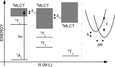
Figure 1: Left plane: Schematic energy level scheme of Fe²⁺-based complexes. The different configurations are given in octahedral notation. Manifolds of the metal-to-ligand charge-transfer (MLCT) states are indicated by the shadowed areas. Right plane: $\Delta$, $\varepsilon$ and $\Delta R$ are the energy gap between the lowest vibrational levels, the electron-phonon self-energy difference, and the change of the equilibrium distance between two oscillation states, respectively.

III Environmental dissipation

The study of the dynamics of dissipative systems is notoriously difficult due to the absence of conservation of energy and/or particle number in local system and the complex interaction with the environment. The density matrix method is a standard approach to dissipation problems.Lin However, the density matrices may become unphysical under the perturbative expansion with respect to the system-bath coupling.Palmieri Although Lindblad equations can solve this problem,Lindblad a more serious disadvantage of the density-matrix technique is the difficulty in handling large systems. To reduce the calculation, a methodology that directly describes the nonequilibrium dynamics of the wavefunction is advantageous. For example, Strunz demonstrated that the dynamics of an open quantum system can be described by a non-Markovian stochastic Schrödinger equation.Strunz Here, we describe a open quantum system with a dissipative Schrödinger equation for the system state $|\psi(t)\rangle$ which is given by

$$i\hbar\frac{d|\psi(t)\rangle}{dt}=\left(H_{0}+iD\right)|\psi(t)\rangle,$$ (4)

where $H_{0}$ is the Hamiltonian of the system and $D$ describes the effective environmental dissipation.

When selecting the basis, we write the system vector,

$$|\psi(t)\rangle=\sum_{k}c_{k}(t)|\psi_{k}\rangle,$$ (5)

with the coefficient $c_{k}$ in terms of an amplitude $a_{k}(t)=|c_{k}(t)|$ and a phase $\varphi_{k}$, or $c_{k}(t)=a_{k}(t)e^{i\varphi_{k}(t)}$. We can express the change in the coefficient due to the presence of the bath

$$\left.\frac{dc_{k}(t)}{dt}\right|_{B}=\left.\frac{da_{k}(t)}{dt}\right|_{B}e^{i\varphi_{k}(t)}+i\left.a_{k}(t)e^{i\varphi_{k}(t)}\frac{d{\varphi_{k}(t)}}{dt}\right|_{B}.$$ (6)

In general, the coupling to the environment affects both the probability and the phase of the system. The latter term gives the change in phase, which causes an embedding of the local system in its surroundings. Due to the complexity of the surroundings, the precise nature of this embedding is often very difficult and can usually only be taken into account in some effective way. Here, we assume that the phase of the local system is changed randomly by the large number of degrees of freedom of the surroundings which results in a total phase change close to zero according to the law of large numbers. We therefore only consider the changes in the probability by the environment. Now let us assume for the moment that we are able to determine an expression for the change in amplitude $P_{k}=a_{k}^{2}$ in a particular basis (e.g in the absence of certain intersystem couplings)

$$\left.\frac{dP_{k}}{dt}\right|_{B}=2a_{k}\left.\frac{da_{k}}{dt}\right|_{B}=f(\{P_{k}\}),$$ (7)

where $f$ is a function of the probabilities $P_{k}$. Below we give the explicit expression for the change in probabilities related to the damping of phonons. The change in the coefficient due to the bath is then given by

$$\left.\frac{dc_{k}}{dt}\right|_{B}=\frac{1}{2a_{k}}\left.\frac{dP_{k}}{dt}\right|_{B}e^{i\varphi_{k}}=\left.\frac{1}{2}\frac{d\ln P_{k}}{dt}\right|_{B}c_{k}.$$ (8)

This leads to a dissipative term in Eq. (4) given by

$$D=\frac{\hbar}{2}\sum_{k}\frac{d\ln P_{k}(t)}{dt}|\psi_{k}\rangle\langle\psi_{k}|.$$ (9)

The dissipation does not necessarily have to be diagonal. After deriving the diagonal dissipation in a particular basis, a unitary transformation to a different (more suitable) basis can be made. After deriving an expression for the dissipation in a particular basis set, we can solve the problem in the presence of intersystem couplings and dissipation.

In cascade decay model, the eigenvectors $|\psi_{in}\rangle$ of $\bar{H}_{s}$ are selected as the basis. The vibrational cooling by the bath can be taken into account by the dissipative Schrödinger equation in Eq. (4) with $H_{0}$ substituted by $\bar{H}_{s}+\bar{H}_{I}$ and $\bar{H}_{I}=e^{S}H_{I}e^{-S}$. We still need the detailed formulae for Eq. (7). For state $i$ with $n$ excited phonon modes, on the one hand, the vibrational coupling to the surroundings relaxes a state with $n$ phonons to a $n-1$ phonon state by the emission of phonons. On the other hand, the probability of the $n$-phonon state increases due to the decay of the state with $n+1$ phonons.Veenendaal ; Bopp This gives a change in the probability of the $n$-phonon state

$$\frac{dP_{in}(t)}{dt}=-2n\Gamma P_{in}(t)+2(n+1)\Gamma P_{i,n+1},$$ (10)

where $P_{in}(t)=\left|\left\langle\psi_{in}\right|\left.\psi(t)\right\rangle\right|^{2}$, $\Gamma=\pi\bar{\rho}\bar{V}^{2}/\hbar$ is the relaxation constant, where $\bar{\rho}$ is the effective bath phonon density of states and $\bar{V}$ is the interaction between the local system and the bath. Due to the complication of $\bar{V}$, we take $\Gamma$ as a parameter. Note that the decay time from state $i$ to $j$ is not directly related to $\Gamma$. Our numerical calculations are not sensitive to the change in $(2\Gamma)^{-1}$ from 20 fs to 60 fs. In Figs. 2 and 3, we take $(2\Gamma)^{-1}=30$ fs.

IV iron spin-crossover complexes

Let us specifically consider iron-based complexes, such as Fe²⁺(bpy)₃. A typical energy level scheme is shown in Fig. 1. The Fe $d^{6}$ multiplet levels have been extensively studied. However, since these excitations are dipole forbidden, the system is often excited into so-called metal-to-ligand charge-transfer (MLCT) states. Spin crossovers are generally strongly covalent, where the metal states are given by $\alpha|d^{6}\rangle+\sum_{i}(\beta_{i}|d^{7}{\underline{L}}_{i}\rangle+\gamma_{i}|d^{5}L_{i}\rangle)+\cdots$, where $L_{i}$ and ${\underline{L}}_{i}$ are an electron and a hole, respectively, on the ligand labeled $i$. The MLCT states are the antibonding states related to the metal states (e.g. ¹MLCT$-^{1}$A₁,³MLCT$-^{3}$T_1,2 and ⁵MLCT$-^{5}$T₂). Since the photoexcitation conserves spin, the initial photoexcited state starting from a ${}^{1}A_{1}$ ground state is the ¹MLCT state (with predominantly $t_{2g}^{5}L^{1}$ character). A major problem in the identification of the states in the cascading process is that optical selection rules make it impossible to directly probe the intermediate states spectroscopically, and several cascading paths to the metastable high-spin ${}^{5}T_{2}$ configuration have been proposed. McCusker et al. McCusker suggested that the ¹MLCT state directly decays to the high-spin ${}^{5}T_{2}$ quintet state requiring a spin change of $\Delta S=2$. Gawelda et al. Gawelda2 proposed that the ¹MLCT state relaxes to the ³MLCT within 30 fs followed by a departure from this state within $\sim$120 fs. Subsequently, the quintet state is reached via intermediate ligand-field multiplets. Recently, Bressler et al. Bressler claimed that the ³MLCT ($t_{2g}^{4}e_{g}^{1}L^{1}$) state directly relaxes to the ${}^{5}T_{2}$ state bypassing the ligand field triplet state. It is surprising that several states are bypassed, such as the triplet states ${}^{3}T_{1,2}$, which are located between the ³MLCT and ${}^{5}T_{2}$, and that there is no ³MLCT to ${}^{3}T_{1,2}$ internal conversion, which is expected to occur on a faster timescale than the spin-crossover process.

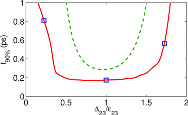
Figure 2: (color online) The time $t_{90\%}$ for the third state reaching its 90% population as a function of the energy difference between state 2 and 3 with $\Delta_{12}=\varepsilon_{12}=0.2$ eV and $\varepsilon_{23}=0.4$ eV. The solid (red) curve is calculated using the dissipative Schrödinger equation, the dashed (green) curve is based on rate equations with $t_{90\%}=-\ln 0.1/\gamma_{0}$ with $\gamma_{0}=\gamma_{1}\gamma_{2}/(\gamma_{1}+\gamma_{2})$, $\gamma_{1,2}$ are defined in Eq. 12. For the values of $\Delta_{23}$ indicated by the squares, the time dependence is given in Fig. 3.

In order to understand the cascade process in Fe-compounds, we first need to establish an appropriate range of parameters for Fe spin-crossover compounds. The strength of the interaction between the iron and its surrounding ligands can be obtained from ab initio calculations.Ordejon The change in energy for different configurations is close to parabolic for an adiabatic change in the Fe-ligand distance. From the change in equilibrium distance, we can obtain a difference in electron-phonon coupling $\varepsilon_{ij}$ of approximately $\varepsilon_{12}=0.2$ eV between the singlet and triplet state, and $\varepsilon_{23}=0.4$ eV between the triplet and quintet state. A typical energy for the Fe-ligand stretching mode is $\hbar\omega=$ 30 meV.Tuchagues Next, we need to determine the energies of the states involved in the cascading process. Since electronic transitions do not directly change the metal-ligand distance, an estimate of 2.6 eV can be obtained for the energy difference between the lowest vibrational levels of the ¹MCLT and ${}^{1}A_{1}$ states from the pump laser wavelength of 400 nm and the fluorescence of 600 nm from the lowest ¹MCLT state back to the ${}^{1}A_{1}$ state. Another weaker emission shows a shift to 660 nm corresponding to a change in energy of $\Delta_{12}=0.2$ eV.Gawelda2 This small energy difference implies that state 2 is a ³MLCT state,Gawelda2 see Fig. 1. For the spin-orbit coupling, we take the atomic value for Fe, $V_{12}=V_{23}=0.05$ eV.

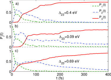
Figure 3: (color online) The probability of finding a particular state as a function of time for different values of $\Delta_{23}$. The green dashed-dotted, the blue dashed, and the red solid curves give the probability of finding states 1, 2, and 3, respectively: a) $\Delta_{23}=0.4$ eV; (b) $\Delta_{23}=0.09$ eV; (c) $\Delta_{23}=0.69$ eV. Other parameters are the same as those in Fig. 2.

This leaves us with the question of the nature of the third state and how a complete relaxation to the lattice parameters of the quintet state can be observed within 300 fs. We can obtain more information on the energy of the level in the cascading process by solving the cascading equations given above for cascading from level 1 to level 3 via an intermediate level 2. We define $i$ state occupation $P_{i}(t)=\sum_{n}P_{in}(t)$. Figure 2 shows the results for $t_{90\%}$, i.e., the time when the third level reaches its 90% population, as a function of $\Delta_{23}$. The value of $t_{90\%}$ shows a broad minimum around $\Delta_{23}\cong\varepsilon_{23}\cong 0.4$ eV. The minimum calculated time to reach a 90% occupation of the third level in the cascading process is about 200 fs. This is in good agreement with the results by Bressler et al. Bressler that show that the metal-ligand distance reaches the high-spin value on the same timescale. Let us first note that $t_{90\%}$ increases rapidly when $\Delta_{23}$ is less than $0.3\varepsilon_{23}\cong 0.12$ eV or larger than $1.7\varepsilon_{23}\cong 0.68$ eV. This implies that the total energy bridged in the fast cascading process is at most $\Delta_{12}+\Delta_{23}\cong 0.32$-0.88 eV. This is insufficient to overcome the more than 1.8 eV energy gap between the initial photoexcited state and the ${}^{5}T_{2}$ high-spin state. Another possibility is that an internal conversion occurs between states 2 and 3, for example, state 3 is a metal-centered ${}^{3}T_{1,2}$ triplet state, which are about 1 eV below state 2. For an internal conversion, the electron number of $e_{g}$ orbitals is unchanged, and $\varepsilon_{23}$ has to be less than $\varepsilon_{12}$ which does involve a $t_{2g\uparrow}\rightarrow e_{g\downarrow}$ conversion. Using a reduced electron-phonon self-energy of $\varepsilon_{23}$ of 0.2 eV while keeping $V_{23}=0.05$ eV, comparable results are obtained for the cascade time as a function of $\Delta_{23}/\varepsilon_{23}$ as in Fig. 2 (not shown). In order for the decay to occur in less than a picosecond, the energy gap between states 2 and 3 has to be less than $\mathopen{\sim}2\varepsilon_{23}=0.4$ eV. Therefore, even though the energy gap for an internal conversion is smaller, so is the maximum energy difference for which we can have ultrafast decay, and can also rule out the metal-centered triplet states as the third state in the cascading process. This is in agreement with experiment, since the metal-ligand separation increases to 0.2 Å Bressler showing that the high-spin state is reached. Furthermore, many internal conversion processes are also bypassed. Since the ligands $\pi^{*}$ orbitals are almost orthogonal to the metal $e_{g}$ orbitals, the electrons at the ligand atoms can only return to the $t_{2g}$ orbital. Therefore, this prohibits, for example, decay from the ¹MLCT ($t_{2g}^{5}L^{1}$) to the ${}^{1}T_{1}$ state ($t_{2g}^{5}e_{g}^{1}$). The only remaining possibility is that state 3 is a ⁵MLCT ($t_{2g}^{3}e_{g}^{2}L^{1}$) state. Furthermore, in the broad ⁵MLCT manifold, it is easier to find a level with $\Delta_{23}\approx\varepsilon_{23}$. This leads to the interesting conclusion that the entire ultrafast decay process occurs primarily in the antibonding MLCT states, a possibility not considered before. Subsequently, the ⁵MLCT state can relax more slowly to the ${}^{5}T_{2}$ state through internal conversion, which is difficult to observe in EXAFS experiments Bressler due to the comparable lattice parameters for the quintet states. This relaxation is slower since the spin-orbit coupling does not couple the two quintet states. Another reason that the ultrafast decay occurs in the MLCT states is that the broad manifold of MLCT states makes it easier to find states for which $\Delta_{ij}\approx\varepsilon_{ij}$, whereas for the ligand field multiplets, this condition is only satisfied accidentally. Therefore, for the first step in the cascade decay, it is not a coincidence that the strongest increase in intensity in the fluorescence occurs at $\Delta_{12}\approx 0.2$ eV,Gawelda2 close to the value of $\varepsilon_{12}$ although the energy of ³MLCT manifold spans over 1.5 eV.

A qualitative understanding of the time dependence of the decay can be obtained starting from classical phenomenological rate equations,Hauser ; Forster

$$\frac{dP_{i}(t)}{dt}=\gamma_{i-1}P_{i-1}(t)-\gamma_{i}P_{i}(t),$$ (11)

where $P_{i}(t)$ is the probability of $i$th level with $i=1...N$. The rate constants $\gamma_{i}$ can be calculated using Fermi’s golden rule,Bredas ; Schmidt

$$\gamma_{i}=2\pi F_{n}V_{i,i+1}^{2}/\hbar^{2}\omega,$$ (12)

where $V_{i,i+1}$ is the interaction between levels and $F_{n}=e^{-g}g^{n}/n!$ is the Franck-Condon factor with $n\approx\Delta_{i,i+1}/\hbar\omega$; $g=\varepsilon_{i,i+1}/\hbar\omega$ is the Huang-Rhys factor. Solving the above equations, we can approximately write the occupation of the final level in the cascading

$$P_{N}(t)\approx 1-e^{-\gamma_{0}t},$$ (13)

with $1/\gamma_{0}=\sum_{i=1}^{N-1}\left(1/\gamma_{i}\right)$. Figure 2 shows that, although rate equations give a qualitative description of $t_{90\%}$ as a function of $\Delta_{23}/\varepsilon_{23}$, quantitative differences are present. In the rate equation, energy conservation in Fermi’s Golden Rule restricts the relaxation to states of equal energy, whereas in the quantum mechanical calculation, the state couples to the whole Franck-Condon continuum. This leads to a smaller minimum value for $t_{90\%}$ and also to a significantly broader minimum for the quantum-mechanical cascading process. The broad width of the minimum somewhat loosens the condition $\Delta_{ij}\approx\varepsilon_{23}$, which further explains the prevalence of ultrafast-decay processes.

For $\Delta_{23}=0.4$ eV, we study the time-dependent occupations of the three states involved in the cascading process, see Fig. 3(a). We find that state 1 decays with a relaxation time about 20 fs. While the probability of state 2 increases quickly in the first 20 fs, it then begins to decrease due to relaxation into state 3. At 120 fs, it has lost most of its population, which agrees well with the experimentally observed departure from this state within $\sim$120 fs.Gawelda2 State 3 reaches almost 100% within 300 fs. All these timescales agree well with experiments.Bressler ; Gawelda2 For $\Delta_{23}=0.09$ eV and 0.69 eV, see Fig. 3(b) and (c), the decay of state 1 is almost the same as for $\Delta_{23}=0.4$ eV, since the decay from $1\rightarrow 2$ has been left unchanged, but the decay from state 2 has slowed down dramatically.

V Conclusions

In conclusion, we have provided a quantum-mechanical model for the cascade decay mechanism of spin crossover in transition-metal complexes. Ultrafast cascading occurs when the energy difference between the levels is comparable to the self energy $\varepsilon$. Since the latter is on the order of several tenths of an electronvolt, restrictions are imposed on the energy gap that can be bridged in the ultrafast cascading process. On the other hand, the manifold of the metal-to-ligand charge-transfer states make the gaps between energy levels many and various. As a result, the ultrafast cascading in Fe spin-crossover complexes after excitation with visible light occurs primarily in these manifolds. We propose a novel and selfconsistent photon-excited decay path for [Fe${}^{\text{II}}$(bpy)₃]²⁺, which is then ¹MLCT$\rightarrow^{3}$MLCT$\rightarrow^{5}$MLCT$\rightarrow^{5}$T${}_{2}\rightarrow^{1}$A₁. Good agreement is found between the calculated and experimentally observed decay times. Our quantum model results qualitatively agree with the calculation of decay times based on the phenomenological rate equations combining with Franck-Condo factor. We further give an explanation why some intermediate states are bypassed.

Acknowledgments. We are thankful to Xiaoyi Zhang and Yang Ding for helpful discussions. This work was supported by the U.S. Department of Energy (DOE),Office of Basic Energy Sciences, Division of Materials Sciences and Engineering under Award No. DE-FG02-03ER46097, and NIU’s Institute for Nanoscience, Engineering, and Technology. Work at Argonne National Laboratory was supported by the U.S. DOE, Office of Science, Office of Basic Energy Sciences, under Contract No. DE-AC02-06CH11357.

References

- (1) U. Fano, Phys. Rev. 124, 1866 (1961).
- (2) See e.g. H. Dau and M. Haumann, Coord. Chem. Rev. 252, 273 (2008).
- (3) S. Decurtins, P. Gütlich, K. M. Hasselbach, A. Hauser, and H. Spiering, Inorg. Chem. 24, 2174 (1985).
- (4) A. Hauser, J. Chem. Phys. 94, 2741 (1991).
- (5) J. K. McCusker, K. N. Walda, R.C. Dunn, J. D. Simon, D. Magde, and D. N. Hendrickson, J.Am.Chem.Soc. 115, 298 (1993).
- (6) P. Gütlich, A. Hauser, and H. Spiering, Angew. Chem. Int. Ed Engl. 33, 2024 (1994).
- (7) W. Gawelda, V.-T. Pham, M. Benfatto, Y. Zaushitsyn, M. Kaiser, D. Grolimund, S. L. Johnson, R. Abela, A. Hauser, C. Bressler, and M. Chergui, Phys. Rev. Lett. 98, 057401 (2007).
- (8) W. Gawelda, A. Cannizzo, V. Pham, F. van Mouik, C. Bressler, and M. Chergui, J. Am. Chem. Soc. 129, 8199 (2007).
- (9) Y. Ogawa, S. Koshihara, K. Koshino, T. Ogawa, C. Urano, and H. Takagi, Phys. Rev. Lett. 84, 3181 (2000).
- (10) Ch. Bressler, C. Milne, V.-T. Pham, A. ElNahhas, R. M. Van der Veen, W. Gawelda, S. Johnson, P. Beaud, D. Grolimund, M. Kaiser, C. N. Borca, G. Ingold, R. Abela, and M. Chergui, Science, 323,489 (2009).
- (11) A. D. Kirk, Chem. Rev. 99, 1607 (1999).
- (12) L. S. Forster, Coord. Chem. Rev. 227, 59 (2002).
- (13) N. Suaud, M.-L. Bonnet, C. Boilleau, P. Labéguerie, and N. Guihéry, J. Am. Chem. Soc. 131, 715 (2009).
- (14) B. Ordejón, C. de Graaf, and C. Sousa, J. Am. Chem. Soc. 130, 13961 (2008).
- (15) see e.g. S. H. Lin, R. Alden, R. Islampour, H. Ma, and A. A. Villaeys, Density Matrix Method and Femtosecond Processes (World Scientific, Singapore, 1991).
- (16) B. Palmieri, D. Abramavicius, and S. Mukamel, J. Chem. Phys. 130, 204512 (2009).
- (17) G. Lindblad, Commun. Math. Phys. 48, 119 (1976).
- (18) W.T. Strunz, Dynamics of Dissipation, Lecture Notes in Physics, Vol 597. Springer-Verlag, Berlin, 2006, p. 377.
- (19) F. Bopp, Sitzungsber. Math. Naturwiss. Kl. Bayer. Akad. Wiss. Muenchen 67, 122 (1973); H. Dekker, Phys. Rep. 80, 1 (1981).
- (20) M. van Veenendaal, J. Chang, and A. J. Fedro, Phys. Rev. Lett. 104, 067401 (2010); arXiv:1005.1079 (unpublished).
- (21) J. P. Tuchagues, A. Bousseksou, G. Molnár, J. J. McGarvey, and F. Varret, Top. Curr. Chem. 235, 85 (2004).
- (22) J.-L. Brédas et al. Chem. Rev. 104, 4971 (2004).
- (23) K. Schmidt et al., J. Phys. Chem. A 111, 10490 (2007).