Tunable Fano-Kondo resonance in side-coupled double quantum dot system

Abstract

We study the interference between the Fano and Kondo effects in a side-coupled double-quantum-dot system where one of the quantum dots couples to conduction electron bath while the other dot only side-couples to the first dot via antiferromagnetic (AF) spin exchange coupling. We apply both the perturbative renormalization group (RG) and numerical renormalization group (NRG) approaches to study the effect of AF coupling on the Fano lineshape in the conduction leads. With particle-hole symmetry, the AF exchange coupling competes with the Kondo effect and leads to a local spin-singlet ground state for arbitrary small coupling, so called “two-stage Kondo effect”. As a result, via NRG we find the spectral properties of the Fano lineshape in the tunneling density of states (TDOS) $\rho_{c}(\omega)$ of conduction electron leads shows double dip-peak features at the energy scale around the Kondo temperature and the one much below it, corresponding to the two-stage Kondo effect; it also shows an universal scaling behavior at very low energies. We find the qualitative agreement between the NRG and the perturbative RG approach. Relevance of our work to the experiments is discussed.

I. Introduction

Fano resonance is the quantum interference effect between a localized state with finite-width and a conduction bandfano . The hallmark of the Fano resonance is the asymmetric lineshape in tunnelling density of states (TDOS) of the conduction band. One example of Fano resonance is the transport through low dimensional electronic (Fermi) system with local impurities. The Kondo effectkondo plays an important role if these impurities carry unpaired spins. Recently, there has been growing interest both theoretically and experimentally in the Fano resonance associated with the Kondo effect via the STM measurements of noble metal surfacesxiang ; kroha ; schiller ; gadzuk ; wingreen ; schneider ; eigler as well as in quantum dot deviceshofstetter ; sato . The Fano resonance in these systems in general arises from two quantum interference effects: 1. between the broadened local level and the continuum conduction band and 2. between the Kondo resonance in the local level and the conduction band. The combined two effects give rise to rather complicated lineshpe in STM measurement of the TDOS. The Fano resonance in TDOS of conduction electrons in such systems can be served as an alternative approach to study the Kondo effect in addition to the local density of states of the quantum dot. The Fano lineshape in TDOS of conduction electrons in the leads of a single Kondo dot system has been extensively studied, and it is sensitive to both the spatial phase of the free conduction electrons and the scattering phase shift associated with the Kondo effect.

Very recently, the Fano resonance has been extended experimentallysasaki and theoreticallylee ; nishi to the side-coupled double quantum dot system where the competition between Kondo and Fano effects gives rise to change in conductance profile. In this paper, we investigate the Fano-Kondo interference in the side-coupled double-quantum-dot systems where only one of the two dots (dot $1$) connects to the leads while the other isolated dot (dot $2$) is side-coupled to dot $1$side ; grempel . In the Kondo limit where charging energy on each dot is large, an antiferromagnetic (AF) spin exchange (RKKY) coupling is generated via the second-order hoping between two dots competes with the Kondo effect, leading to local spin-singlet ground state for arbitrary finite values of $J$, so-called ”two-stage Kondo effect”side ; grempel . Previous studies on the side-coupled double-dot systems have been mostly focused on the dip of LDOS on dot $1$ upon applying the AF RKKY coupling. However, little is known about the feedback effect of the two-stage Kondo effect mentioned above on the TDOS of conduction electrons in the leads. In this paper, we generalize the Fano lineshape in TDOS of electrons in the leads as a result of the two-stage Kondo effect in side-coupled double-quantum-dot system. The systematic perturbative and numerical renormalization group approaches are applied here in the cases both with and without particle-hole symmetry. We find as a consequence of the two-stage Kondo effect, the spectral property of the Fano lineshape in TDOS of the leads develops an asymmetrical double dip/peak structure; it also shows an universal scaling behavior at very low energies. We compare our NRG results with the perturbative RG analysis.

II. The Model Hamiltonian.

Our starting Hamiltonian for the side-coupled double-dot system is the single-impurity Anderson model for dot $1$ with additional antiferromagnetic spin-exchange coupling between dot $1$ and the isolated dot $2$ which side-coupled to itside .

$$H = \sum_{k,\alpha=L,R}\epsilon_{k}c^{\dagger}_{k\alpha\sigma}c_{k\alpha\sigma}+\sum_{\alpha=L,R}\sum_{k,\sigma}(t_{\alpha}c^{\dagger}_{k\alpha\sigma}d_{1,\sigma}+h.c.)$$ (1)

$$+ \sum_{i\sigma}\epsilon_{di}d_{i\sigma}^{\dagger}d_{i\sigma}+\sum_{i=1,2}U_{i}n_{i}^{\uparrow}n_{i}^{\downarrow}$$

$$+ J\,{\bf S}_{1}\,{\bf S}_{2},$$

where $t_{L}$ and $t_{R}$ denote the tunneling amplitudes to the left and right leads, respectively, and $c^{\dagger}_{\alpha\epsilon\sigma}$ creates an electron in lead $\alpha=L,R$ with spin $\sigma$. This tunnel coupling leads to a broadening of the level on dot 1, the width of which is given by $\Gamma=\Gamma_{L}+\Gamma_{R}=2\pi(t_{L}^{2}\varrho_{L}+t_{R}^{2}\varrho_{R})$, with $\varrho_{L/R}$ the density of states in the leads. Here, $i=1,2$ labels the two dots, and ${\bf S}_{i}=(1/2)\sum_{\sigma\sigma^{\prime}}d_{i\sigma}^{\dagger}{\bf\sigma}_{\sigma\sigma^{\prime}}d_{i\sigma^{\prime}}^{{\phantom{\dagger}}}$ is their spin. Each dot is subject to a charging energy, $U_{1}\approx U_{2}=U=E_{C}$. In the presence of particle-hole symmetry, we have $\epsilon_{di}=-\frac{U_{i}}{2}$. Note that in the Kondo limit where the charging energy $E_{C}$ is large, the direct hoping between the two dots are strongly suppressed and an antiferromagnetic spin exchange coupling $J>0$ is generated via the second-order hoping processes.

The physical observables of our interest are: (i). LDOS of impurity on dot $1$: $\rho_{d1}(\omega)=\frac{-1}{\pi}ImG_{d1}(\omega)$ and (ii) the TDOS of the conduction electron $\rho_{c}(\omega)$: $\rho_{c}(\omega)=\rho_{0}+\delta\rho_{c}(\omega)$ where $\rho_{0}$ is the density of states of the bare conduction electron leads : $\rho_{0}=\frac{-1}{\pi}ImG_{c}^{0}(\omega=0)$ with $G_{c}^{0}(\omega-{\it i}\eta)$ being the bare conduction electron Green’s function, and $\delta\rho_{c}(\omega)$ is the correction to the LDOS of the conduction electron due to the coupling between leads and the quantum dot system: $\delta\rho_{c}(\omega)=\frac{-1}{\pi}Im\delta G_{c}(\omega-{{\it i}\eta})$. Here, the correction to the conduction electron Green’s function $\delta G_{c}(\omega-{\it i}\eta)$ is given by:

$$\delta G_{c}(\omega-{\it i}\eta)=\frac{\Gamma}{\pi\rho_{0}}G_{c}^{0}(\omega-{\it i}\eta)G_{d1}(\omega-{\it i}\eta)G_{c}^{0}(\omega-{\it i}\eta)$$ (2)

Using Eq. 2, we havekroha

$$\delta\rho_{c}(\omega)=-\Gamma\rho_{0}\times$$

$$[(q_{c}^{2}-1)ImG_{d1}(\omega-{\it i}\eta)-2q_{c}ReG_{d1}(\omega-{\it i}\eta)],$$ (3)

with $q_{c}$ being defined as

$$q_{c}=-\frac{ReG_{c}^{0}(\omega-{\it i}\eta)}{ImG_{c}^{0}(\omega-{\it i}\eta)},$$ (4)

and it can be treated approximately as an frequency-independent constant kroha ; xiang . Following Ref. side , below we apply both perturbative renormalization group (RG) and numerical renormalization group (NRG) approaches to calculate these quantities in the presence of particle-hole symmetry. Though the LDOS on dot $1$ (or equivalently the imaginary part of the Green’s function on dot $1$, $ImG_{d1}(\omega)$) at finite RKKY coupling $J$ via both RG and NRG has been computed in Ref. side , the real part of $G_{d1}(\omega)$, $ReG_{d1}(\omega)$, which is also needed to analyze the spectral property of the Fano lineshape in the TDOS of the conduction electron leads ($\rho_{c}(\omega)$), has not yet been calculated by either perturbative RG or NRG approach. In the following, we provide a numerical and analytical analysis on the Fano lineshape for $\rho_{c}(\omega)$ by analyzing both the real and the imaginary parts of $G_{d1}(\omega)$ at finite $J$ via NRG and compare them with those via perturbative RG approach.

First, we discuss the case for $J=0$. For $J=0$ and in the presence of particle-hole symmetry ($\epsilon_{di}=-U_{i}/2$), it has been known that in the Kondo regime $\omega\ll T_{k}$ with $T_{k}\approx D_{0}e^{-\pi\Gamma/U_{1}}$ being the Kondo temperature for dot $1$, $G_{d1}(\omega)$ is well approximated by the single Lorentzianside :

$$G_{d1}(\omega)\approx T_{d1}^{0}(\omega-{\it i}\eta)=\frac{z}{\omega+{\it i}\;\tilde{T}_{K}+{\it i}\eta}\;,$$ (5)

with $z=c\;\frac{T_{K}}{\Gamma}$ being the quasi-particle weight at the Fermi energy, and $\tilde{T}_{K}=z\Gamma=c\;T_{K}$ being an energy of the order of the Kondo temperature, $T_{K}$. The precise value of the universal constant $c$ relating $T_{K}$ and $\tilde{T}_{K}$ depends on the definition of $T_{K}$. Here, we define $T_{K}$ as the half-width of the transmission $T(\omega)\equiv-\Gamma ImG_{d1}(\omega)$. From fitting $G_{d1}(\omega)$ with the NRG data, we get $c\approx 0.5$. Note that by Fermi-liquid theory and principles of renormalization group, the RKKY interaction also gets renormalized by the same $z-$ factor: $J\rightarrow\frac{\tilde{J}}{z}$side . Here, $\tilde{J}$ is slightly different from $J$ due to the large logarithmic tail in $ImG_{d1}(\omega)$. The value of $\tilde{J}$ is obtained from the fit of $ImG_{d1}(\omega)$ to NRG data: $\tilde{J}\approx 1.1J$side . However, for $\omega\geq T_{k}$, the above simple Lorentzian approximation fails to account for the large logarithmic tail in $ImG_{d1}(\omega)$. Therefore, corrections to the single Lorentzian approximation are needed in this case to more accurately describe $G_{d1}(\omega)$. Via the Dyson equation approach, taking into account the interference between the Kondo resonance and the broadened impurity level, we obtain a more accurate description for the Green’s function of the dot $1$xiang :

$$G_{d1}(\omega)=G_{d1}^{0}(\omega)+G_{d1}^{0}(\omega)\tilde{T}_{d1}(\omega)G_{d1}^{0}(\omega)$$ (6)

where the bare Green’s function on dot $1$, $G_{d1}^{0}(\omega)$, describing a local impurity level with a level broadening $\Gamma$ and LDOS $\rho_{d0}\equiv\frac{-1}{\pi}ImG_{d1}^{0}(\omega=0)$, is given by:

$$G_{d1}^{0}=\frac{1-n/2}{\omega-\epsilon_{d1}+{\it i}\Gamma}+\frac{n/2}{\omega-\epsilon_{d1}-U_{1}+{\it i}\Gamma}$$ (7)

with $n=<n_{d1}^{\uparrow}+n_{d1}^{\downarrow}>$ being the average occupation number on dot $1$; and $\tilde{T}_{d1}(\omega)$ is the scattering $T-$matrix corresponding to the Kondo resonance, given approximately byxiang :

$$\tilde{T}_{d1}(\omega-{\it i}\eta)\approx\frac{be^{{\it i}2\delta}}{\omega-\epsilon_{K}+{\it i}\;\tilde{T}_{K}+{\it i}\eta}\;$$ (8)

with $b$ being a fitting parameter to be fitted with the NRG data for $ImG_{d1}(\omega)$. In the presence of particle-hole symmetry, we have $n=1$, $\epsilon_{K}=0$. Here, $\delta$ in Eq. 8 corresponds to the phase shift associated with the Kondo resonance scattering, and it gives $\delta=\pi/2$ in the case of particle-hole symmetry. By fitting Eq. 6 with the NRG data, we find $b\approx z/(\pi\rho_{d0})^{2}$, which is in good agreement with the known result: $-ImG_{d1}(\omega=0)=1/\Gamma$ for a single impurity Anderson modelkondo . In the Kondo regime ($\omega\ll T_{k}$ and $E_{c}\gg\Gamma$) of our system and for $J=0$, the bare Green’s function on dot $1$, $G_{d1}^{0}(\omega)$, are approximately given by: $ReG_{d1}^{0}(\omega)\approx 0$, $\frac{-ImG_{d1}^{0}(\omega)}{\pi}\approx\rho_{d0}$. The above approximations lead to the following approximated expressions for $G_{d1}(\omega)$ after including the interference between the Kondo resonance and the broadened impurity (dot $1$) level via Eq. 6:

$$ReG_{d1}(\omega) \approx (\pi\rho_{d0})^{2}\frac{b\omega}{\omega^{2}+\tilde{T}_{K}^{2}}$$

$$ImG_{d1}(\omega) \approx -\pi\rho_{d0}-(\pi\rho_{d0})^{2}\frac{b\tilde{T}_{K}}{\omega^{2}+\tilde{T}_{K}^{2}}$$ (9)

with $\rho_{d0}=-\frac{1}{\pi}ImG_{d1}^{0}(\omega=0)$ being the LDOS of dot $1$ at $\omega=0$. From Eq. 3 and Eq. 9, in the Kondo limit the correction to conduction electron density of states can therefore be expressed in terms of the well-known Fano lineshapexiang ; kroha :

$$\delta\rho_{c}(\omega,J=0)\approx\rho_{0}(\frac{q_{c}^{2}+2q_{c}\epsilon-1}{\epsilon^{2}+1}+\beta),$$ (10)

where $\epsilon=\frac{\omega-\epsilon_{K}}{\tilde{T}_{K}},\beta=\pi\rho_{d0}\Gamma(q_{c}^{2}-1)$. Note that in general the Dyson equation approach in Eq. 6 is also valid for both $\omega\ll T_{k}$ and $\omega\approx T_{k}$ in the presence of large particle-hole asymmetry: $|\epsilon_{d1}-\epsilon_{F}|\leq\Gamma$ (with $\epsilon_{F}$ being the Fermi energy of the leads) where the the interference between the Kondo and broadened impurity level plays an important role in $G_{d1}(\omega)$xiang .

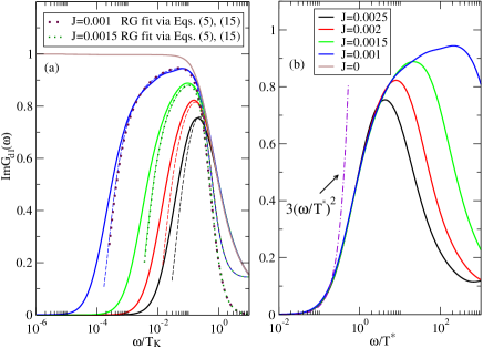
Figure 1: (a). $ImG_{d1}(\omega)$ (normalized to $ImG_{d1}(\omega=0,J=0)\approx-1/\Gamma$) of dot $1$ with particle-hole symmetry for different antiferromagnetic RKKY couplings $J$ calculated by NRG (solid lines) and perturbative RG (dashed lines) via Eqs. 6 and 15 (dashed lines). Dotted lines are RG fits via Eqs. 5 and 15. The NRG parameters are $U_{1}=U_{2}=D_{0}$, $\epsilon_{d1}=\epsilon_{d2}=-0.5D_{0}$, $\Gamma=0.2D_{0}$ with $D_{0}=1$. For $J=0$, we find $T_{k}\approx 0.005D_{0}$. The fitting parameters $c\approx 0.5$, and $\tilde{J}\approx 1.1$. (b). $ImG_{d1}(\omega/T^{*})$ (normalized to $ImG_{d1}(\omega=0,J=0)\approx-1/\Gamma$) shows an universal scaling behavior for $\omega<T^{*}$. The dot-dash line is the power-law $(\omega/T^{*})^{2}$ fit to the crossover function of $ImG_{d1}(\omega/T^{*})$ for $\omega\ll T^{*}$, see Eq. 17.

III. Perturbative Renormalization Group analysis

Now, we turn on a finite RKKY coupling $J$. Following Ref. side , to gain an analytical understanding we employing the perturbative renormalization group analysis in the limit of $J\rightarrow 0$. We restrict ourselves the case with particle-hole symmetry. Though some of the aspects in this case has been studied in Ref. side , it proves to be useful to summarize its key results for further calculations on the Fano lineshape for $\rho_{c}(\omega)$ in the presence of RKKY coupling $J$. In the limit $J\to 0$, “two-stage Kondo screening” takes placeside ; grempel : The spin of dot $1$ first gets Kondo screened below Kondo temperature $T_{K}\approx D\;e^{-\pi U/\Gamma}$ with $D$ being the bandwidth cutoff, the first stage Kondo effect. Then for energy scale much below $T_{k}$, the second stage Kondo effect occurs at $\omega<T^{*}\ll T_{k}$ between dot $1$ and $2$ via the antiferromagnetic RKKY coupling $J$ where the spin on the dot $2$ gets Kondo screened. Here, the Kondo resonance peak in electron density of states on dot $1$ plays the effective fermionic bath for the second stage Kondo effect. We will discuss how the Fano lineshape for $\rho_{c}(\omega)$ is affected in the presence of the antiferromagnetic RKKY coupling. Summing up all leading logarithmic vertex diagrams leads to the following scaling equation for the dimensionless vertex functionside

$$\frac{d(\gamma(\omega,\tilde{T_{k}}))}{dl}\equiv\frac{d(\hat{\varrho}(\omega)\tilde{J})}{dl}=({\hat{\varrho}}(\omega)\tilde{J})^{2}\;,$$ (11)

with the scaling variable defined as $l\equiv\log(\tilde{T}_{K}/\tilde{T}_{K}^{\prime})$. Here, $\hat{\varrho}(\omega)\equiv\varrho(\omega)/z=\frac{-1}{\pi z}ImG_{d1}(\omega)$ is the rescaled effective density of states of dot $1$. Integrating this differential equation up to $l\equiv\log(\tilde{T}_{K}/\omega)$, one obtains the dimensionless vertex function in the leading logarithmic approximationside :

$$\gamma(\omega,\tilde{T}_{K})=\frac{1}{\frac{\omega^{2}}{\tilde{T}_{K}^{2}}\log\frac{\tilde{T}_{K}}{T^{*}}+\log\frac{|\omega|}{T^{*}}}\;,$$ (12)

with the second scale $T^{*}$ defined as

$$T^{*}=\tilde{T}_{K}\;\exp(-\pi\;\tilde{T}_{K}/\tilde{J})\;.$$ (13)

The second order self-energy correction to the retarded Green’s function $G^{0}_{d1}$ simply gives the expressionside

$$\Sigma(\omega)=S(S+1)\frac{\tilde{J}^{2}}{4z^{2}}G_{d1}(\omega)$$ (14)

where S=1/2. The Green’s function of dot $1$ after including self-energy and vertex correction is given byside :

$$G^{J}_{d1}(\omega)=\frac{z}{zG_{d1}^{-1}(\omega)-\frac{\tilde{J}^{2}(\omega)S(S+1)}{4z}G_{d1}(\omega)}.$$ (15)

where $\tilde{J}(\omega)$ is replaced by $\gamma(\omega)/\hat{\varrho}(\omega)$, and $G_{d1}(\omega)$ is given by either Eq. 5 (the Dyson equation approach) or Eq. 6 (the single Lorentzian approximation). Note that due to the logarithmic corrections in $\gamma$, the spectral density of dot $1$ develops a dip at energies $\omega\sim T^{\ast}\ll T_{K}$ for any infinitesmall $J$, which suppresses the low-energy transmission coefficient through dot $1$. Physically, this comes from as a consequence of the fact that electrons of energy $\omega<T^{\ast}$ are not energetic enough to break up the local spin singlet and therefore their transport is suppressed. For a finite RKKY coupling $J>0$, the real and imaginary parts of $G_{d1}^{J}(\omega)$ obtained in Eq. 15 via perturbative RG approach lead to an analytical expression for the correction to the LDOS on dot $1$, $\delta\rho_{c}^{J}(\omega)$:

$$\delta\rho_{c}^{J}(\omega)=-\Gamma\rho_{0}[(q_{c}^{2}-1)ImG_{d1}^{J}(\omega)-2q_{c}ReG_{d1}^{J}(\omega)].$$ (16)

Below we present the results via NRG with fits by the perturbative RG calculations.

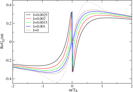
Figure 2: $ReG_{d1}(\omega)$ (normalized to $-ImG_{d1}(\omega=0,J=0)$) of dot $1$ for different antiferromagnetic RKKY couplings $J$ by NRG (solid lines). The dashed line is a fit to the NRG data for $J=0$ via Eq. 6. The other parameters are the same as in Fig. 1.

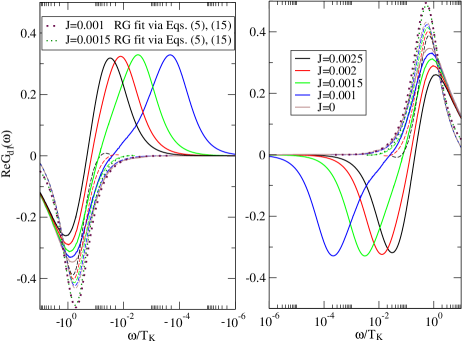
Figure 3: $ReG_{d1}(\omega)$ (normalized to $-ImG_{d1}(\omega=0,J=0)$) on a logarithmic scale of $\omega/T_{k}$ for different antiferromagnetic RKKY couplings $J$ by NRG (solid lines) and perturbative RG via Eqs. 6 and 15 (dashed lines). Dotted lines are RG fits via Eqs. 5 and 15. The other parameters are the same as in Fig1.

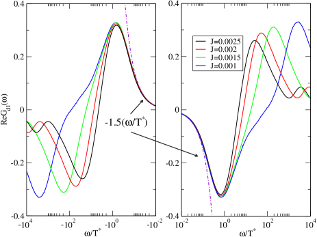
Figure 4: $ReG_{d1}(\omega)$ (normalized to $-ImG_{d1}(\omega=0,J=0)$) on a logarithmic scale of $\omega/T^{*}$ for different antiferromagnetic RKKY couplings $J$ by NRG. The other parameters are the same as in Fig. 1. The dot-dash lines are power-law $(\omega/T^{*})$ fits to the universal crossover function of $ReG_{d1}(\omega)$ for $\omega\ll T^{*}$, see Eq. 19.

IV. Comparison to the Numerical Renormalization Group (NRG) analysis.

We have performed the NRG calculations on the system in the presence of particle-hole symmetry. The NRG parameters we used are: $U_{1}=U_{2}=D_{0}=1$, $\epsilon_{d1}=\epsilon_{d2}=-0.5$, $\Lambda=2$, $\Gamma_{L}=\Gamma_{R}=0.1$ with $D_{0}$ being the bandwidth of the conduction electron baths. (Here, we set $D_{0}=1$ as the unit of all parameters.) Within each NRG iteration, we keep the lowest $1000$ states. For $J=0$, we find $T_{k}\approx 0.005D_{0}$. As RKKY coupling is increased, both real and imaginary parts of $G_{d1}(\omega)$ get splited at $\omega=0$. First, as shown in Ref. side , the imaginary part of $G_{d1}(\omega)$ (proportional to DOS of dot $1$) at finite $J$ shows a dip below the characteristic energy scale $T^{*}$ for any arbitrary $J>0$ (see Fig.1(a)). For small RKKY coupling $J$, the NRG results for $ImG_{d1}(\omega)$ can be fitted reasonably well by the perturbative RG approach over an intermediate energy range $T^{*}\ll\omega\ll T_{k}$. Furthermore, a clear universal scaling behavior of the KT type is observed from the NRG results of $ImG_{d1}(\omega)$ for $\omega\leq T^{*}$: $ImG_{d1}(\omega)\approx g_{0}g(\omega/T^{*})$ (see Fig. 1(b)) side . With particle-hole symmetry, the scaling function $g(\omega/T^{*})$ is completely universal. As pointed out in Ref. side , the ground state of the system at any finite $J$ is a local spin-singlet (a Fermi liquid), the very low energy crossover of $ImG_{d1}(\omega)$ for $\omega\ll T_{k}$ vanishes as $(\omega/T^{*})^{2}$, following the Fermi liquid behavior:

$$-\Gamma ImG_{d1}(\omega)\approx a_{1}(\frac{\omega}{T^{*}})^{2}.$$ (17)

where $a_{1}\approx 3.0$ from the fit to the NRG data (see Fig. 1 (b)) side . Note that we find the perturbative RG approach via Eq. 6 leads to a better fit to the NRG results for $ImG_{d1}(\omega)$ than that via Eq. 5, as expected.

We now discuss the real part of $G_{d1}(\omega)$. For $J=0$, $ReG_{d1}(\omega)$ is antisymmetric with respect to $\omega=0$ and it shows a peak/dip at $\omega\approx\pm T_{k}$, signature of the first Kondo effect. As the RKKY coupling $J$ is increased, the magnitude of the peak/dip in $ReG_{d1}(\omega)$ for $\omega\approx T_{k}$ decreases, indicating the Kondo effect is suppressed. At a much lower energy scale, $T^{*}\approx\omega\ll T_{k}$, the Kondo dip-peak structure in $ReG_{d1}(\omega)$ gets a further split with a width $D\approx 2T^{*}$: it develops a negative-valued dip for $\omega\approx T^{*}$; while it shows a positive-valued peak for $\omega\approx-T^{*}$. In the $\omega\rightarrow 0$ limit, both positive and negative branches of $ReG_{d1}(\omega)$ vanish (see Fig. 2 and Fig. 3). We can get an analytical understanding of this behavior as follows: In the Kondo regime $\omega\ll T_{k}$, the real part of $G_{d1}^{J}(\omega)$ is approximately given by (see Eq. 15)

$$ReG_{d1}^{J}(\omega) \approx \frac{z\omega(1-\frac{3\tilde{J}^{2}(\omega)}{16\tilde{T}_{k}^{2}})}{\omega^{2}(1-\frac{3\tilde{J}^{2}(\omega)}{16\tilde{T}_{k}^{2}})^{2}+\tilde{T}_{k}^{2}(1-\frac{3\tilde{J}^{2}(\omega)}{16\tilde{T}_{k}^{2}})^{2}}$$

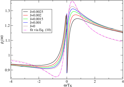
Figure 5: The Fano lineshape for $\rho_{c}(\omega)$ (in unit of $\rho_{0}$) for different antiferromagnetic RKKY couplings $J$ by NRG. The dashed line is a fit to the Fano lineshape form Eq. 10 for J=0. The other parameters are the same as in Fig. 1.

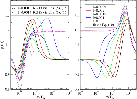
Figure 6: The Fano lineshape for $\rho_{c}(\omega)$ (in unit of $\rho_{0}$) on a logarithmic scale of $\omega/T_{k}$ for different antiferromagnetic RKKY couplings $J$ by NRG (solid lines) and perturbative RG via Eqs. 6 and 15 (dashed lines). The dot-dashed lines are fits to the Fano lineshape form via Eq. 10 for $J=0$. The dotted lines are the RG fits via Eqs. 5 and 15. The other parameters are the same as in Fig. 1.

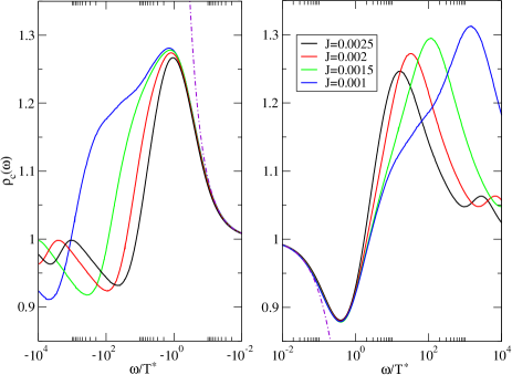
Figure 7: The Fano lineshape for $\rho_{c}(\omega)$ (in unit of $\rho_{0}$) on a logarithmic scale of $\omega/T^{*}$ for different antiferromagnetic RKKY couplings $J$ by NRG. The other parameters are the same as in Fig. 1. The dot-dash lines are power-law fits to the universal scaling function of $\omega/T^{*}$ via Eq. 20.

From the perturbative RG results, as $\omega\rightarrow T^{*}$, $\tilde{J}(\omega)$ diverges, leading to the vanishing LDOS. As $\omega$ decreases to $T^{*}$ from above, the factor $1-\frac{3\tilde{J}^{2}(\omega)}{16\tilde{T}_{k}^{2}}$ in Eq. LABEL:analyticReGd first becomes negative then it approaches $0$ as $\omega$ further approaches $0$. This explains the additional dip-peak structure seen for $|\omega|\rightarrow T^{*}$ in the NRG results. This qualitative feature can be captured by the perturbative RG approach. However, the magnitudes of the dip-peak features via perturbative RG are much smaller than those obtained from NRG. We believe the reasons for the deviation are two folds: First, the overall shape of $ReG_{d1}(\omega)$ predicted via RG is shifted towards the smaller $|\omega|$ region compared to the NRG results. This leads to a smaller value for $\omega_{0}>0$ (compared to that via NRG) where $ReG_{d1}(|\omega|<\omega_{0})$ changes its sign from positive (negative) to negative (positive) for $0<\omega<\omega_{0}$ ($-\omega_{0}<\omega<0$). This makes the magnitudes of these additional dips and peaks smaller as $\tilde{J}(\omega)$ diverges even further (see Eq. LABEL:analyticReGd). As $J$ is further increased, the deviations between RG and NRG become more transparent. This is expected as the perturbation theory becomes uncontrolled once the system moves away from the weak coupling regime. Nevertheless, the perturbative RG approach can still capture the qualitative features of $ReG_{d1}(\omega)$ for $T^{*}<|\omega|<T_{k}$ (see Fig. 2 and Fig. 3). Note that the perturbative RG approach via Eq. 6 (the Dyson’s equation) can fit the NRG result for $ReG_{d1}(\omega)$ better than that via Eq. 5 for $\omega\geq T_{k}$, as expected. Similar to the KT scaling behavior for $ImG_{d1}(\omega)$, the NRG results for $ReG_{d1}(\omega)$ also show a scaling behavior for $\omega\leq T^{*}$: $ReG_{d1}(\omega)\approx g_{0}^{\prime}g^{\prime}(\omega/T^{*})$ (see Fig. 4). Here, the scaling function $g^{\prime}(\omega/T^{*})$ is again completely universal in the case of particle-hole symmetry. Based on the Fermi liquid theory, the very low energy ($\omega\ll T^{*}$) crossover function for $ReG_{d1}(\omega)$ is linear in $\omega/T^{*}$ (see, for example Eq. 9):

$$\Gamma ReG_{d1}(\omega)\approx-a_{2}(\frac{\omega}{T^{*}}).$$ (19)

where we find $a_{2}\approx 1.5$ from the fit to the NRG result (see Fig. 4).

Finally, we discuss the behavior for the Fano lineshape for $\rho_{c}(\omega)$. As indicated in Eq. 16, the Fano lineshape for $\delta\rho_{c}(\omega)$ is effectively a linear combination of the asymmetric real part and symmetric imaginary part of the $G_{d1}(\omega)$. The parameter $q_{c}$ in Eq. 16 depends on the conduction electron reservoir. Following Ref. kroha and Ref. xiang , $q_{c}$ can be reasonably treated as a constant. We take a realistic value $q_{c}\approx 1.4$ here, corresponding to the $Co/Au$ system studied in Ref. xiang and Ref. wingreen . We find $\rho_{c}(\omega)$ is asymmetric with respect to $\omega=0$ with a larger magnitude for $\omega>0$ than that for $\omega<0$. As shown in Fig. 6 and Fig. 7, $\rho_{c}(\omega)$ shows a dips at $\omega\approx-T_{k}$ and $\omega\approx T^{*}$ as well as peaks at $\omega\approx T_{k}$ and $\omega\approx-T^{*}$. The peak (dip) at $\omega\approx\pm T_{k}$ correspond to the first stage Kondo effect; while the dip (peak) at $\omega\approx\pm T^{*}$ correspond to the second stage Kondo effect via RKKY coupling. We find a reasonably good agreement between the NRG results and the fit via the perturbative RG approach for $T_{k}\approx\omega<T^{*}$. (The fit via Eq. 6 is somewhat better than that via Eq. 5 as the former gives a better fit to the NRG result for $ReG_{d1}(\omega)$ The above dip-peak structure in the Fano lineshpe for $\rho_{c}(\omega)$ in the presence of RKKY coupling can be detected in the STM measurement of the conduction electron leads as the signature of the two-stage Kondo effect in side-coupled double quantum dot. Note that the $\omega/T^{*}$ scaling in the NRG results for $\rho_{c}(\omega)$ is observed (see Fig. 5, and Fig. 6), which comes naturally from the scaling behaviors for both real and imaginary parts of $G_{d1}(\omega)$ (see Eq. 3 and Fig. 7). In the low energy limit $\omega\ll T^{*}$ where the system approaches to the Fermi-liquid of local spin singlet, we have the following approximated power-law scaling behavior for $\delta\rho_{c}(\omega)$:

$$\frac{\delta\rho_{c}(\omega)}{\rho_{0}}\approx-[(1-q_{c}^{2})a_{1}(\frac{\omega}{T^{*}})^{2}+2a_{2}q_{c}\frac{\omega}{T^{*}}].$$ (20)

We would like to make one side remark here. For $\omega\ll T_{k}$, the single Lorentzian approximation Eq. 5 can very well describe $G_{d1}(\omega)$; however, for $\omega\leq T_{k}$, we expect a finite contribution to $G_{d1}(\omega)$ from interference between the Kondo resonance and the broadened impurity level at dot $1$. We find indeed a better agreement between the analytic fits and the NRG results for $G_{d1}(\omega)$ and $\rho_{c}(\omega)$ via perturbative RG approach based on the Dyson’s equation Eq. 6 than those from the single Lorentzian fit via Eq. 5.

V. Conclusions.

We have studied the Fano resonance in a side-coupled double-quantum-dot system in the Kondo regime in the presence of particle-hole symmetry. In the range where the energy of the dot $1$ is of the order of the broadening of its energy level, quantum interference between the Kondo effect and the broadened energy level of the dot $1$ gives rise to modification of the Green’s function on dot $1$. We apply the perturbative and numerical renormalization group approaches to describe the Fano lineshape in TDOS of the conduction electrons, which depend on both the real and imaginary parts of the Green’s function $G_{d1}(\omega)$ of the dot $1$. At $J=0$, $ImG_{d1}(\omega)$ shows the Kondo peak for $\omega\leq T_{k}$; while $ReG_{d1}(\omega)$ exhibits a peak (dip) for $\omega\approx T_{k}$ ($\omega\approx-T_{k}$). As a result of the Kondo effect, the Fano lineshape in TDOS of the conduction electron leads shows a peak (dip) around $\omega\approx T_{k}$ ($\omega\approx-T_{k}$). At a finite antiferromagnetic spin exchange coupling between the two dots, the two-stage Kondo effect leads to the suppression of the density of states on dot $1$ as well as an additional dip (peak) structure in the real part of $G_{d1}(\omega)$ at $\omega\approx\pm T^{*}$ from the NRG results. This leads to an additional dip (peak) around $\omega\approx T^{*}$ ($\omega\approx-T^{*}$) in the conduction electron LDOS. The spliting between dip and peak in LDOS at $\omega\approx\pm T^{*}$ becomes more pronounced as the RKKY coupling $J$ is increased. At finite values of $J$ and for $\omega<T^{*}$, the NRG results for $ReG_{d1}(\omega)$, $ImG_{d1}(\omega)$ and $\rho_{c}(\omega)$ all show distinct universal scaling behaviors in $\omega/T^{*}$. Analytically, we find the perturbative RG approach can qualitatively capture the above behaviors for $T^{*}\ll\omega\leq T_{k}$. In particular, compare to the simple Lorentzian approximation for $G_{d1}(\omega)$, we find a better fit to the NRG results for the Fano lineshape for $\rho_{c}(\omega)$ for $T^{*}\ll\omega\leq T_{k}$ by taking into account the interference between the Kondo resonance and the broadened impurity level on dot $1$ within the Dyson’s equation approach. To make contact of our results in the experiments, the asymmetrical double dip/peak structure and the scaling behaviors in the Fano lineshape predicted here in the spectral properties of the TDOS of the conduction electron leads can be dectcted by the transport through the STM tipskroha as an indication and direct consequence of the two-stage Kondo effect in our side-coupled double-quantum-dot system. Finally, we would like to make a remark on the Fano lineshape in TDOS of the leads in our system without particle-hole symmetry. In this case, we expect a smooth crossover (instead of the KT type transition) between the Kondo and local singlet phases due to the potential scattering terms generated in the presence of particle-hole asymmetry. Nevertheless, further investigations via NRG are needed to clarify this issue.

- (1) U. Fano, Phys. Rev. 124, 1866 (2961).
- (2) A.C. Hewson, The Kondo Problem to Heavy Fermions (Cambridge University Press, Cambridge, UK, 1997).
- (3) H.G. Luo, T. Xiang, Z.B. Su and L. Yu, Phys. Rev. Lett. 92, 256602 (2004); H.G. Luo, T. Xiang, Z.B. Su and L. Yu, Phys. Rev. Lett. 96, 019702 (2006).
- (4) O. Ujsaghy , J. Kroha, L. Szunyogh, A. Zawadowski, Phys. Rev. Lett. 85, 2557 (2000); Ch. Kolf, J. Kroha, M. Ternes, and W.-D. Schneider, Phys. Rev. Lett. 96, 019701 (2006).
- (5) A. Schiller and S. Hershfield, Phys. Rev. B 61, 9036 (2000).
- (6) M. Plihal and J. W. Gadzuk, Phys. Rev. B 63, 085404 (2001).
- (7) V. Madhaven, W. Chen, T. Jamneala, M.F. Crommie and N.S. Wingreen, Science 280, 567 (1998); Phys. Rev. B 64, 165412 (2001).
- (8) J. Li, W.D. Schneider, R. Berndt, and B. Delley, Phys. Rev. Lett. 80, 2893, (1998); N. Knorr, M.A. Schneider, L. Diekhoner, P. Wahi, and K. Kern, Phys. Rev. Lett. 88, 096804 (2002); M.A. Schneider, L. Vitali, N. Knorr, and K. Kern, Phys. Rev. B 65, 121406 (2002).
- (9) H.C. Manoharan, C.P. Lutz, and D.M. Eigler, Nature 403, 512 (2000).
- (10) W. Hofstetter, J. Koenig, and H. Schoeller, Phys. Rev. Lett. 87, 156803 (2001).
- (11) M. Sato et al., Phys. Rev. Lett. 95, 066801 (2005).
- (12) S. Sasaki, H. Tamura, T. Akazaki, and T. Fujisawa, arXiv:0912.1926.
- (13) W.-R. Lee, Jaeuk U. Kim, H.-S. Sim, Phys. Rev. B 77, 03305 (2008).
- (14) Tetsufumi Tanamoto, Yoshifumi Nishi, Shinobu Fujita, J. Phys.: Condens. Matter 21 (2009) 145501.
- (15) A.W. Rushforth et al., Phys. Rev. B 73, 081305 (R) (2006).
- (16) Chung-Hou Chung, Gergely Zarand and Peter Wölfle, Phys. Rev. B 77, 035120 (2008).
- (17) P.S. Cornaglia and D. R. Grempel, Phys. Rev. B 71, 075305 (2005).