Simultaneous denoising and enhancement of signals by a fractal conservation law

Abstract

In this paper, a new filtering method is presented for simultaneous noise reduction and enhancement of signals using a fractal scalar conservation law which is simply the forward heat equation modified by a fractional anti-diffusive term of lower order. This kind of equation has been first introduced by physicists to describe morphodynamics of sand dunes. To evaluate the performance of this new filter, we perform a number of numerical tests on various signals. Numerical simulations are based on finite difference schemes or Fast Fourier Transform. We used two well-known measuring metrics in signal processing for the comparison. The results indicate that the proposed method outperforms the well-known Savitzky-Golay filter in signal denoising. Interesting multi-scale properties w.r.t. signal frequencies are exhibited allowing to control both denoising and contrast enhancement.

Keywords: fractal operator, fractional calculus, Fourier transform, PDEs filters, denoising, enhancement, fast Fourier transform (FFT), finite difference scheme, Savitzky-Golay filter.

AMS Subject Classifications: 35R11; 60G35; 26A33.

1 Introduction

Filtering is a process that removes some unwanted component from a signal. It is a very important task in signal processing, data analysis and communication systems. Many techniques have been proposed for this purpose. For instance, we can use simple averaging filters such as a Gaussian filter. It is well-known that this filter can be realized by solving the heat equation. Other more general partial differential equations (PDE) have been used, with non-linear anisotropic diffusion [6, 22], non-linear fractional diffusion [4, 15] or fractional time-derivative [7]. It has been proved that PDEs are suitable in signal denoising [20]. The denoising applications have to take into account two points. First, we want to obtain a clean and readily observable signal (improving signal-to-noise ratio SNR) and secondly, preserve the original shape characteristics (maxima, minima…) of the signal. This task is complex because it is very important that the denoising has no blurring effect on the images and does not change the location of image edges, [5]. For some applications, it is interesting to amplify some features of the signal such as relative maxima or minima in order to enhance its contrast. Usually, these features are flattened by the denoising methods based on averaging techniques. Among the denoising methods which preserve characteristics of the initial signal is the Savitzky-Golay filter, with which we will compare our new method.

A basic and crude idea to enhance the contrast could be to solve the backward heat equation for a few time steps. Of course, this is an ill-posed PDE and we do not advocate this unsafe method but it illustrates the fact that enhancement and denoising are antagonistic operations. Our method is based on a linear PDE, with two antagonistic terms : a usual diffusion and a nonlocal fractional anti-diffusive term of lower order. The diffusion is used to reduce the noise whereas the nonlocal anti-diffusion is used to enhance the contrast. Let us emphasize that we perform at the same time noise reduction and contrast enhancement. Our method is based on the Cauchy problem of the following PDE :

$$\begin{cases}\partial_{t}u(t,x)-a\,\partial_{xx}^{2}u(t,x)+b\,\mathcal{I}_{\lambda}[u(t,.)](x)=0&t\in(0,T),x\in\mathbb{R},\\ u(0,x)=u_{0}(x)&x\in\mathbb{R},\end{cases}$$ (1)

where $T$ is any given positive time, $u_{0}\in L^{2}(\mathbb{R})$, $a,\,b$ are positive constants and $\mathcal{I}_{\lambda}$ is a fractional operator defined as follows via the Fourier transform: for any Schwartz function $\varphi\in\mathcal{S}(\mathbb{R})$

$$\mathcal{I}_{\lambda}[\varphi](x):=-\,\mathcal{F}^{-1}(|.|^{\lambda}\mathcal{F}(\varphi))(x)\,$$ (2)

where $0<\lambda<2$ and $\mathcal{F}$ denote the Fourier transform defined by: for all $\xi\in\mathbb{R}$

$$\mathcal{F}f(\xi):=\int_{\mathbb{R}}e^{-2i\pi x\xi}f(x)dx.$$

Let us note that for $\lambda\in]1,2[$, we have an explicit nonlocal formula (see proposition 5)

$$\mathcal{I}_{\lambda}[\varphi](x)=\alpha_{\lambda}\int_{\mathbb{R}}\frac{\varphi^{{}^{\prime\prime}}(x-\xi)}{|\xi|^{\lambda-1}}d\xi$$ (3)

where $\alpha_{\lambda}$ is a suitable constant.
Alternatively, we can also give a slightly different definition, inspired by fractional calculus (see remark below) :

$$\mathcal{I}_{\lambda}[\varphi](x)=\alpha_{\lambda}\int_{0}^{+\infty}\frac{\varphi^{{}^{\prime\prime}}(x-\xi)}{|\xi|^{\lambda-1}}d\xi.$$ (4)

Remark 1.

For causal signals (i.e $\varphi(x)=0$ for $x<0$) we have

$$\frac{1}{\Gamma(2-\lambda)}\int_{0}^{+\infty}\frac{\varphi^{{}^{\prime\prime}}(x-\xi)}{|\xi|^{\lambda-1}}d\xi=\frac{d^{\lambda-2}}{dx^{\lambda-2}}\varphi^{\prime\prime}=\frac{d^{\lambda}}{dx^{\lambda}}\varphi$$ (5)

which is exactly the Riemann Liouville definition of the fractional derivative [23].

Remark 2.

Our model is closely related to a nonlocal conservation law first introduced to describe the morphodynamics of sand dunes and ripples sheared by a fluid flow. Namely, Fowler ([12, 13, 14]) introduced the following equation

$$\partial_{t}u(t,x)+\partial_{x}\left(\frac{u^{2}}{2}\right)(t,x)+\mathcal{I}[u(t,.)](x)-\partial_{xx}^{2}u(t,x)=0,$$ (6)

where $u=u(t,x)$ represents the dune height and $\mathcal{I}$ is a nonlocal operator defined as follows: for any Schwartz function $\varphi\in\mathcal{S}(\mathbb{R})$ and any $x\in\mathbb{R}$,

$$\mathcal{I}[\varphi](x):=\int_{0}^{+\infty}|\zeta|^{-\frac{1}{3}}\varphi^{\prime\prime}(x-\zeta)d\zeta.$$ (7)

Equation (6) is valid for a river flow over a erodible bottom $u(t,x)$ with slow variation. The nonlocal term appears after a subtle modeling of the basal shear stress. See [1, 2] for theoretical results on this equation.
This nonlocal term appears also in the work of Kouakou & Lagree [17, 18]. The operator $\mathcal{I}[u]$ is a weighted mean of second derivatives of $u$ with the bad sign and has therefore an anti-diffusive effect and create instabilities which are controlled by the diffusive operator $-\partial_{xx}^{2}$. We find again this phenomenon for the equation (1).

The solution of the linear PDE (1) is obtained by convolution with the kernel $K$ of $\mathcal{I}_{\lambda}-\partial_{xx}^{2}$. Thereafter, this kernel will be our filter for denoising and enhancement of signals. The analysis of this kernel shows that the low frequencies are preserved, the medium frequencies are amplified and the high frequencies are eliminated. It is clear that this kernel depends on the parameters $a,b,\lambda$ and that the choice of these coefficients will determine the quality of the noise reduction and of the enhancement. In this paper, we discuss the choice of these parameters.
To evaluate the performance of our filter, we discretize the PDE by two methods : the fast Fourier transform and the finite difference method. Numerical studies of nonlocal equations are rather scarce: among them, we mention [11] which proves the convergence of a finite volume method to approximate the solutions of a fractal scalar conservation law, that is to say a conservation law regularized by a diffusive fractional power of the Laplace operator and [3] which analyzes the stability of finite difference schemes for the solution of (6). In these works, the discretization of the fractal operator is performed via an integral formula for $\mathcal{I}_{\lambda}$ similar to the ones appearing in [1, 9]. Our method is then compared with the Savitzky-Golay filter. Results show that the PDE (1) is relevant and effective for denoising with preservation or enhancement of features of the signal.

The remaining of this paper is organized as follows: in the next section, we explicit the solution of problem (1) and we give some properties of the kernel. In section 3, we present explicit numerical schemes which approximate the fractal conservation law (1) and we give some numerical simulations. In this section, we also briefly present the Savitzky-Golay filter and compare it with our filter. Other numerical simulations based on the FFT are given in section 4. We also discuss the choice of parameters $a,b,\lambda$ and we highlight both the ability of denoising and contrast enhancement of our model. Section 5 is devoted to the performance evaluation and metrics. Section 6 gives conclusions about this study.

2 Theoretical study of the PDEs

In this section, we verify that (1) is well-posed and in subsection 2.2 we analyze the properties of the kernel $K$ of $\mathcal{I}_{\lambda}-\partial_{xx}^{2}$, for $0<\lambda<2$.

2.1 Well-posedness of the problem

Using the Fourier transform, we see that any solution to (1) satisfies the formula (8).

Proposition 1.

Let $T>0$ and $u_{0}\in L^{2}(\mathbb{R})$. The function $u\in L^{\infty}((0,T);L^{2}(\mathbb{R}))$ is a solution of (1) if for any $t\in\left(0,T\right)$:

$$u(t,x)=K(t,\cdot)\ast u_{0}(x)$$ (8)

where $K(t,x)=\mathcal{F}^{-1}\left(e^{-t\psi(\cdot)}\right)(x)$ with $\psi(\xi):=4\pi^{2}a\xi^{2}-b\,|\xi|^{\lambda}$ is the kernel of the operator $\mathcal{I}_{\lambda}-\partial^{2}_{xx}$.

Proposition 2.

Let $T>0$, $u_{0}\in L^{2}(\mathbb{R})$. Then, the function

$$u:t\in(0,T]\rightarrow K(t,\cdot)\ast u_{0}$$

is well-defined and belongs to $C([0,T];L^{2}(\mathbb{R}))$: $u$ is extended at $t=0$ by the value $u(0,.)=u_{0}$.

Proof.

We have

$$K(t,x)=\int_{\mathbb{R}}e^{2i\pi x\xi}\,h(\xi)\,d\xi,$$

where $h(\xi)=e^{-t\psi(\xi)}$. For $0<\lambda<2$, it is easy to verify that $h$ belongs to $W^{2,1}(\mathbb{R})$ where $W^{2,1}(\mathbb{R}):=\left\{v\in L^{1}(\mathbb{R});\frac{\partial v}{\partial x},\frac{\partial^{2}v}{\partial x^{2}}\in L^{1}(\mathbb{R})\right\}$ therefore we have that $K(t,.)\in L^{1}(\mathbb{R})$. Hence, $\forall t>0$, $K(t,\cdot)*u_{0}$ is in $L^{2}(\mathbb{R})$.

Let us prove the strong continuity ie

$$\lim_{t\to 0}K\left(t,.\right)*u_{0}=u_{0}\hskip 5.69046ptin\hskip 5.69046ptL^{2}\left(\mathbb{R}\right).$$

By Plancherel’s formula,

$$||K(t,\cdot)\ast u_{0}-u_{0}||^{2}_{L^{2}(\mathbb{R})}=||\mathcal{F}(K(t,\cdot)\ast u_{0})-\mathcal{F}u_{0}||^{2}_{L^{2}(\mathbb{R})}\\ =||e^{-t\psi}\mathcal{F}u_{0}-\mathcal{F}u_{0}||^{2}_{L^{2}(\mathbb{R})}=\int_{\mathbb{R}}|e^{-t\psi}-1|^{2}\,|\mathcal{F}u_{0}|^{2}.$$ (9)

Since the function $|e^{-t\psi}-1|^{2}\,|\mathcal{F}u_{0}|^{2}$ converges pointwise to $0$ on $\mathbb{R}$, as $t\rightarrow 0$ and as $\min\psi$ is finite then, by the dominated convergence theorem, the last term of (9) tends to $0$ as $t\rightarrow 0$.

∎

Remark 3 (Regularity of the solution).

It is easy to see that $u\in C^{\infty}((0,T]\times\mathbb{R})$ because $K$ is smooth. The smoothness of $K$ is an immediate consequence of the theorem of derivation under the integral sign applied to the definition of $K$ by Fourier transform. To obtain the regularity at $t=0$, we have to suppose that the initial condition $u_{0}$ is in $C^{\infty}(\mathbb{R})$ and satisfies for all $k\in\mathbb{N}$, $u_{0}^{(k)}\in L^{2}(\mathbb{R})$. The proof is similar with replacing $u_{0}$ by $u_{0}^{(k)}$.

Remark 4.

From formula (8), it is straightforward that

$$\int_{\mathbb{R}}u(t,x)\,dx=\mathcal{F}\left(K(t,\cdot)\right)(0)\cdot\int_{\mathbb{R}}u_{0}(x)\,dx=\int_{\mathbb{R}}u_{0}(x)\,dx.$$ (10)

This is a “mass conservation” property.

2.2 Study of the kernel

In this subsection, we give some properties on the kernel $K$ of $\mathcal{I}_{\lambda}-\partial_{xx}^{2}$.

Proposition 3.

The kernel $K$ has a non-zero negative part.

Proof.

Let us assume that $K$ is nonnegative, then

$$|e^{-t\psi(\xi)}| \leq ||\mathcal{F}^{-1}(e^{-t\psi})||_{L^{1}(\mathbb{R})}=\int_{\mathbb{R}}|K(t,.)|$$

$$= \int_{\mathbb{R}}K(t,.)=\mathcal{F}(K(t,.))(0)=e^{-t\psi(0)}=1$$

for all $\xi\in\mathbb{R}$. But we have for $0<|\xi|<\left(\frac{b}{4\pi^{2}a}\right)^{\frac{1}{2-\lambda}}$, $|e^{-t\psi(\xi)}|=e^{-t(4\pi^{2}a\xi^{2}-b|\xi|^{\lambda})}>1$ , this yields a contradiction. ∎

The main consequence of the non-positivity of $K$ is the failure of the maximum principle for the equation (1) [1]. Thereby, $u(x,t)$ is not forced to remain in the interval $[\min(u_{0}),\max(u_{0})]$. The signal can then be amplified when it is necessary.
Using the proof of the previous proposition, we can deduce that the enhancement of the frequencies will be feasible only for the low/medium frequencies. Of course, this amplification will depend on the choice of the parameters $a,b,\lambda$ and of the time $t$.

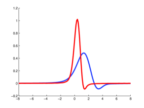
(a) The kernel of $\mathcal{I}_{\lambda}$ for $t=0.1$ (red) and $t=0.5$ s (blue)

(b) Behaviour of $\psi$

Figure 1: $a=0.5,b=2$ and $\lambda=1.5$

We expose in figure 1 the evolution of $K(t,.)$ for different times and the behaviour of $\psi$ for $a=0.5,b=2,\lambda=1.5$.

3 Finite difference schemes

In this section, we present a finite difference numerical scheme to directly approximate the solution to (1) for any $\lambda\in]0,2[$.

3.1 Integral representation of $\mathcal{I}_{\lambda}$

To approximate the nonlocal term, it is useful to give an integral formula for $\mathcal{I}_{\lambda}$:

Proposition 4 ([10, 16]).

If $\lambda\in]0,2[$, we have for all $\varphi\in\mathcal{S}(\mathbb{R})$, all $x\in\mathbb{R}$ and all $r>0$,

$$\mathcal{I}_{\lambda}[\varphi](x)=C_{\lambda}\left(\int_{-r}^{r}\frac{\varphi(x+z)-\varphi(x)-\varphi^{{}^{\prime}}(x)z}{|z|^{1+\lambda}}\,dz+\int_{\mathbb{R}\setminus(-r,r)}\frac{\varphi(x+z)-\varphi(x)}{|z|^{1+\lambda}}\,dz\right)$$

where $C_{\lambda}=\frac{\lambda\Gamma(\frac{1+\lambda}{2})}{2\pi^{{\frac{1}{2}+\lambda}}\Gamma(1-\frac{\lambda}{2})}$ and $\Gamma$ denote the Euler function.

• If $\lambda\in]0,1[$ then

  $$\mathcal{I}_{\lambda}[\varphi](x)=C_{\lambda}\int_{\mathbb{R}}\frac{\varphi(x+z)-\varphi(x)}{|z|^{1+\lambda}}\,dz.$$ (11)

• If $\lambda\in]1,2[$ then

  $$\mathcal{I}_{\lambda}[\varphi](x)=C_{\lambda}\int_{\mathbb{R}}\frac{\varphi(x+z)-\varphi(x)-\varphi^{{}^{\prime}}(x)z}{|z|^{1+\lambda}}\,dz.$$ (12)

From this proposition, we deduce the following useful result :

Proposition 5.

For all $\varphi\in\mathcal{S}(\mathbb{R})$ and all $x\in\mathbb{R}$ we have for $\lambda\in]1,2[$

$$\mathcal{I}_{\lambda}[\varphi](x)=\alpha_{\lambda}\int_{\mathbb{R}}\frac{\varphi^{{}^{\prime\prime}}(x+z)}{|z|^{\lambda-1}}\,dz=\alpha_{\lambda}\int_{\mathbb{R}}\frac{\varphi^{{}^{\prime\prime}}(x-z)}{|z|^{\lambda-1}}\,dz$$ (13)

where $\alpha_{\lambda}=\frac{C_{\lambda}}{\lambda(\lambda-1)}$.

Proof.

The regularity of $\varphi$ ensures the validity of the following computations . Since

$$\varphi(x+z)-\varphi(x)-\varphi^{{}^{\prime}}(x)z = \int_{0}^{z}\left(\varphi^{{}^{\prime}}(x+y)-\varphi^{{}^{\prime}}(x)\right)\,dy$$

$$= \int_{0}^{1}\left(\varphi^{{}^{\prime}}(x+tz)-\varphi^{{}^{\prime}}(x)\right)\,z\,dt,$$

the last equality arises from the change of variable $y=tz$. Then, using Fubini’s Theorem, we have

$$\mathcal{I}_{\lambda}(x) = C_{\lambda}\int_{\mathbb{R}}\int_{0}^{1}(\varphi^{{}^{\prime}}(x+tz)-\varphi^{{}^{\prime}}(x))\,\frac{z}{|z|^{1+\lambda}}\,dt\,dz$$

$$= \int_{0}^{1}\left(\int_{\mathbb{R}}(\varphi^{{}^{\prime}}(x+tz)-\varphi^{{}^{\prime}}(x))\,\frac{z}{|z|^{1+\lambda}}\,dz\right)dt$$

$$\underbrace{=}_{y=tz} C_{\lambda}\int_{0}^{1}\left(\int_{\mathbb{R}}(\varphi^{{}^{\prime}}(x+y)-\varphi^{{}^{\prime}}(x))\frac{y}{|y|^{1+\lambda}}\,dy\right)t^{\lambda-1}\,dt$$

$$= C_{\lambda}\int_{0}^{1}t^{\lambda-1}\,dt\int_{\mathbb{R}}(\varphi^{{}^{\prime}}(x+y)-\varphi^{{}^{\prime}}(x))\frac{y}{|y|^{1+\lambda}}\,dy$$

$$= \frac{C_{\lambda}}{\lambda}\int_{\mathbb{R}}\left(\int_{0}^{1}\varphi^{{}^{\prime\prime}}(x+sy)y\,ds\right)\frac{y}{|y|^{1+\lambda}}\,dy$$

$$\underbrace{=}_{z=sy} \frac{C_{\lambda}}{\lambda}\int_{\mathbb{R}}\frac{\varphi^{{}^{\prime\prime}}(x+z)}{|z|^{\lambda-1}}\,dz\int_{0}^{1}s^{\lambda-2}\,ds$$

$$= \frac{C_{\lambda}}{\lambda(\lambda-1)}\int_{\mathbb{R}}\frac{\varphi^{{}^{\prime\prime}}(x+z)}{|z|^{\lambda-1}}\,dz.$$

∎

3.2 The numerical scheme

The spatial discretization is given by a set of points ${x_{i};i=1,...,N}$ and the discretization in time is represented by a sequence of times $t^{0}=0<...<t^{n}<...<T$. For the sake of simplicity we will assume constant step size $\delta x$ and $\delta t$ in space and time, respectively. The discrete solution at a point will be represented by $u^{n}_{i}\approx u(t^{n},x_{i})$. In this section, we will present the behaviour of explicit numerical scheme which directly approximate the solution to (1).

We discretize all terms of the equation using an explicit method. We consider for any $n,j\in\mathbb{N}$

$$\frac{u_{j}^{n+1}-u_{j}^{n}}{\delta t}-a\,\frac{u_{j+1}^{n}-2u_{j}^{n}+u_{j-1}^{n}}{\delta x^{2}}+b\,\mathcal{I}_{\delta x}[u^{n}]_{j}=0$$ (14)

where $\mathcal{I}_{\delta x}$ is a discretization of the nonlocal term $\mathcal{I}_{\lambda}$. This scheme is explicit because the values of the solution at time $t^{n+1}$ are obtained directly from the (known) values at time $t^{n}$. For the Laplacian term, we use a standard centered finite difference approximation of second order. To discretize the fractal operator $\mathcal{I}_{\lambda}$, we consider the formulation (4), which for $\lambda\in]1,2[$ is a causal variant of (13). Next, we use a basic quadrature rule to approximate the integral and we use a finite difference approximation of the derivative:

$$\mathcal{I}_{\delta x}[v]_{j}=\delta x^{-\lambda}\,\sum^{+\infty}_{l=1}l^{1-\lambda}(v_{j-l+1}-2v_{j-l}+v_{j-l-1});$$ (15)

Note that we have absorbed the constant $\alpha_{\lambda}$ in $b$.

Remark 5.

The practical implementation of the schemes requires to make truncations. The main truncation concerns the integral operator for the nonlocal term $\mathcal{I}_{\lambda}$. We replace $\int_{0}^{+\infty}$ with $\int_{0}^{L}$ and the finite difference approximation becomes:

$$\mathcal{I}_{\delta x}[v]_{j}=\delta x^{-\lambda}\,\sum^{A}_{l=1}l^{1-\lambda}(v_{j-l+1}-2v_{j-l}+v_{j-l-1});$$ (16)

with $L=A\,\delta x$. Usually, we consider that functions are either compactly supported or constant near $-\infty$ and $+\infty$, so it is legitimate to consider a finite sum for the discretization of $\mathcal{I}_{\lambda}$. However the truncation parameter $A$ has to be chosen judiciously. Indeed, when $0<\lambda<1$ , the term $l^{1-\lambda}$ in the discretization (16) is bigger and bigger for increasing $l$, hence $A$ ought to be big enough. In contrast, whenever $1<\lambda<2$, $l^{1-\lambda}$ is negligible for large values and is important only for small values of $l$. Thus in this case, it is judicious to take $A$ small enough. We see again here that the non local effect is all the more important than $\lambda$ is small. These memory effects strongly depending on $\lambda$ have been reported in [8]. To take this behaviour into account, we set the truncation parameter $A:=\max(100,\frac{10}{\lambda})$. Of course $100$ is an arbitrary limit to avoid rounding effects for small $\lambda$.

Since the equation is implemented using an explicit method, this imposes a CFL condition on the time and space steps which ensures the numerical stability that is to say that the difference between the approximate solution and the exact solution remains bounded when $n\rightarrow+\infty$ for $\delta x,\delta t$ given. The stability analysis of the nonlocal scheme (14) is done in [3]. This requires a careful study, owing to the anti-diffusive behaviour of the nonlocal term. Indeed, the analysis of the PDE (1) shows that for the continuous problem, low to medium frequencies are amplified by the nonlocal term, [3]. We come back to this in section 4. Therefore, the standard Von Neumann definition of stability must be slightly modified. Denoting $\theta=k\,\delta x\in(0,2\pi)$ and $u^{n}_{j}=\exp{(ij\theta)}$, instead of imposing that the amplification factor $G(\theta)=\frac{u^{n+1}_{j}}{u^{n}_{j}}$ must fulfill $|G(\theta)|<1$ for any frequency $\theta$, we only impose $|G(\theta)|<1$ for $\theta$ above a given threshold. We obtain the two following conditions on the time and space steps:

$$(1-2^{1-\lambda})\,\frac{b}{\delta x^{\lambda}}<\frac{2a}{\delta x^{2}},$$ (17)

$$\frac{2a\,\delta t}{\delta x^{2}}+(2-2^{1-\lambda})\,\frac{b\,\delta t}{\delta x^{\lambda}}<1.$$ (18)

The first stability condition (17) forces the mesh-size $\delta x$ to be small enough in order that the diffusion term should dominate the nonlocal anti-diffusive term for high frequencies, whereas the second stability condition (18) looks like an usual CFL condition for explicit schemes and forces the time-step to be small enough. For more details, we refer the reader to [3].

3.3 Numerical results

In the following numerical tests, we have to take care to choice $\delta t$ and $\delta x$ accuratly following the conditions (17) and (18). Thus, the time and space steps depend on the choice of $a,\,b$ and $\lambda$. We begin by consider an electrocardiogram (ECG) signal. Figure 2 illustrates a comparison between the PDE (1) implemented using a finite difference method (FDM) and the Savitzky-Golay smoothing filter.
The Savitzky-Golay smoothing filter also called digital smoothing polynomial filter or least-squares smoothing filter was first described in 1964 by Abraham Savitzky and Marcel J. E. Golay. [24]. Essentially, the Savitzky-Golay method performs a local polynomial regression on a series of values that is to say it replaces each value of the series with a new value which is obtained from a polynomial fit to neighboring points. The algorithm is based on the following equation

$$u_{j}=\left[a_{0}v_{j}+\sum_{i=1}^{\frac{n+1}{2}}a_{i}(v_{j-i}+v_{j+i})\right]$$

where $n$ is the number of data points, $a_{i}$ are (positive) constants, $v$ is the noisy signal and $u$ defines the filtered signal. The main advantage of this approach is the preservation of features of the signal such as relative maxima, minima and width. Indeed, usually these characteristics are ’flattened’ by classical averaging techniques such as moving averages. Figure 2 shows three plots: The noisy ECG signal, the smoothed signal (red) using the PDE filter (1) superimposed with the noiseless signal (blue) and the smoothed signal (red) using the Savitzky-Golay filter superimposed with the noiseless signal (blue). As we can remark, for these parameters, the low/medium frequencies are not amplified but the relative maxima and minima are preserved. The denoising seems correct and the filtering with our numerical scheme and with Savitzky-Golay seems similar, see better. We evaluate our approach and we compare it with Savitzky-Golay in section 5.

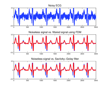
Figure 2: Top: a noisy electrocardiogram $u$; Middle: in red the noiseless signal, in blue the filtered signal with finite difference scheme (14) with $a=4,b=0.5,\lambda=1.7,\delta x=1$ and $\delta t=0.1$; Bottom : Noiseless signal (blue) vs. filtered signal using Savitzky-Golay filter.

Figure 3 illustrates two filtered signals of different types. We start from the simplest possible example of nonlocal filter denoising applied to a signal $u(x)$ consisting of a piecewise constant step function $v(x)=-1$ for $0<x<1$ and $v(x)=1$ for $1<x<2$ corrupted by additive Gaussian white noise $n(x)$ with standard deviation $\sigma=0.4$:

$$u(x)=v(x)+n(x).$$ (19)

The result of the denoising is illustrated in figure 3(a). As we can notice, the noise is very well eliminated and we find again our original signal, the shape of the signal has been preserved. The result is better than filtering Savitzky-Golay. Moreover, unlike Discrete Fourier Transform where the contrast is low in the neighbourhood of the discontinuity (see figure 5(a)), the dicontinuity/shock is conserved. Therefore, the finite difference method is more suitable for this kind of signal. Figure 3(b) shows another example of good denoising.

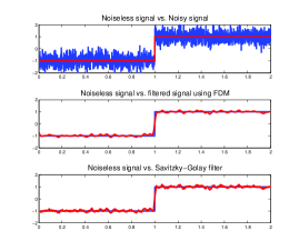
(a) $a=3.5,\,b=0.2,\,\lambda=0.1,\delta t=10^{-6}$ and     $\delta x=0.001$.

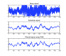
(b) $a=3.5,\,b=0.3,\,\lambda=1.1,\delta t=0.1$ and $\delta x=1$.

Figure 3: (a) Top: Noisy signal (blue) vs. noiseless signal (red); Middle: Noiseless signal (blue) vs. filtered signal using FDM (red); Bottom: Noiseless signal (blue) vs. filtered signal using Savitzky-Golay filter (red). (b) Top: Noisy signal; Middle: Noiseless signal ; Bottom: filtered signal using FDM .

4 Numerical results using Discrete Fourier Transform

In this section, we first discuss the choice of parameters $a,b,\lambda$ and next, we give some numerical results based on fast Fourier transform (FFT) which is an efficient algorithm to compute the discrete Fourier transform.

4.1 Choice of parameters

We fix $T=1$. So, we can rewrite the kernel in Fourier variable as follows:

$$K_{a,b}^{\lambda}(\xi)=e^{-\psi(\xi)}$$

where $\psi(\xi)=4\pi^{2}a\xi^{2}-b|\xi|^{\lambda}$.

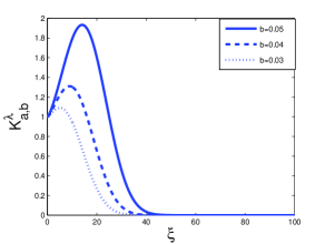
(a) $4\pi^{2}a=0.01$ and $\lambda=1.5$

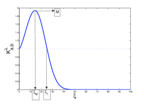
(b) $4\pi^{2}a=0.01$, $b=0.05$ and $\lambda=1.5$

Figure 4: Evolution of the spatial Fourier transform of the kernel $K$ for different parameters.

We draw in figure 4 the behaviour of the kernel $K_{a,b}^{\lambda}$ for $a,\lambda$ fixed and for different values of $b$. As $K_{a,b}^{\lambda}$ reaches it maximum at $\xi_{M}:=\left(\frac{\lambda b}{8\pi^{2}a}\right)^{\frac{1}{2-\lambda}}$ and $K_{a,b}^{\lambda}(\xi_{M})=e^{4\pi^{2}a(\frac{\lambda b}{8\pi^{2}a})^{\frac{2}{2-\lambda}}(\frac{2}{\lambda}-1)}$, we deduce that $K_{a,b}^{\lambda}(\xi_{M})>1$ if and only if $0<\lambda<2$. Therefore, whatever the choice of $\lambda\in]0,2[$ , we always have an amplification of medium frequencies. Of course, the magnitude of amplification depends on $a,b,\lambda$. Another natural frequency is $\xi_{1}=\left(\frac{b}{4\pi^{2}a}\right)^{\frac{1}{2-\lambda}}$ which represents the neutral frequency and satisfies $K^{\lambda}_{a,b}(\xi_{1})=1$ and $K^{\lambda}_{a,b}(\xi_{1})<1$ for $\xi>\xi_{1}$. Therefore $\xi_{1}$ is the threshold above which dampening will occur.

Now, we wish to control both the denoising and contrast enhancement. For that, we follow a simple strategy:

1. In a first step, we wish to control the frequency range to amplify. This one can be controlled by the following ratio: $\frac{\xi_{1}}{\xi_{M}}=(\frac{2}{\lambda})^{1/2-\lambda}$. Indeed, this ratio is decreasing w.r.t. parameter $\lambda$ and shrinks from $+\infty$ to $\sqrt{e}$ when $\lambda$ varies from $0$ to $2$. Hence, to choose a given amplified frequency range, it is enough to fix parameter $\lambda$ and the ratio $\frac{b}{a}$ (which in turn determines $\xi_{1}=\left(\frac{b}{4\pi^{2}a}\right)^{\frac{1}{2-\lambda}}$).

2. In this step, we want to monitor the denoising, which will start for frequencies above the neutral one $\xi_{1}$. One can easily check the following equality:

   $$\psi(\alpha\xi_{1})=4\pi^{2}a\,\xi_{1}^{2}(\alpha^{2}-\alpha^{\lambda})$$

   where $\alpha$ is a any positive constant. Therefore, the greater $a$ is, the smaller $K^{\lambda}_{a,b}(\alpha\xi_{1})$ will be, which means that the dampening rate will increase. Hence parameter $a$ monitors the denoising intensity, this is coherent because it controls the Laplacian term.

3. To finish with, we wish to monitor the value $M:=K^{\lambda}_{a,b}(\xi_{M})$ in order to control the contrast enhancement. Indeed, the higher $M$ is, the better the constrast will be amplified. Parameters $\lambda$ and $\frac{b}{a}$ being fixed by item 1 it is enough to adjust both parameters $b$ and $a$ while keeping the ratio $\frac{b}{a}$ within some bounds in order to preserve the amplified frequency range. The expression of $M$ shows that to have a good amplification of medium frequencies, it is necessary to increase $b$ as well as $a$. This is quite natural since the coefficient $b$ controls the anti-diffusive term and has an opposite behaviour to the Laplacian term which tends to flatten the signal. In our method, contrast and denoising are no more antagonistic. We come back on the tuning of parameter $b$ in section 5.

4.2 Denoising

In this subsection, we are only going to highlight the ability of noise reduction of our nonlocal equation (1).
To begin with, we consider an ECG signal to illustrate the denoising using the FFT to solve the fractal equation (1). The result is given in the figure 5(b).

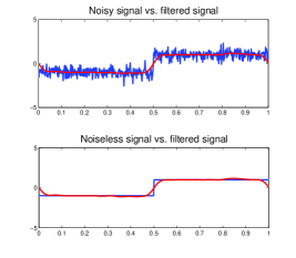
(a) $4\pi^{2}a=0.01,b=0.03$ and $\lambda=0.5$

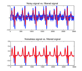
(b) $4\pi^{2}a=0.0051,b=0.015$ and $\lambda=1.7$

Figure 5: Top: Noisy signal (blue) vs. filtered signal (red). Bottom: noiseless signal (blue) vs. filtered signal (red).

For this choice of parameters, we note that the denoising is suitable and that the relative maxima are preserved. However, the relative minima are not completely preserved, in fig. 5(b) bottom. At last, Figure 10(a) describes the denoising of a sinusoidal signal. We can see the performance of the denoising of nonlocal approach discretized with FFT, which works very well for this type of periodic signal.

4.3 Denoising & Enhancement of signals

In this part, we are going to highlight both the ability of noise reduction and contrast enhancement. Of course, to emphasize the amplification, we take into account the remarks done in subsection 4.1.

We start from a simple example of simulatenous denoising and enhancement applied to a strongly attenuated sinusoidal signal highly corrupted by a random noise. In figure 6 middle, we plot the original noiseless signal, the same signal amplified $\times 50$ and the filtered signal, performed with our non local FFT method. As we can notice in figure 6, the noise is eliminated and the contrast is well amplified.

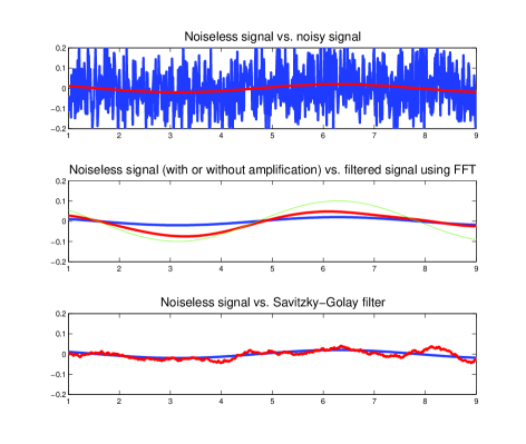
Figure 6: Top: Noisy signal (blue) vs. noiseless signal $v(x)=0.02\cos(x)$ (red); Middle: Noiseless signal (blue) vs. filtered signal (red) using FFT with $4\pi^{2}a=0.2,b=1.25,\lambda=0.5$ superimposed with amplified noiseless signal $cos(x)$ (green); Bottom: Noiseless signal (blue) vs. filtered signal (red) using Savitzky-Golay method.

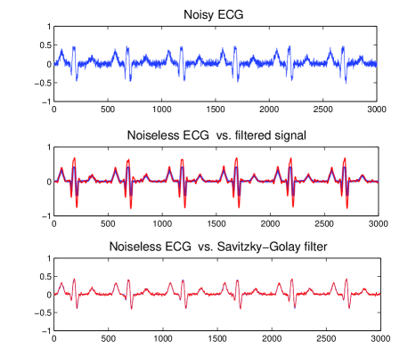
Figure 7: Top: a noisy electrocardiogram $u(x)$; Middle: the noiseless signal $v(x)$ (blue) and denoising & enhancement of the ECG signal (red) using the FFT on the fractal equation (1) with $4\pi^{2}a=0.005,b=0.0225$ and $\lambda=1.7$. Bottom: filtering using Savitzky-Golay method.

Figure 7 illustrates the smoothing of an electrocardiogram signal by filtering the noise with Savitzky-Golay filter (third plot) and by denoising and enhancement with the fractal scalar conservation law (1) (second plot). In the second case, we can see that the relative maxima and minima are amplified. Of course, we can obtain even greater amplification of low/medium frequencies by suitably tuning the parameters but, in these conditions, we will obtain sizeable variations between each peak. Thus, when we wish to amplify the low frequencies, we have to be careful that we do not alter too much the shape of the noiseless signal.

To rate the performance of denoising and enhancement of our filter, we consider signals with different SNR, which corresponds to the power ratio between a signal and the background noise.

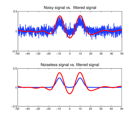
Figure 8: First plot (top) represents a noisy signal $u(x)$ (blue). Second plot (bottom) illustrates the noiseless signal $v(x)$ (blue) and denoising & enhancement of the signal (red) using the FFT on the fractal equation (1) with $4\pi^{2}a=0.1,b=0.3$ and $\lambda=1.5$.

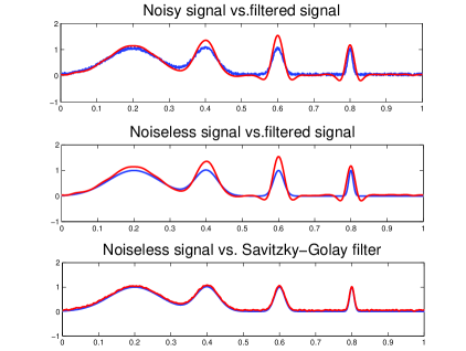
Figure 9: Choice of parameters: $4\pi^{2}a=0.01,b=0.05$ and $\lambda=1.5$. The red line depicts the filtered signal.

In figure 8, we took a small SNR. We can observe that shapes are amplified and that noise has been reduced significantly. But, we can also remark the undershoots just before and behind the shapes. This phenomenon has been highlighted in [1] in the setting of dunes morphodynamics. It is a consequence of the mass conservation property, see equation (10). We obtain similar results in figure 9 with a large SNR. Indeed, as we can see, the proposed method of filtering yields both an interesting denoising and an amplification of low/medium frequencies. The third plot conveys the filtering using the Savitzky-Golay approach. As agreed upon, we obtain a preservation of relative maxima. Moreover, comparing the output obtained thanks to our nonlocal method with the one of Savitzky-Golay filter, we notice the better ability to increase local extrema (contrast enhancement) while keeping a good denoising.

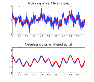
(a) $4\pi^{2}a=0.01,b=0.03$ and $\lambda=1.5$

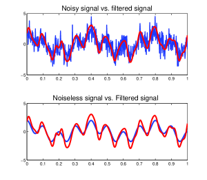
(b) $4\pi^{2}a=0.01,b=0.05$ and $\lambda=1.5$

Figure 10: The red line depicts the filtered signal. In this case, we took $u_{0}(x)=\cos(5\pi x)+\cos(20\pi x)$.

This statement is confirmed by Figure 10(b), where the signal has a medium SNR. We obtain a “good” smoothing and an interesting amplification of the low and medium frequencies.

5 Performance metrics

In this section, we wish to measure the denoising ability of our model. To evaluate our approach and compare it with the Savitzky-Golay filter, we use two measures: the Mean Square Error (MSE) and the Signal-to-Noise Ratio (SNR). These metrics are frequently used in signal processing. They are defined as follows:

$$MSE=\frac{1}{N}\sum_{i=1}^{N}(u_{0}(i)-u(i))^{2}$$

$$SNR_{db}=10\log_{10}\left(\frac{\sum_{i=1}^{N}u_{0}(i)^{2}}{\sum_{i=1}^{N}(u_{0}(i)-u(i))^{2}}\right)$$

where $u_{0}$ is the noiseless original signal, $u$ is the filtered signal and $N$ is the length of the filter.
It is easy to see that a small MSE corresponds to a high noise reduction and that a large SNR indicates a good denoising. To compare the performance of filters, we consider a signal of trigonometric type and an ECG signal. Noise is added to these signals with SNR varying between 0 to 8. Results are plotted in figures 10(a) and 5(b). For each signal, we use a sample of 100 random noises. The performance of the two approaches is estimated using MSE and SNR criteria. We plot an average of the results on figures 11 and 12. Figures 11(a) and 12(a) show SNR values for these two methods applied to trigonometric and electrocardiogram signals. Figures 11(b) and 12(b) show MSE values. These values show the high performance of nonlocal approach in signal denoising for trigonometric signals. Remember that in this case, the algorithm used for the implementation of the equation is the FFT, which is most suitable for trigonometric signals. We may just notice in figure 12 that for high SNR, the Savitzky-Golay filter is better than the nonlocal filter approach. Still, when the SNR is low - and it is the critical case - the proposed method is more efficient than the Savitzky-Golay. Thus, the implementation of our PDE based on the FFT may not be effective for any type of signal, at least when the SNR is high. Alternatively, we may use the finite difference scheme. Results of the filtering are illustrated in figure 13. As we can see, the proposed model is always more efficient than the Savitzky-Golay approach, but for low SNR the FFT scheme remains best. Finally, regardless the type of signal considered, the fractal conservation law (1) is a good tool of denoising, provided that it is implemented with the right method.

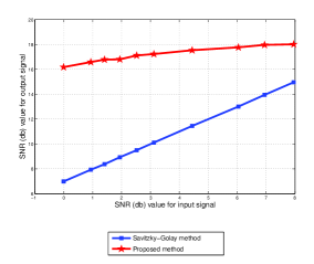
(a) SNR values in Savitzky-Golay method in comparison to proposed method

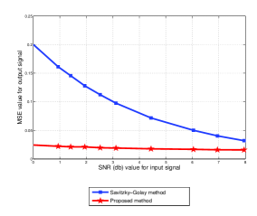
(b) MSE values in Savitzky-Golay method in comparison to proposed method

Figure 11: Choice of parameters: $4\pi^{2}a=0.01,b=0.03$ and $\lambda=1.5$. The initial signal is $u_{0}(x)=\cos(5\pi x)+\cos(20\pi x)$.

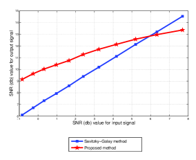
(a) SNR values in Savitzky-Golay method in comparison to proposed method

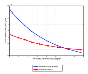
(b) MSE values in Savitzky-Golay method in comparison to proposed method

Figure 12: Choice of parameters: $4\pi^{2}a=0.005,b=0.015$ and $\lambda=1.7$ . The initial signal $u_{0}(x)$ is an electrocardiogram (ECG) signal.

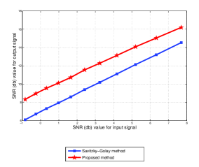
(a) SNR values in Savitzky-Golay method in comparison to proposed method using finite difference scheme

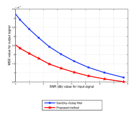
(b) MSE values in Savitzky-Golay method in comparison to proposed method

Figure 13: Choice of parameters: $a=0.5,b=0.3,\lambda=1/3$. The initial signal $u_{0}(x)$ is an electrocardiogram (ECG) signal.

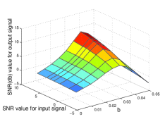
(a)

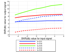
(b)

Figure 14: Choice of parameters: $4\pi^{2}a=0.01$ and $\lambda=1.5$ . The initial signal is $u_{0}(x)=\cos(5\pi x)+\cos(20\pi x)$.

Remark 6.

Let us briefly explain how SNR metrics allow us to optimize the choice of parameter $b$. In figure 14, we display the behaviour of SNR values for different values of $b$. As we can remark, the denoising will be most efficient for $b\approx 0.03$. Hence visualization of the surface (figure 14(a)) and curves (figure 14(b)) enables us to find easily the parameter $b$ for optimal denoising.

6 Concluding remarks

Our first aim was to introduce a fractal conservation law for denoising and contrast enhancement of signals. This device permits to reduce considerably the noise and to increase contrasts simultaneously. The study showed that our filter eliminates the high frequencies and amplifies the low/medium frequencies. In this paper, we also discussed the choice of parameters $a,b$ and $\lambda$.

This equation has been implemented using both a finite difference scheme and the fast Fourier transform. Various well-known measuring metrics have been used to compare our method with the Savitzky-Golay filter. Results showed the good performance of our model. Moreover, the analysis highlighted that, depending on the considered signal, it may be more suitable to use the finite difference scheme or the FFT algorithm when the SNR is high. Obviously, for a sinusoidal type signal, it is preferable to use the FFT, whereas for a signal like step functions it is better to implement the fractal equation with finite difference method. Nevertheless, no matter the algorithm used, the fractal consersation law (1) is an interesting and natural method for denoising and contrast enhancement.

These satisfying properties for signal processing encourages us to implement it for image enhancement: this study is in progress.

7 Acknowledgements

We thank Bijan Mohammadi for advice on numerical schemes and for helpful comments. P. Azerad and A. Bouharguane are supported by the ANR MATHOCEAN ANR-08-BLAN-0301-02.

References

- [1] Alibaud N.; Azerad P.; Isebe D., A non-monotone nonlocal conservation law for dune morphodynamics , Differential and Integral Equations, 23 (2010), pp. 155-188.
- [2] Alvarez-Samaniego B.; Azerad P., Existence of travelling-wave and local well-posedness of the Fowler equation, Disc. Cont. Dyn. Syst., Ser. B, 12 (2009), pp. 671-692.
- [3] Azerad P.; Bouharguane A. , On the stability of a nonlocal conservation law, in preparation.
- [4] Bai J.; Feng X.-C., Fractional-order anisotropic diffusion for image denoising , IEEE Trans. Image Processing, vol. 16, no. 10 (2007), pp. 2492-2502.
- [5] Buadues A.; Bartomeu C.; Morel J.-M., Neighborhood filters and PDE’s, Numerische Mathematik 105 (2006), pp. 1-34.
- [6] Catte F.; Lions P.L; Morel J.-M.; Coll T., Image selective smoothing and edge detection by nonlineal diffusion, SIAM J. Numer. Anal. 29 (1992), pp 182-193.
- [7] Cuesta E.; Kirane M.; Malik S.A., Anisotropic like approach to image denoising by means of generalized fractional time integrals, preprint: http://hal.archives-ouvertes.fr/hal-00437341/fr/.
- [8] Diethelm K.; Ford N.J.; Freed A.D.; Luchko Yu. , Algorithms for the fractional calculus: a selection of numerical methods, Comput. Methods Appl. Mech. Engrg. 194, no. 6-8 (2005), pp. 743-773.
- [9] Droniou J.; Gallouet T.; Vovelle J., Global solution and smothing effect for a non-local regularization of an hyperbolic equation , J. Evol.Eq. 3 (2003), pp. 499-521.
- [10] Droniou J.; Imbert C., Fractal first-order partial differential equations, Arch. Ration. Mech. Anal. 182, no. 2 (2006), pp. 299-331.
- [11] Droniou J., A numerical method for fractal conservation laws, Math. Comp. 79, no. 269 (2010), pp 95-124.
- [12] Fowler A.C., Dunes and drumlins, Geomorphological fluid mechanics, eds. A. Provenzale and N. Balmforth, Springer-Verlag, Berlin, 211 (2001), pp. 430-454.
- [13] Fowler A.C., Evolution equations for dunes and drumlins, Rev. R. Acad. de Cien, Serie A. Mat, 96 (3) (2002), pp. 377-387.
- [14] Fowler A.C, Mathematics and the environment, lecture notes http://www2.maths.ox.ac.uk/~fowler/courses/mathenvo.html.
- [15] Guidotti P., A new nonlocal nonlinear diffusion of image processing, J. Differential Equations 246, no. 12 (2009), pp. 4731-4742.
- [16] Imbert C., A non-local regularization of first order Hamilton-Jacobi equations, J. Differential Equations 211, no. 1 (2005), pp. 218-246.
- [17] Kouakou K.K.J.; Lagree P-Y, Evolution of a model dune in a shear flow, Eur. J. Mech. B Fluids, 25 no. 3 (2006), pp 348-359.
- [18] Lagree P-Y; Kouakou K. , Stability of an erodible bed in various shear flows, European Physical Journal B - Condensed matter, Vol. 47 (2005), pp 115-125.
- [19] Mohammadi B.; Saiac J-H , Pratique de la simulation numérique, Dunod: Paris (2003).
- [20] Nikpour M.; Nadernejad E.; Ashtiani H.; Hassanpour H. , Using PDE’s for Noise Reduction in Time Series , International Journal of computing and ICT Research, Vol. 3, No. 1 (2009).
- [21] Peiro J.; Sherwin S.,Finite difference, finite element and finite volume methods for partial differential equations, Handbook of Materials Modeling. Volume 1 (2005): Methods and Models, pp. 1-32.
- [22] Perona P.; Malik J., Scale-space and edge detection using anistropic diffusion, IEEE Transactions on Pattern Analysis and Machine Intelligence 12(7) (1990), pp. 626-639.
- [23] Podlubny I., An introduction to fractional derivatives, fractional differential equations, to methods of their solution and some of their applications., Mathematics in Science and Engineering, 198 Academic Press, San Diego, (1999).
- [24] Savitzky A.; Golay M.J.E., Smoothing and Differentiation of Data by Simplified Least Squares Procedures, Analytical Chemistry 36 (8) (1964).