Massive star formation in Wolf-Rayet galaxies

Abstract

Context. We have performed a comprehensive multiwavelength analysis of a sample of 20 starburst galaxies that show a substantial population of very young massive stars, most of them classified as Wolf-Rayet (WR) galaxies.

Aims. We have analysed optical/NIR colours, physical and chemical properties of the ionized gas, stellar, gas and dust content, star-formation rate and interaction degree (among many other galaxy properties) of our galaxy sample using multi-wavelength data. We compile 41 independent star-forming regions –with oxygen abundances between 12+log(O/H)= 7.58 and 8.75–, of which 31 have a direct estimate of the electron temperature of the ionized gas.

Methods. This paper, only submitted to astro-ph, compiles the most common empirical calibrations to the oxygen abundance, and presents the comparison between the chemical abundances derived in these galaxies using the direct method with those obtained through empirical calibrations, as it is published in López-Sánchez & Esteban (2010b).

Results. We find that (i) the Pilyugin method (Pilyugin 2001a,b; Pilyugin & Thuan 2005), which considers the $R_{23}$ and the $P$ parameters, is the best suited empirical calibration for these star-forming galaxies, (ii) the relations between the oxygen abundance and the $N_{2}$ or the $O_{3}N_{2}$ parameters provided by Pettini & Pagel (2004) give acceptable results for objects with 12+log(O/H)$>$8.0, and (iii) the results provided by empirical calibrations based on photoionization models (McGaugh, 1991; Kewley & Dopita, 2002; Kobulnicky & Kewley, 2004) are systematically 0.2 – 0.3 dex higher than the values derived from the direct method. These differences are of the same order that the abundance discrepancy found between recombination and collisionally excited lines. This may suggest the existence of temperature fluctuations in the ionized gas, as exists in Galactic and other extragalactic H ii regions.

Conclusions. All these results are included in the paper Massive Star Formation in Wolf-Rayet galaxies IV. Colours, chemical-composition analysis and metallicity-luminosity relations, López-Sánchez & Esteban (2010b), A&A, in press (Sect. 4.4 and Appendix A). Please, if this information is used, reference that paper and NOT this document, which have been only submitted to astro-ph to emphasize these results.

1 Introduction

The knowledge of the chemical composition of galaxies, in particular of dwarf galaxies, is vital for understanding their evolution, star formation history, stellar nucleosynthesis, the importance of gas inflow and outflow, and the enrichment of the intergalactic medium. Indeed, metallicity is a key ingredient for modelling galaxy properties, because it determines UV, optical and NIR colours at a given age (i.e., Leitherer et al. 1999), nucleosynthetic yields (e.g., Woosley & Weaver 1995), the dust-to-gas ratio (e.g., Hirashita et al 2001), the shape of the interstellar extinction curve (e.g., Piovan et al. 2006), or even the properties of the Wolf-Rayet stars (Crowther, 2007).

The most robust method to derive the metallicity in star-forming and starburst galaxies is via the estimate of metal abundances and abundance ratios, in particular through the determination of the gas-phase oxygen abundance and the nitrogen-to-oxygen ratio. The relationships between current metallicity and other galaxy parameters, such as colours, luminosity, neutral gas content, star-formation rate, extinction or total mass, constrain galaxy-evolution models and give clues about the current stage of a galaxy. For example, is still debated whether massive star formation results in the instantaneous enrichment of the interstellar medium of a dwarf galaxy, or if the bulk of the newly synthesized heavy elements must cool before becoming part of the interstellar medium (ISM) that eventually will form the next generation of stars. Accurate oxygen abundance measurements of several H ii regions within a dwarf galaxy will increase the understanding of its chemical enrichment and mixing of enriched material.

Furthermore, today it is the metallicity (which reflects the gas reprocessed by stars and any exchange of gas between the galaxy and its environment) and not the stellar mass (which reflects the amount of gas locked up into stars) of a galaxy the main problem to get a proper metallicity-luminosity relation, so that different methods involving direct estimates of the oxygen abundance, empirical calibrations using bright emission-line ratios or theoretical methods based on photoionization models yield very different values (i.e., Yin et al. 2007; Kewley & Elisson, 2008).

Hence precise photometric and spectroscopic data, including a detailed analysis of each particular galaxy that allows conclusions about its nature, are crucial to address these issues. We performed such a detailed photometric and spectroscopic study in a sample of strong star-forming galaxies, many of them previously classified as dwarf galaxies. The majority of these objects are Wolf-Rayet (WR) galaxies, a very inhomogeneous class of star-forming objects which share at least an ongoing or recent star formation event that has produced stars sufficiently massive to evolve into the WR stage (Schaerer, Contini & Pindao, 1999). The main aim of our study of the formation of massive stars in starburst galaxies and the role that the interactions with or between dwarf galaxies and/or low surface brightness objects have in its triggering mechanism. In Paper I (López-Sánchez & Esteban, 2008) we described the motivation of this work, compiled the list of the 20 analysed WR galaxies (Table 1 of Paper I), the majority of them showing several sub-regions or objects within or surrounding them, and presented the results of the optical/NIR broad-band and H$\alpha$ photometry. In Paper II (López-Sánchez & Esteban, 2009) we presented the results of the analysis of the intermediate resolution long-slit spectroscopy of 16 WR galaxies of our sample – the results for the other four galaxies were published separately, see López-Sánchez, Esteban & Rodríguez (2004a, b); López-Sánchez, Esteban & García-Rojas (2006); López-Sánchez et al. (2007). In many cases, two or more slit positions were used to analyse the most interesting zones, knots or morphological structures belonging to each galaxy or even surrounding objects. Paper III (López-Sánchez & Esteban, 2010a) presented the analysis of the O and WR stellar populations within these galaxies. Paper IV (López-Sánchez & Esteban, 2010b) globally compile and analyse the optical/NIR photometric data and study the physical and chemical properties of the ionized gas within our galaxy sample. The results shown in this paper haven been already published in Paper IV. The final paper of the series (Paper V; López-Sánchez 2010) compiles the properties derived with data from other wavelengths (UV, FIR, radio, and X-ray) and complete a global analysis of all available multiwavelength data of our WR galaxy sample. We have produced the most comprehensive data set of these galaxies so far, involving multiwavelength results and analysed according to the same procedures.

2 Empirical calibrations of the oxygen abundance

When the spectrum of an extragalactic H ii region does not show the [O iii] $\lambda$4363 emission line or other auroral lines that can be used to derive $T_{\rm e}$, the so-called empirical calibrations are applied to get a rough estimation of its metallicity. Empirical calibrations are inspired partly by photo-ionization models and partly by observational trends of line strengths with galactocentric distance in gas-rich spirals, which are believed to be due to a radial abundance gradient with abundances decreasing outwards. In extragalactic objects, the usefulness of the empirical methods goes beyond the derivation of abundance gradients in spirals (Pilyugin, Vílchez & Contini, 2004), as these methods find application in chemical abundance studies of a variety of objects, including low-surface brightness galaxies (de Naray, McGaugh & de Blok, 2004) and star-forming galaxies at intermediate and high redshift, where the advent of 8–10 m class telescopes has made it possible to extend observations (e.g., Teplitz et al. 2000, Pettini et al. 2001; Kobulnicky et al 2003; Lilly, Carollo & Stockton 2003; Steidel et al. 2004; Kobulnicky & Kewley 2004; Erb et al. 2006).

As the brightest metallic lines observed in spectra of H ii regions are those involving oxygen, this element has been extensively used to get a suitable empirical calibration. Oxygen abundance is important as one of the fundamental characteristics of a galaxy: its radial distribution is combined with radial distributions of gas and star surface mass densities to constrain models of chemical evolution. Parameters defined in empirical calibrations evolving bright oxygen lines are

$$R_{3}=\frac{I([{\rm O\,III}])\lambda 4959+I([{\rm O\,III}])\lambda 5007}{\rm H\beta},$$ (1)

$$R_{2}=\frac{I([{\rm O\,II}])\lambda 3727}{\rm H\beta},$$ (2)

$$R_{23}=R_{3}+R_{2},$$ (3)

$$P=\frac{R_{3}}{R_{23}},$$ (4)

$$y=\log\frac{R_{3}}{R_{2}}=\log\frac{1}{P^{-1}-1}.$$ (5)

Jensen, Strom & Strom (1976) presented the first exploration in this method considering the $R_{3}$ index, which considers the [O iii] $\lambda\lambda$4959,5007 emission lines. However, were Pagel et al. (1979) who introduced the most widely used abundance indicator, the $R_{23}$ index, which also included the bright [O ii] $\lambda$3727 emission line. Since then, many studies have been performed to refine the calibration of $R_{23}$ (Edmunds & Pagel, 1984; McCall, Rybski & Shields,, 1985; Dopita & Evans, 1986; Torres-Peimbert et al., 1989; McGaugh, 1991; Zaritsky, Kennicutt & Huchra, 1994; Pilyugin, 2000, 2001a, 2001b; Kewley & Dopita, 2002; Kobulnicky & Kewley, 2004; Pilyugin & Thuan, 2005; Nagao, Maiolino & Marconi, 2006). The most successful are the calibrations of McGaugh (1991) and Kewley & Dopita (2002), which are based on photoionization models, and the empirical relations provided by Pilyugin (2001a, b) and Pilyugin & Thuan (2005). Both kinds of calibrations improve the accuracy by making use of the [O iii]/[O ii] ratio as ionization parameter, which accounts for the large scatter found in the $R_{23}$ versus oxygen abundance calibration, which is larger than observational errors (Kobulnicky, Kennicutt & Pizagno, 1999). Figure 1 shows the main empirical calibrations that use the $R_{23}$ parameter.

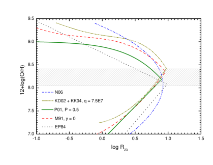
Figure 1: Empirical calibrations of oxygen abundance using the $R_{23}$ parameter. Note that they are bi-valuated. The dashed zone indicates the region with higher uncertainties in O/H. The empirical calibrations plotted in the figure are: EP94: Edmund & Pagel (1984); M91: McGaugh (1991) using $y$=0 ($R_{2}=R_{3}$); P01: Pilyugin (2001) using $P=0.5$ ($R_{2}=R_{3}$); (KD02+KK04): Kewley & Dopita (2002) using the formulation of Kobulnicky & Kewley (2004) assuming $q=7.5\times 10^{7}$ cm s^-1; N06: Nagao et al. (2006) using their cubic fit to $R_{23}$.

The main problem associated with the use of $R_{23}$ parameter is that it is bivaluated, i.e., a single value of $R_{23}$ can be caused by two very different oxygen abundances. The reason of this behaviour is that the intensity of oxygen lines does not indefinitely increase with metallicity. Thus, there are two branches for each empirical calibration (see Fig. 1): the low-metallicity regime, with 12+log(O/H)$\leq$8.1, and the high-metallicity regime, with 12+log(O/H)$\geq$8.4. That means that a very large fraction of the star-forming regions lie in the ill-defined turning zone around 12+log(O/H)$\simeq$8.20, where regions with the same $R_{23}$ value have oxygen abundances that differ by almost an order of magnitude. Hence, additional information, such as the [N ii]/H$\alpha$ or the [O ii]/[O iii] ratios, is needed to break the degeneracy between the high and low branches (i.e., Kewley & Dopita, 2002). Besides, the $R_{23}$ method requires that spectrophotometric data are corrected by reddening, which effect is crucial because [O ii] and [O iii] lines have a considerably separation in wavelength.

Here we list all empirical calibrations that were considered in this work, compiling the equations needed to derive the oxygen abundance from bright emission line ratios following every method.

Edmund & Pagel (1984): Although the $R_{23}$ parameter was firstly proposed by Pagel et al. (1979), the first empirical calibration was given by Edmunds & Pagel (1984),

$$12+\log({\rm O/H})_{up}=8.76-0.69\log R_{23},$$

$$12+\log({\rm O/H})_{low}=6.43+1.67\log R_{23},$$ (6)

with the limit between the lower and the upper branches at 12+log(O/H)$\sim$8.0.

McCall, Rybski & Shields (1985) presented an empirical calibration for oxygen abundance using the $R_{23}$ parameter, only valid for 12+log(O/H)$>$8.15. However, they did not give an analytic formulae but only listed it numerically (see their Table 15). The four-order polynomical fit for their values gives the following relation:

$$12+\log({\rm O/H})_{up}= 9.32546-0.360465x+0.203494x^{2} +0.278702x^{3}-1.36351x^{4},$$ (7)

with $x=\log R_{23}$.

Zaritzky, Kennicutt & Huchra (1994) provided a simple analytic relation between oxygen abundance and $R_{23}$:

$$12+\log({\rm O/H})_{up}=9.265-0.33x-0.202x^{2}-0.207x^{3}-0.333x^{4}.$$ (8)

Their formula is an average of three previous calibrations: Edmunds & Pagel (1984), McCall et al. (1985) and Dopita & Evans (1986). Following the authors, this calibration is only suitable for 12+log(O/H)$>$8.20, but perhaps a more realistic lower limit is 8.35.

McGaugh (1991) calibrated the relationship between the $R_{23}$ ratio and gas-phase oxygen abundance using H ii region models derived from the photoionization code Cloudy (Ferland et al., 1998). McGaugh’s models include the effects of dust and variations in ionization parameter, $y$. Kobulnicky et al. (1999) give analytical expressions for the McGaugh (1991) calibration based on fits to photoionization models; the middle point between both branches is 12+log(O/H)$\sim$8.4:

$$12+\log({\rm O/H})_{up}= 7.056+0.767x+0.602x^{2}-y(0.29+0.332x-0.331x^{2}),$$ (9)

$$12+\log({\rm O/H})_{low}= 9.061-0.2x-0.237x^{2}-0.305x^{3}-0.0283x^{4}$$ (10)

$$-y(0.0047-0.0221x-0.102x^{2}-0.0817x^{3}-0.00717x^{4}).$$

Pilyugin (2000) found that the previous calibrations using the $R_{23}$ parameter had a systematic error depending on the hardness of the ionizing radiation, suggesting that the excitation parameter, $P$, is a good indicator of it. In several papers, Pilyugin performed a detailed analysis of the observational data combined with photoionization models to obtain empirical calibrations for the oxygen abundance. Pilyugin (2000) confirmed the idea of McGaugh (1991) that the strong lines of [O ii] and [O iii] contain the necessary information for the determination of accurate abundances in low-metallicity (and may be also in high-metallicity) H ii regions. He used new observational data to propose a linear fit involving only the $R_{23}$ parameter,

$$12+\log({\rm O/H})_{up}=9.50-1.40\log R_{23},$$ (11)

$$12+\log({\rm O/H})_{low}=6.53+1.40\log R_{23},$$ (12)

assuming a limit of 12+log(O/H)$\sim$8.0 between the two branches. This calibration is close to that given by Edmunds & Pagel (1984); it has the same slope, but Pilyugin (2000) is shifted towards lower abundances by around 0.07 dex. However, this new relation is not sufficient to explain the wide spread of observational data. Thus, Pilyugin (2001a) give the following, more real and complex, calibration involving also the excitation parameter $P$:

$$12+\log({\rm O/H})_{up}=\frac{R_{23}+54.2+59.45P+7.31P^{2}}{6.01+6.71P+0.371P^{2}+0.243R_{23}}.$$ (13)

This is the so-called P-method, which can be used in moderately high-metallicity H ii regions (12+log(O/H)$\geq$8.3). Pilyugin used two-zone models of H ii regions and assumed the $T_{e}$(O ii) – $T_{e}$(O iii) relation from Garnett (1992). For the low metallicity branch, Pilyugin (2001b) found that

$$12+\log({\rm O/H})_{low}=6.35+1.45\log R_{23}-1.74\log P.$$ (14)

Pilyugin estimates that the precision of oxygen abundance determination with this method is around 0.1 dex.

Pilyugin & Thuan (2005) revisited these calibrations including more spectroscopic measurements of H ii regions in spiral and irregular galaxies with a measured intensity of the [O iii] $\lambda$4363 line and recalibrate the relation between the oxygen abundance and the $R_{23}$ and $P$ parameters, yielding to:

$$12+\log({\rm O/H})_{low}=\frac{R_{23}+106.4+106.8P-3.40P^{2}}{17.72+6.60P+6.95P^{2}-0.302R_{23}},$$ (15)

$$12+\log({\rm O/H})_{up}=\frac{R_{23}+726.1+842.2P+337.5P^{2}}{85.96+82.76P+43.98P^{2}+1.793R_{23}}.$$ (16)

Kewley & Dopita (2002) used a combination of stellar population synthesis and photoionization models to develop a set of ionization parameters and abundance diagnostic based only on the strong optical emission lines. Their optimal method uses ratios of [N ii], [O ii], [O iii], [S ii], [S iii] and Balmer lines, which is the full complement of strong nebular lines accessible from the ground. They also recommend procedures for the derivation of abundances in cases where only a subset of these lines is available. Kewley & Dopita (2002) models start with the assumption that $R_{23}$, and many of the other emission-line abundance diagnostics, also depends on the ionization parameter $q\equiv c\times U$, that has units of cm s^-1. They used the stellar population synthesis codes Starburst 99 (Leitherer et al., 1999; Vázquez & Leitherer, 2005) and Pegase.2 (Fioc & Rocca-Volmerange, 1997) to generate the ionizing radiation field, assuming burst models at zero age with a Salpeter IMF and lower and upper mass limits of 0.1 and 120 $M_{\odot}$, respectively, with metallicities between 0.05 and 3 times solar. The ionizing radiation fields were input into the photoionization and shock code, Mappings (Sutherland & Dopita, 1993), which includes self-consistent treatment of nebular and dust physics. Kewley & Dopita (2002) previously used these models to simulate the emission-line spectra of H ii regions and starburst galaxies (Dopita et al., 2000), and are completely described in their study.

Kobulnicky & Kewley (2004) gave a parameterization of the Kewley & Dopita (2002) $R_{23}$ method with a form similar to that given by McGaugh (1991) calibration. Kobulnicky & Kewley (2004) presented an iterative scheme to resolve for both the ionization parameter $q$ and the oxygen abundance using only [O iii], [O ii] and H$\beta$ lines. The parameterization they give for $q$ is

$$\log(q)=\frac{32.81-1.153y^{2}+\big{[}12+\log({\rm O/H})\big{]}\big{[}-3.396-0.025y+0.1444y^{2}\big{]}}{4.603-0.3119y-0.163y^{2}+\big{[}12+\log({\rm O/H})\big{]}\big{[}-0.48+0.0271y+0.02037y^{2}\big{]}},$$ (17)

where $y=\log$([O iii]/[O ii]). This equation is only valid for ionization parameters between 5$\times$10⁶ and 1.5$\times$10⁸ cm s^-1. The oxygen abundance is parameterized by

$$12+\log({\rm O/H})_{up}=9.72-0.777x-0.951x^{2}-0.072x^{3}-0.811x^{4}-\log(q)$$

$$\times(0.0737-0.0713x-0.141x^{2}+0.0373x^{3}-0.058x^{4}),$$ (18)

$$12+\log({\rm O/H})_{low}=9.40+4.65x-3.17x^{2}-\log(q)(0.272+0.547x-0.513x^{2}),$$ (19)

being $x=\log R_{23}$. The first equation is valid for 12+log(O/H)$\geq$8.4, while the second for 12+log(O/H)$<$8.4. Typically, between two and three iterations are required to reach convergence. Following the authors, this parameterization should be regarded as an improved, implementation-friendly approach to be preferred over the tabulated $R_{23}$ coefficients given by Kewley & Dopita (2002).

Nagao, Maiolino & Marcani (2006) did not consider any ionization parameter. They merely used data of a large sample of galaxies from the Sloan Digital Sky Survey (SDSS; York et al. 2000) to derive a cubic fit to the relation between $R_{23}$ and the oxygen abundance,

$$\log R_{23}=1.2299-4.1926y+1.0246y^{2}-0.063169y^{3},$$ (20)

with $y$=12+log(O/H).

Besides $R_{23}$, additional parameters have been used to derive metallicities in star-forming galaxies. Without other emission lines, the $N_{2}$ parameter, which is defined by

$$N_{2}\equiv\log\frac{I([{\rm N\,II}])\lambda 6583}{\rm H\alpha},$$ (21)

can be used as a crude estimator of metallicity. However, we note that the [N ii]/H$\alpha$ ratio is particularly sensitive to shock excitation or a hard radiation field from an AGN. The $N_{2}$ parameter was firstly suggested by Storchi-Bergmann, Calzetti & Kinney (1994), who gave a tentative calibration of the oxygen abundance using this parameter. This calibration has been revisited by van Zee, Salzer & Haynes (1998); Denicoló, Terlevich & Terlevich (2002); Pettini & Pagel (2004) and Nagao et al. (2006). The Denicoló et al. (2002) calibration is

$$12+\log({\rm O/H})=9.12+0.73N_{2},$$ (22)

which considerably improves the previous relations because of the inclusion of an extensible sample of nearby extragalactic H ii regions. The uncertainty of this method is $\sim$0.2 dex because $N_{2}$ is sensitive to ionization and O/N variations, so strictly speaking it should be used mainly as an indicator of galaxy-wide abundances. Denicoló et al. (2002) also compared their method with photoionization models, concluding that the observed $N_{2}$ is consistent with nitrogen being a combination of both primary and secondary origin.

Pettini & Pagel (2004) revisited the relation between the $N_{2}$ parameter and the oxygen abundance including new data for the high- and low-metallicity regimen. They only considered those extragalactic H ii regions where the oxygen values are determined either via the $T_{e}$ method or with detailed photoionization modelling. The linear fit to their data is

$$12+\log({\rm O/H})=8.90+0.57N_{2},$$ (23)

which has both a lower slope and zero-point that the fit given by Denicoló et al. (2002). A somewhat better relation is provided by a third-order polynomical fit of the form

$$12+\log({\rm O/H})=9.37+2.032N_{2}+1.26(N_{2})^{2}+0.32(N_{2})^{3},$$ (24)

valid in the range $-2.5<N_{2}<-0.3$. Nagao et al. (2006) also provided a relation between $N_{2}$ and the oxygen abundance, their cubic fit to their SDSS data yields

$$\log N_{2}=96.641-39.941y+5.2227y^{2}-0.22040y^{3},$$ (25)

with $y$=12+log(O/H).

Pettini & Pagel (2004) revived the O₃N₂ parameter, previously introduced by Alloin et al. (1979) and defined by

$$O_{3}N_{2}\equiv\log\frac{[{\rm O\,III}]\ \lambda 5007/{\rm H\beta}}{[{\rm N\,II}]\ \lambda 6583/{\rm H\alpha}}.$$ (26)

Pettini & Pagel (2004) derived the following least-square linear fit to their data:

$$12+\log({\rm O/H})=8.73-0.32O_{3}N_{2}.$$ (27)

Nagao et al. (2006) also revisited this calibration and derived a cubic fit between the O₃N₂ parameter and the oxygen abundance,

$$\log O_{3}N_{2}=-232.18+84.423y-9.9330y^{2}+0.37941y^{3},$$ (28)

with $y$=12+log(O/H).

Other important empirical calibrations that were not used in this study involve the $S_{23}$ parameter, introduced by Vílchez & Esteban (1996) and revisited by Díaz & Pérez-Montero (2000); Oey & Shields (2000) and Pérez-Montero & Díaz (2005). In the last years, bright emission line ratios such as [Ar iii]/[O iii] and [S iii]/[O iii] (Stasińska, 2006) or [Ne iii]/[O iii] and [O iii]/[O ii] (Nagao et al., 2006) have been explored as indicators of the oxygen abundance in H ii regions and starburst galaxies. Peimbert et al. (2007) suggested to use the oxygen recombination lines to get a more precise estimation of the oxygen abundance. Nowadays, there is still a lot of observational and theoretical work to do involving empirical calibrations (see recent review by Kewley & Ellison 2008), but these methods should be used only for objects whose H ii regions have the same structural properties as those of the calibrating samples (Stasińska, 2009).

Table 1: List of the parameters used to compute the oxygen abundance in all regions with a direct estimation of $T_{\rm e}$ using empirical calibrations.

Region	$R_{23}$	$P=R_{3}/R_{23}$	$y$ =log($R_{3}/R_{2}$)	$N_{2}$	$O_{3}N_{2}$	$q_{KD02o}$a
HCG 31 AC	5.42	0.571	0.125	0.104	1.349	3.76E+07
HCG 31 B	7.93	0.408	-0.162	0.101	1.381	4.91E+07
HCG 31 E	7.12	0.511	0.020	0.090	1.486	7.40E+07
HCG 31 F1	8.91	0.819	0.656	0.034	2.201	5.78E+07
HCG 31 F2	7.60	0.724	0.418	0.036	2.064	6.28E+07
HCG 31 G	8.20	0.499	-0.002	0.106	1.462	6.96E+07
Mkn 1199 C	7.69	0.809	0.627	0.131	1.555	1.55E+08
Haro 15 A	9.73	0.884	0.881	0.027	2.378	8.55E+07
Mkn 5 A1	7.58	0.748	0.473	0.051	1.915	6.96E+07
Mkn 5 A2	8.19	0.702	0.372	0.049	1.944	1.72E+08
IRAS 08208+2816 C	7.77	0.793	0.583	0.129	1.558	8.55E+07
POX 4	10.68	0.906	0.986	0.015	2.697	1.05E+08
UM 420	6.45	0.649	0.268	0.099	1.497	4.81E+07
SBS 0926+606A	7.40	0.811	0.632	0.026	2.227	6.68E+07
SBS 0948+532	8.85	0.874	0.843	0.022	2.430	2.54E+08
SBS 1054+365	9.33	0.893	0.920	0.020	2.503	9.10E+07
SBS 1211+540	7.22	0.892	0.918	0.008	2.788	1.16E+08
SBS 1319+579A	9.92	0.908	0.996	0.014	2.671	1.05E+08
SBS 1319+579B	7.13	0.722	0.415	0.046	1.922	6.15E+07
SBS 1319+579C	7.11	0.710	0.389	0.052	1.860	5.91E+07
SBS 1415+437C	5.22	0.783	0.558	0.015	2.301	5.91E+07
SBS 1415+437A	4.86	0.810	0.629	0.012	2.370	5.44E+07
III Zw 107 A	7.13	0.701	0.369	0.100	1.573	5.78E+07
Tol 9 INT	4.58	0.689	0.345	0.252	0.973	4.16E+07
Tol 9 NOT	4.78	0.629	0.230	0.287	0.894	3.39E+07
Tol 1457-262A	9.89	0.773	0.532	0.033	2.236	9.91E+07
Tol 1457-262B	9.00	0.792	0.582	0.020	2.417	1.41E+08
Tol 1457-262C	8.88	0.669	0.359	0.036	2.099	7.16E+07
ESO 566-8	5.17	0.505	0.008	0.414	0.693	3.19E+07
NGC 5253 A	9.20	0.851	0.756	0.102	1.754	6.82E+07
NGC 5253 B	9.38	0.856	0.775	0.086	1.841	7.11E+07
NGC 5253 C	8.03	0.773	0.532	0.041	2.046	2.60E+08
NGC 5253 D	7.67	0.527	0.048	0.079	1.582	7.72E+07

^a Value derived for the $q$ parameter (in units of cm s^-1) obtained using the optimal calibration given by Kewley & Dopita (2002).

Table 2: Results of the oxygen abundance, in the form 12+log(O/H), for objects with a direct estimation of the metallicity, considering several empirical calibrations.

Region	Branch	$T_{\rm e}$	EP84	MRS85	M91	ZKH94	P00	P01a	PT05b	KD02	KK04	D02	PP04a	PP04b	PP04c	N06ac	N06b	N06c
			R23	R23	R23, $y$	R23	R23	R23, P	R23, P	R23, $q$	R23, $q$	N2	N2	N2	O3N2	R23	N2	O3N2
HCG 31 AC	H	8.22$\pm$0.05	8.25	8.89	8.67	8.74	8.47	8.15	8.09	7.99	8.12	8.40	8.34	8.29	8.30	8.05	8.16	8.22
HCG 31 B	H	8.14$\pm$0.08	8.14	8.48	8.29	8.44	8.24	8.22	8.12	8.41	8.44	8.39	8.33	8.28	8.29	8.07	8.16	8.20
HCG 31 E	H	8.13$\pm$0.09	8.17	8.62	8.14	8.53	8.31	8.18	8.13	8.19	8.32	8.35	8.30	8.26	8.25	8.07	8.11	8.15
HCG 31 F1	L	8.07$\pm$0.06	8.02	8.30	8.13	…	7.86	8.12	7.99	8.46	8.33	8.05	8.07	8.09	8.03	…	7.81	7.67
HCG 31 F2	L	8.03$\pm$0.10	7.90	8.54	8.06	8.48	7.76	8.13	7.95	8.19	8.27	8.06	8.07	8.10	8.07	8.07	7.83	7.79
HCG 31 G	H	8.15$\pm$0.08	8.13	8.43	8.26	8.40	8.22	8.11	8.17	8.31	8.42	8.41	8.34	8.29	8.26	8.07	8.17	8.16
Mkn 1199 C	H	8.75$\pm$0.12	9.37	9.26	9.00	9.18	9.19	8.71	8.54	9.14	9.14	8.92	8.74	8.90	8.81	9.18	8.78	8.94
Haro 15 A	H	8.10$\pm$0.06	8.08	…	8.14	…	7.91	8.12	8.12	8.48	8.34	7.98	8.01	8.05	7.97	…	7.74	7.38
Mkn 5 A1	L	8.07$\pm$0.07	7.90	8.54	8.04	8.48	7.76	8.13	8.13	8.19	8.26	8.18	8.17	8.16	8.12	8.07	7.94	7.89
Mkn 5 A2	L	8.08$\pm$0.07	7.95	8.43	8.14	8.41	7.81	7.92	8.17	8.18	8.33	8.16	8.15	8.15	8.11	8.07	7.92	7.87
IRAS 08208+2816	H	8.33$\pm$0.08	8.15	8.50	8.55	8.46	8.25	8.42	8.35	8.35	8.25	8.47	8.39	8.34	8.23	8.35	8.23	8.11
POX 4	L	8.03$\pm$0.04	8.15	…	8.20	…	7.97	7.92	8.06	8.48	8.40	7.78	7.86	7.91	7.87	…	7.53	…
UM 420	L	7.95$\pm$0.05	7.78	8.73	7.98	8.61	7.66	7.85	7.86	8.02	8.16	8.20	8.39	8.33	8.28	7.57	8.15	8.14
SBS 0926+606A	L	7.94$\pm$0.08	7.88	8.57	7.97	8.50	7.75	7.77	7.80	8.17	8.20	7.97	8.00	8.05	8.02	7.71	7.73	7.64
SBS 0948+532	L	8.03$\pm$0.05	8.01	8.31	8.06	…	7.86	7.82	8.10	8.34	8.28	7.91	7.95	8.01	7.95	…	8.01	…
SBS 1054+365	L	8.00$\pm$0.07	8.05	8.21	8.09	…	7.89	7.84	7.91	8.48	8.30	7.87	7.93	7.98	7.93	…	7.63	…
SBS 1211+540	L	7.65$\pm$0.04	7.86	8.60	7.85	8.52	7.73	7.68	7.65	8.02	8.10	7.58	7.70	7.69	7.84	7.68	7.31	…
SBS 1319+579A	L	8.05$\pm$0.06	8.09	…	8.13	…	7.93	8.11	8.11	8.48	8.33	7.77	7.85	7.90	7.88	…	7.52	…
SBS 1319+579B	L	8.12$\pm$0.10	7.85	8.62	8.01	8.53	7.72	8.13	8.12	8.13	8.23	8.14	8.14	8.14	8.11	8.07	7.90	7.89
SBS 1319+579 C	L	8.15$\pm$0.07	7.85	8.62	8.02	8.53	7.72	8.13	8.13	8.12	8.23	8.18	8.17	8.16	8.13	8.06	7.94	7.93
SBS 1415+437 C	L	7.58$\pm$0.05	7.63	8.91	7.72	8.76	7.53	7.57	7.55	7.86	7.99	7.79	7.86	7.92	7.99	7.39	7.55	7.55
SBS 1415+437 A	L	7.61$\pm$0.06	7.58	8.96	7.64	8.80	7.49	7.50	7.48	7.82	7.92	7.72	7.81	7.86	7.97	7.34	7.48	7.41
III Zw 107	H	8.23$\pm$0.09	8.17	8.62	8.57	8.53	8.31	8.40	8.35	8.13	8.24	8.39	8.33	8.28	8.23	8.46	8.15	8.10
Tol 9 INT	H	8.58$\pm$0.15	8.30	9.00	8.76	8.84	8.58	8.61	8.55	8.95	8.90	8.68	8.56	8.54	8.42	8.77	8.46	8.40
Tol 9 NOT	H	8.55$\pm$0.16	8.29	8.97	8.73	8.81	8.55	8.56	8.50	8.94	8.88	8.72	8.59	8.59	8.44	8.75	8.51	8.44
Tol 1457-262A	L	8.05$\pm$0.07	8.09	…	8.26	…	7.92	8.11	8.20	8.58	8.42	8.04	8.06	8.09	8.02	…	7.80	7.63
Tol 1457-262B	L	7.88$\pm$0.07	8.55	…	8.21	…	7.87	7.91	8.21	8.38	8.29	7.88	7.93	7.99	7.96	…	7.60	…
Tol 1457-262C	L	8.06$\pm$0.11	8.48	…	8.21	…	7.88	8.00	8.24	8.48	8.37	8.07	8.08	8.10	8.06	…	7.83	7.77
ESO 566-8	H	8.46$\pm$0.11	8.27	8.92	8.68	8.77	8.50	8.44	8.38	8.92	8.84	8.84	8.68	8.76	8.51	8.70	8.66	8.53
NGC 5253 A	H	8.18$\pm$0.04	8.09	8.24	8.13	…	8.15	8.11	8.13	8.53	8.33	8.40	8.34	8.28	8.17	…	8.16	8.00
NGC 5253 B	H	8.19$\pm$0.04	8.09	8.21	8.14	…	8.14	8.11	8.13	8.48	8.34	8.34	8.29	8.25	8.14	…	8.10	7.94
NGC 5253 C	L	8.28$\pm$0.04	8.14	8.46	8.53	8.42	8.23	8.38	8.32	8.67	8.63	8.11	8.11	8.13	8.08	8.30	7.87	7.80
NGC 5253 D	L	8.31$\pm$0.07	8.15	8.52	8.19	8.47	8.26	8.23	8.17	8.32	8.37	8.31	8.27	8.23	8.22	8.37	8.07	8.10

NOTE: The empirical calibrations and the parameters used for each of them are: EP84: Edmunds & Pagel (1984) that involves the $R_{23}$ parameter; MRS85: McCall, Rybski & Shields (1985) using $R_{23}$; M91: McGaugh (1991) using $R_{23}$ and $y$; ZKH94: Zaritzky, Kennicutt & Huchra (1994) using $R_{23}$; P00: Pilyugin (2000) using $R_{23}$; P01: Pilyugin (2001a,b) using $R_{23}$ and $P$; KD02: Kewley & Dopita (2002) using $R_{23}$ and $q$; KK04: Kobulnicky & Kewley (2004) using $R_{23}$ & $q$; D02: Denicoló, Terlevich & Terlevich (2002) using the $N_{2}$ parameter; PP04: Pettini & Pagel (2004), using (a) $N_{2}$ with a linear fit, (b) $N_{2}$ with a cubic fit, (c) the $O_{3}N_{2}$ parameter; N06: Nagao et al. (2006) using the cubic relations involving the $R_{23}$ (a), $N_{2}$ (b) and $O_{3}N_{2}$ (c) parameters. The value compiled in the column labeled $T_{\rm e}$ is the oxygen abundance derived by the direct method.

^a The value listed for P01 is the average value between the high- and the low-metallicity branches for objects with 7.90$<$12+log(O/H)$<$8.20.

^b The value listed for PT05 is the average value between the high- and the low-metallicity branches for objects with 8.05$<$12+log(O/H)$<$8.20.

^c The value listed for N06 is the average value between the high- and the low-metallicity branches for objects with 8.00$<$12+log(O/H)$<$8.15.

3 Comparison with empirical calibrations

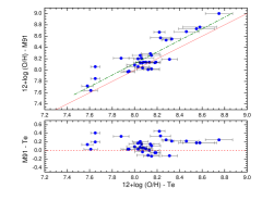
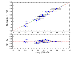
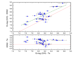
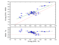
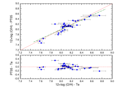
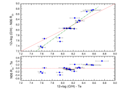
Figure 2: Comparison between the oxygen abundances derived using the direct method ($T_{\rm e}$, always plotted in the $x-axis$) with those estimated using six different empirical calibrations that consider the $R_{23}$ parameter: M91: McGaugh (1991); P01: Pilyugin (2001a, b); KD02: Kewley & Dopita (2002); KK04: Kobulnicky & Kewley (2004); PT05: Pilyugin & Thuan (2005); N06: Nagao et al. (2006). The bottom panel of each diagram indicates the difference between empirical and direct data.

We used the data of the 31 regions for which we have a direct estimate of $T_{\rm e}$ and, hence, a direct estimate of the oxygen abundance –see López-Sánchez & Esteban (2010b) and their Table 3– , to check the reliability of several empirical calibrations. A recent review of 10 metallicity calibrations, including theoretical and empirical methods, was presented by Kewley & Ellison (2008), but previous section gives an overview of the most common empirical calibrations and defines the typical parameters that are used to estimate the oxygen abundance following these relations. These parameters are ratios between bright emission lines, the most commonly used are $R_{23}$, $P$, $y$, $N_{2}$, and $O_{3}N_{2}$ Table 1 lists the values of all these parameters derived for each region with a direct estimate of the oxygen abundance –see López-Sánchez & Esteban (2009) for details–. Table 1 also includes the value derived for the $q$ parameter (in units of cm s^-1) obtained from the optimal calibration provided by Kewley & Dopita (2002). The results for the oxygen abundances derived for each object and empirical calibration are listed in Table 2. This table also indicates the branch (high or low metallicity) considered in each region when using the $R_{23}$ parameter although, as is clearly specified in the table, for some objects with 8.00$\leq$12+log(O/H)$\leq$8.3 we assumed the average value found for the lower and upper branches.

Looking at the data compiled in Table 2 the huge range of oxygen abundance found for the same object using different calibrations is evident. As Kewley & Ellison (2008) concluded, it is critical to use the same metallicity calibration when comparing properties from different data sets or investigate luminosity-metallicity or mass-metallicity relations. Furthermore, abundances derived with such strong-line methods may be significantly biased if the objects under study have different structural properties (hardness of the ionizing radiation field, morphology of the nebulae) than those used to calibrate the methods (Stasińska, 2009).

Figures 2 and 3 plots the ten most common calibrations and their comparison with the oxygen abundance obtained using the direct method. We performed a simple statistic analysis of the results to quantify the goodness of these empirical calibrations. Table 3 compiles the average value and the dispersion (in absolute values) of the difference between the abundance given by empirical calibration and that obtained using the direct method. We check that the empirical calibration that provides the best results is that proposed by Pilyugin (2001a, b), which gives oxygen abundances very close to the direct values (the differences are lower than 0.1 dex in the majority of the objects), and furthermore it possesses a low dispersion. We note however that the largest divergences found using this calibration are in the low-metallicity regime. The update of this calibration presented by Pilyugin & Thuan (2005) seems to partially solve this problem, the abundances provided by this calibration also agree very well with those derived following the direct method. We therefore conclude that the Pilyugin & Thuan (2005) calibration is nowadays the best suitable method to derive the oxygen abundance of star-forming galaxies when auroral lines are not observed.

On the other hand, the results given by the empirical calibrations provided by McGaugh (1991), Kewley & Dopita (2002) and Kobulnicky & Kewley (2004), that are based on photoionization models, are systematically higher than the values derived from the direct method. This effect is even more marked in the last two calibrations, which usually are between 0.2 and 0.3 dex higher than the expected values. These empirical calibrations also have a higher dispersion than that estimated for Pilyugin (2001a, b) or Pilyugin & Thuan (2005) calibrations. Yin et al (2007) also found high discrepancies when comparing the theoretical metallicities using the theoretical models of Tremonti et al. (2004) with the $T_{\rm e}$-based metallicites obtained from Pilyugin (2001a, b) and Pilyugin & Thuan (2005).

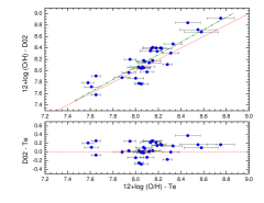
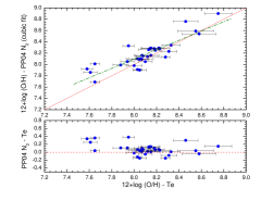
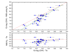
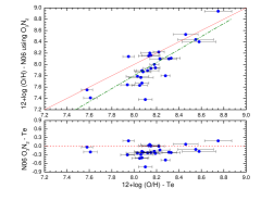
Figure 3: Comparison between the oxygen abundances derived using the direct method ($T_{\rm e}$, in the $x-axis$) with those computed using the calibrations using the $N_{2}$ parameter –D02: Denicoló, Terlevich & Terlevich (2002); PP04b: Pettini & Pagel (2004) considering their cubic fit to $N_{2}$; N06: Nagao et al. (2006)– and the O₃N₂ parameter following the cubic fit provided by Nagao et al. (2006). The bottom panel of each diagram indicates the difference between empirical and direct data.

One of the possible explanations for the different metallicities obtained between the direct method and those derived from the empirical calibrations based on photoionization models are temperature fluctuations in the ionized gas. Temperature gradients or fluctuations indeed cause the true metallicities based on the $T_{\rm e}$-method to be underestimated (i.e. Peimbert 1967; Stasinska 2002,2005; Peimbert et al. 2007). Temperature fluctuations can also explain our results for NGC 5253 (López-Sánchez et al., 2007): the ionic abundances of O⁺⁺/H⁺ and C⁺⁺/H⁺ derived from recombination lines are systematically 0.2 – 0.3 dex higher than those determined from the direct method –based on the intensity ratios of collisionally excited lines. This abundance discrepancy has been also found in Galactic (García-Rojas & Esteban, 2007) and other extragalactic (Esteban et al., 2009) H ii regions and interestingly this discrepancy is in all cases of the same order as the differences between abundances derived from the direct methods and empirical calibrations based on photoionization models.

The conclusion that temperature fluctuations do exist in the ionized gas of starburst galaxies is very important for the analysis of the chemical evolution of galaxies and the Universe. Indeed, if that is correct, the majority of the abundance determinations in extragalactic objects following the direct method, including those provided in this work, have been underestimated by at least 0.2 to 0.3 dex. Deeper observations of a large sample of star-forming galaxies –that allow us to detect the faint recombination lines, such as those provided by Esteban et al. (2009)– and more theoretical work –including a better understanding of the photoionization models, such as the analysis provided by Kewley & Ellison (2008)– are needed to confirm this puzzling result.

Table 3: Results of the comparison between the oxygen abundance given by several empirical calibrations and the oxygen abundance derived here following the direct ($T_{\rm e}$) method.

Parameter	$R_{23}$							$N_{2}$				$O_{3}N_{2}$
Calibrationa	P01	PT05	N06	M91	KD02	KK04		D02	PP04	N06		PP04	N06
Averageb	0.07	0.08	0.14	0.15	0.28	0.27		0.14	0.12	0.18		0.12	0.21
$\sigma^{c}$	0.05	0.07	0.12	0.11	0.18	0.13		0.10	0.10	0.14		0.10	0.16
Notesd	B/A (1)	B/A	(2)	S.H.	S.H.	S.H.		S.H. (3)	B/A (4)	S.L.(5)		B/A (6)	S.L.

^a The names of the calibrations are the same as in Table 2.

^b Average value (in absolute values) of the difference between the abundance given by empirical calibrations and that obtained using the direct method. The names of the calibrations are the same as in Table 2.

^c Dispersion (in absolute values) of the difference between the abundance given by empirical calibrations and that obtained using the direct method.

$d$ We indicate if the empirical calibration gives results both below and above the direct value (B/A), if they are systematically higher than the direct value (S.H.) or if they are systematically lower than the direct value (S.L.). Some additional notes are:

(1) Higher deviation in the low branch.

(2) This calibration provides lower oxygen abundances in low-metallicity regions and higher oxygen abundances in high-metallicity regions.

(3) Systematically higher only for 12+log(O/H)$>$8.2.

(4) Higher deviation for 12+log(O/H)$<$8.0. Considering 12+log(O/H)$>$8.0, we get average=0.08 and $\sigma$=0.06.

(5) Higher deviation at lower oxygen abundances.

(6) Higher deviation for 12+log(O/H)$<$8.0. Assuming 12+log(O/H)$>$8.0, average=0.09 and $\sigma$=0.06.

On the other hand, we have checked the validity of the recent relation provided by Nagao et al. (2006), which merely considers a cubic fit between the $R_{23}$ parameter and the oxygen abundance. This calibration was obtained combining data from several large galaxy samples, the majority from the SDSS, which includes all kinds of star-forming objects. As it is clearly seen in Table 2 and in Fig. 3, the Nagao et al. (2006) relation is not suitable to derive a proper estimate of the oxygen abundance for the majority of the objects in our galaxy sample. In general, this calibration provides lower oxygen abundances in low-metallicity regions and higher oxygen abundances in high-metallicity regions. Objects located in the metallicity range 8.00$\leq$12+log(O/H)$\leq$8.15 have systematically 12+log(O/H)${}_{\rm N06}\sim$8.07 because we have to use an average value between the low and the high branches. Furthermore, many of the regions do not have a formal solution to the Nagao et al. (2006) equation, such as the maximum value for $R_{23}$ is 8.39 at 12+log(O/H)=8.07. We consider that the use of an ionization parameter –$P$ as introduced by Pilyugin (2001a, b) or $q$ as followed by Kewley & Dopita (2002)– is fundamental to obtain a real estimate of the oxygen abundance in star-forming galaxies, especially in objects showing strong starbursts. In the same sense, the direct method and not the formulae provided by Izotov et al. (2006) (which assumes a low-density approximation in order not to have to solve the statistical equilibrium equations of the O⁺² ion) provides a good approximation to the actual oxygen abundance when the auroral line [O iii] $\lambda$4653 is observed.

Empirical calibrations considering a linear fit to the $N_{2}$ ratio (Denicoló, Terlevich & Terlevich, 2002; Pettini & Pagel, 2004) give results that are systematically $\sim$0.15 dex higher that the oxygen abundances derived from the direct method. The difference is higher at higher metallicities. We do not consider that this trend is a consequence of comparing different objects: both Denicoló et al. (2002) and Pettini & Pagel (2004) calibrations are obtained using a sample of star-forming galaxies similar to those analysed in this work, many of which are WR galaxies. Denicoló et al. (2002) compared the $N_{2}$ ratio with the ionization parameter together with the results of photoionization models and concluded that most of the observed trend of $N_{2}$ with the oxygen abundance is caused by metallicity changes. The cubic fit to $N_{2}$ performed by Pettini & Pagel (2004) better reproduces the oxygen abundance, especially in the intermediate- and high-metallicity regime (12+log(O/H)$>$8.0), where it has an average error of $\sim$0.08 dex. However, the cubic fit to $N_{2}$ provided by Nagao et al. (2006) gives systematically lower values for the oxygen abundance than those derived using the direct method, having an average error of $\sim$0.18 dex.

The empirical calibration between the oxygen abundance and the $O_{3}N_{2}$ parameter proposed by Pettini & Pagel (2004) gives acceptable results for objects with 12+log(O/H)$>$8.0, with the average error $\sim$0.1 dex. However, the new relation provided by Nagao et al. (2006) involving the $O_{3}N_{2}$ parameter gives systematically lower values for the oxygen abundance. As we commented before, we consider that the Nagao et al. (2006) calibrations are not suitable for studying galaxies with strong star-formation bursts. Their procedures must be taken with caution, galaxies with different ionization parameters, different chemical evolution histories, and different star formation histories should have different relations between the bright emission lines and the oxygen abundance. This issue is even more important when estimating the metallicities of intermediate- and high-redshift galaxies, because the majority of their properties are highly unknown.

4 Conclusions

We compared the abundances provided by the direct method with those obtained using the most common empirical calibrations in our sample of star-forming regions within Wolf-Rayet galaxies –see López-Sánchez & Esteban (2010b)–. The main conclusions are:

• The Pilyugin-method of Pilyugin (2001a, b), which considers the $R_{23}$ and the $P$ parameters and is updated by Pilyugin & Thuan (2005), is nowadays the best suitable empirical calibration to derive the oxygen abundance of star-forming galaxies. The cubic fit to $R_{23}$ provided by Nagao et al. (2006) is not valid for analysing these star-forming galaxies.

• The relations between the oxygen abundance and the $N_{2}$ or the $O_{3}N_{2}$ parameters provided by Pettini & Pagel (2004) give acceptable results for objects with 12+log(O/H)$>$8.0.

• The results provided by empirical calibrations based on photoionization models (McGaugh, 1991; Kewley & Dopita, 2002; Kobulnicky & Kewley, 2004) are systematically 0.2 – 0.3 dex higher than the values derived from the direct method. These differences are of the same order as the abundance discrepancy found between abundances determined from recombination and collisionally excited lines of heavy-element ions. This may suggest temperature fluctuations in the ionized gas, as they exist in Galactic and other extragalactic H ii  regions.

- (1)
- Alloin et al. (1979) Alloin D., Collin-Souffrin S., Joly M. & Vigroux L. 1979, A&A, 78, 200
- Crowther (2007) Crowther, P.A. 2007, ARAA, 45, 177
- Denicoló, Terlevich & Terlevich (2002) Denicoló, G., Terlevich, R. & Terlevich, E. 2002, MNRAS, 330, 69
- de Naray, McGaugh & de Blok (2004) de Naray R. K., McGaugh S. S. & de Blok W. J. G., 2004, MNRAS, 355, 887
- De Rossi et al. (2006) De Rossi, M.E., Tissera, P.B., & Scannapieco, C. 2006, MNRAS, 374, 323
- Díaz & Pérez-Montero (2000) Díaz, A.I., & Pérez-Montero, E. 2000, MNRAS, 312, 130
- Dopita & Evans (1986) Dopita, M.A. & Evans, I. N. 1986, ApJ, 307, 431
- Dopita et al. (2000) Dopita, M.A., Kewley, L. J., Heisler, C.A. & Sutherland, R.S. 2000, ApJ, 542, 224
- Edmunds & Pagel (1978) Edmunds, M.G. & Pagel, B.E.J. 1978, MNRAS, 185, 77
- Edmunds & Pagel (1984) Edmunds, M.G. & Pagel, B.E.J. 1984, MNRAS, 211, 507
- Erb et al. (2006) Erb, D.K., Shapley, A.E., Pettini, M., Steidel, C.C., Reddy, N.A. & Adelberger, K.L. 2006, ApJ, 644, 813
- Esteban et al. (2009) Esteban, C., Bresolin, F., Peimbert, M., García-Rojas, J., Peimbert, A. & Mesa-Delgado, A. 2009, ApJ, 700, 654
- Ferland et al. (1998) Ferland G. J., Korista K. T., Verner D. A., Ferguson J. W., Kingdon J. B. & Verner E. M, 1998, PASP, 110, 761
- Fioc & Rocca-Volmerange (1997) Fioc, M. & Rocca-Volmerange, B. 1997, A&A 326, 950
- García-Rojas & Esteban (2007) García-Rojas, J. & Esteban, C., 2007, ApJ, 670, 457
- Garnett (1992) Garnett, D.R. 1992, AJ, 103, 1330
- Hirashita et al. (2001) Hirashita, H., Inoue, A.K., Kamaya, H. & Shibai, H. 2001, A&A, 366, 83
- Izotov et al. (2006) Izotov, Y.I., Stasińska, G., Meynet, G., Guseva, N.G. & Thuan, T.X. 2006, A&A, 448, 955
- Jensen, Strom & Strom (1976) Jensen E. B., Strom K. M. & Strom S. E. 1976, ApJ, 209, 748
- Kewley et al. (2001) Kewley, L.J., Dopita, M.A., Sutherland, R.S., Heisler, C.A. & Trevena, J. 2001, ApJS, 556, 121
- Kewley & Dopita (2002) Kewley, L.J. & Dopita, M.A. 2002, ApJS, 142, 35
- Kewley & Ellison (2008) Kewley, L.J., & Ellison, S.E. 2008, ApJ, 681, 1183
- Kobulnicky, Kennicutt & Pizagno (1999) Kobulnicky, H.A, Kennicutt, R.C.Jr. & Pizagno, J.L. 1999, ApJ 514, 544
- Kobulnicky & Kewley (2004) Kobulnicky H. A. & Kewley L. J. 2004, ApJ, 617, 240
- Kobulnicky et al. (2003) Kobulnicky, H. A., Willmer, C.N.A., Phillips, A.C., Koo, D.C., Faber, S.M., Weiner, B.J., Sarajedini, V.L., Simard, L. & Vogt, N.P. 2003, ApJ 599, 1006
- Leitherer et al. (1999) Leitherer, C., Schaerer, D., Goldader, J.D., González-Delgado, R.M., Robert, C., Kune, D.F., de Mello, D.F., Devost, D. & Heckman, T.M. 1999, ApJS, 123, 3 (STARBURST 99)
- Lilly et al. (2003) Lilly, S.J., Carollo, C.M. & Stockton, A.N. 2003, ApJ, 597, 730
- López-Sánchez (2006) López-Sánchez, Á.R. 2006, PhD Thesis, Universidad de la Laguna (Tenerife, Spain)
- López-Sánchez, Esteban & Rodríguez (2004a) López-Sánchez, Á.R., Esteban, C. & Rodríguez, M. 2004a, ApJS, 153, 243
- López-Sánchez, Esteban & Rodríguez (2004b) López-Sánchez, Á.R., Esteban, C. & Rodríguez, M. 2004b, A&A, 428, 445
- López-Sánchez, Esteban & García-Rojas (2006) López-Sánchez, Á.R., Esteban, C. & García-Rojas, J. 2006, A&A, 449, 997
- López-Sánchez et al. (2007) López-Sánchez, Á.R., Esteban, C., García-Rojas, J., Peimbert, M. & Rodríguez, M. 2007, ApJ, 656, 168
- López-Sánchez & Esteban (2008) López-Sánchez, Á.R. & Esteban, C. 2008, A&A, 491, 131, Paper I
- López-Sánchez & Esteban (2009) López-Sánchez, Á.R. & Esteban, C. 2009, A&A, 508, 615, Paper II
- López-Sánchez & Esteban (2010a) López-Sánchez, Á.R. & Esteban, C. 2010a, A&A, in press, Paper III
- López-Sánchez & Esteban (2010b) López-Sánchez, Á.R. & Esteban, C. 2010,b A&A, in press, Paper IV
- López-Sánchez et al. (2010) López-Sánchez, Á.R. et al. 2010, A&A, in revision, Paper V
- McCall, Rybski & Shields, (1985) McCall, M.L., Rybski, P.M. & Shields, G.A. 1985, ApJS 57, 1
- McGaugh (1991) McGaugh, S.S. 1991, ApJ, 380, 140
- Nagao, Maiolino & Marconi (2006) Nagao, T., Maiolino, R. & Marconi, A. 2006, A&A, 459, 85
- Oey & Shields (2000) Oey M. S. % Shields J. C., 2000, ApJ, 539, 687
- Pagel et al. (1979) Pagel, B. E. J., Edmunds, M. G., Blackwell, D. E., Chun, M. S., Smith, G. 1979, MNRAS, 189, 95
- Peimbert (1967) Peimbert, M. 1967, ApJ, 150, 825
- Peimbert et al. (2007) Peimbert, M., Peimbert, A.. Esteban, C.; García-Rojas, J., Bresolin, F., Carigi, L., Ruiz, M.T. & López-Sánchez, Á.R. 2007, RMxAC, 29, 72
- Pérez-Montero & Díaz (2005) Pérez-Montero, E. & Díaz, A. I. 2005, MNRAS, 361, 1063
- Pettini & Pagel (2004) Pettini, M. & Pagel, B.E.J. 2004, MNRAS, 348, 59
- Pilyugin (2000) Pilyugin, L.S. 2000, A&A, 362, 325
- Pilyugin (2001a) Pilyugin, L.S. 2001a, A&A, 369, 594
- Pilyugin (2001b) Pilyugin, L.S. 2001b, A&A, 374, 412
- Pilyugin, Vílchez & Contini (2004) Pilyugin, L. S., Vílchez, J. M. & Contini, T. 2004, A&A, 425, 849
- Pilyugin & Thuan (2005) Pilyugin, L.S. & Thuan, T.X. 2005, ApJ, 631, 231
- Schaerer, Contini & Pindao (1999) Schaerer, D., Contini, T. & Pindao, M. 1999, A&AS 136, 35
- Stasińska (2002) Stasińska, G. 2002, RMxAC, 12, 62
- Stasińska (2005) Stasińska, G. 2005, A&A, 434, 507
- Stasińska (2006) Stasińska, G. 2006, A&A, 454, 127
- Stasińska (2009) Stasińska, G. 2009, proceedings of IAU sumposium 262, Stellar Populations - planning for the next decade, eds Bruzual & Charlot, astro-ph:0910.0175
- Storchi-Bergmann, Calzetti & Kinney (1994) Storchi-Bergmann, T., Calzetti, D. & Kinney, A.L. 1994, ApJ, 429, 572
- Sutherland & Dopita (1993) Sutherland, R.S. & Dopita, M.A. 1993, ApJS, 88, 253
- Teplitz et al. (2000) Teplitz, H.I., Malkan, M.A., Steidel, C.C., McLean, I.S., Becklin, E.E., Figer, D.F., Gilbert, A.M., Graham, J.R., Larkin, J.E., Levenson, N.A. & Wilcox, M.K. 2000, ApJ, 542, 18
- Torres-Peimbert et al. (1989) Torres-Peimbert, S., Peimbert, M. & Fierro, J. 1989, ApJ, 345, 186
- Tremonti et al. (2004) Tremonti, C.A., et al. 2004, ApJ, 613, 898
- van Zee, Salzer & Haynes (1998) van Zee, L., Salzer, J.J. & Haynes, M.P. 1998, ApJ, 497, 1
- Vázquez & Leitherer (2005) Vázquez, G.A. & Leitherer, C. 2005, ApJ, 621, 695
- Vila-Costas & Edmunds (1992) Vila-Costas, M. B. & Edmunds, M. G. 1993, MNRAS, 259, 121
- Vila-Costas & Edmunds (1993) Vila-Costas, M. B. & Edmunds, M. G. 1993, MNRAS, 265, 199
- Vílchez & Esteban (1996) Vílchez, J.M., & Esteban, C. 1996, MNRAS, 280, 720
- Woosley & Weaver (1995) Woosley S. E. & Weaver, T.A. 1995, ApJS, 101, 181
- Yin et al (2007) Yin, S.Y., Liang, Y.C., Hammer, F., Brinchmann, J., Zhang, B., Deng, L.C. & Flores, H., 2007, A&A, 462, 535
- York et al. (2000) York, D.G. et al. 2000, AJ, 120, 1579
- Zaritsky, Kennicutt & Huchra (1994) Zaritsky, D., Kennicutt, R. C. Jr. & Huchra, J.P. 1994, ApJ 420, 87
- (72)