Robustness maximization of parallel multichannel systems

Abstract

Bit error rate (BER) minimization and SNR-gap maximization, two robustness optimization problems, are solved, under average power and bit-rate constraints, according to the waterfilling policy. Under peak-power constraint the solutions differ and this paper gives bit-loading solutions of both robustness optimization problems over independent parallel channels. The study is based on analytical approach with generalized Lagrangian relaxation tool and on greedy-type algorithm approach. Tight BER expressions are used for square and rectangular quadrature amplitude modulations. Integer bit solution of analytical continuous bit-rates is performed with a new generalized secant method. The asymptotic convergence of both robustness optimizations is proved for both analytical and algorithmic approaches. We also prove that, in conventional margin maximization problem, the equivalence between SNR-gap maximization and power minimization does not hold with peak-power limitation. Based on a defined dissimilarity measure, bit-loading solutions are compared over power line communication channel for multicarrier systems. Simulation results confirm the asymptotic convergence of both allocation policies. In non asymptotic regime the allocation policies can be interchanged depending on the robustness measure and the operating point of the communication system. The low computational effort of the suboptimal solution based on analytical approach leads to a good trade-off between performance and complexity.

I Introduction

In transmitter design, a problem often encountered is resource allocation among multiple independent parallel channels. The resource can be the power, the bits or the data and the number of channels. The allocation policies are performed under constraints and assumptions, and the independent parallel channels can be encountered in multitone transmission or multiantenna communications.

Independent parallel channels result from orthogonal design applied in time, frequency or spatial domains [1]. They can either be obtained naturally or in a situation where the transmit and receive strategies are to orthogonalize multiple waveforms. Orthogonal frequency-division multiplexing (OFDM) and digital multitone (DMT) are two successful commercial applications for wireless and wireline communications with orthogonality in the frequency domain. In multiantenna communications, the parallel channels are made from the singular vectors of the multiple-input multiple-output (MIMO) channel [2]. This MIMO concept and the resulting orthogonal design can be applied in many communication scenarios when there are multiple transmit and receive dimensions [3].

To perform allocation, mathematical relations between various resources are needed and the first one is the channel capacity. This capacity of $n$ independent parallel Gaussian channels is the well-known sum of the capacities of each channel

$$\mathcal{C}=\sum_{i=1}^{n}\mathcal{C}_{i}=\sum_{i=1}^{n}\log_{2}(1+\mathsf{snr}_{i})\,.$$ (1)

This relation, which holds for memoryless channels, links the supremum bit-rate $\mathcal{C}_{i}$, here expressed in bit per two dimensions, to the signal to noise ratio, $\mathsf{snr}_{i}$, experienced by each channel or subchannel $i$. Any reliable and implementable system must transmit at a bit-rate $r_{i}$ below capacity $\mathcal{C}_{i}$ over each subchannel and then the margin, or SNR-gap, $\gamma_{i}$ is introduced to analyze such systems [4, 5]

$$\gamma_{i}=\frac{2^{\mathcal{C}_{i}}-1}{2^{r_{i}}-1}\,.$$ (2)

This SNR-gap is a convenient mechanism for analyzing systems that transmit below capacity, and

$$r_{i}=\log_{2}\Big{(}1+\frac{\mathsf{snr}_{i}}{\gamma_{i}}\Big{)},$$ (3)

with $r_{i}$ the bit-rate in bits per two dimensional-symbol (bits per second per subchannel) which is also the number of bits per constellation symbol.

Resource allocation is performed using loading algorithms and diverse criteria can be invoked to decide which portion of the available resource is allocated to each of the subchannels. From information theory point of view, the criterion is the mutual information and the optimal allocation under average power constraint was first devised in [6] for Gaussian inputs and later for non-Gaussian inputs [7]. Since the performance measure is the mutual information in these cases, the SNR-gap in (3) is $\{\gamma_{i}\}_{i=1}^{n}=1$. In other cases, $\{\gamma_{i}\}_{i=1}^{n}>1$ and (3), as enhanced relationships, leads to many optimal and suboptimal allocation policies. In fact, resource allocation is a constraint optimization problem and generally two cases are of practical interest: rate maximization (RM) and margin maximization (MM), where the objective is the maximization of the data or bit-rate, and the maximization of the system margin (or power minimization in practice), respectively [8]. The MM problem gathers all non RM problems including power minimization, margin maximization (in its strict sense) and other measures such as error probabilities or goodput. Among all the resource allocation strategies, equivalence or duality can be found defining family of approaches and using unified processes [9, 10, 11, 12]. The loading algorithms are also split in two families. The first is based on greedy-type approach to iteratively distribute the discrete resources [13], and the second uses Lagrangian relaxation to solve continuous resource adaptation [14]. Both approaches have been compared in terms of performance and complexity [15, 14, 9, 16]. All these adaptive resource allocations are possible when channel state information (CSI) is known at both transmitter and receiver sides. This CSI can be perfect or imperfect, and full or partial. The effects of channel estimation error and feedback delay on the performance of adaptive modulated systems can also be considered in the allocation process [17, 18, 19].

In this paper we shall focus henceforth on MM problems with perfect and full CSI consideration, and under peak-power and bit-rate constraints. It is assumed that the channel estimation is perfect, and feedback CSI delay and overhead are negligible. Peak-power constraint results from power mask limitation and has been taken into account in resource allocation problem [15, 20, 21, 22] instead of the conventional average power constraint, or sum power constraint, which is historically the first considered constraint [6]. Bit-rate constraint comes from communication applications or service requirements, where different flows can exist but one of them is chosen at the beginning of the communication. In this configuration, the remaining parameter to optimize is then the SNR-gap $\gamma_{i}$ which is also related to the error probability of the communication system.

Two similar problems of MM have the same objective that is to maximize the system robustness. What we call robustness in this paper is the capability of a system to maintain acceptable performance with unforeseen disturbances.

The first measure of robustness is the SNR-gap, or system margin, and its maximization ensures protection to unforeseen channel impairments or noise. The system margin maximization is the maximization of the minimal SNR-gap $\gamma_{i}$ in (3) over the $n$ subchannels. In that case the conventional equivalence between margin maximization and power minimization in MM problems is not generally true. In this paper we show that this equivalence can nevertheless be obtained in particular configurations.

The second robustness measure is the bit error rate (BER) and its minimization can reduce the packet error rate and the data retransmission. In transmitter design, the BER minimization can be realized using uniform bit-loading and adaptive precoding [23, 24]. Analytical studies have been performed with peak-BER or average BER (computed as arithmetic mean) approaches [17, 19]. With average BER computed as weighted arithmetic mean, the resource allocation has been performed using greedy-type algorithm [25]. The first main contribution in this paper is the analytical solution of the resource allocation problem in the case of weighted arithmetic mean BER minimization.

To perform the analytical study based on generalized Lagrangian relaxation tool, we develop a new method for finding roots of functions. This method generalizes the secant method to better fit the function-depending weight and to speed up the search of the roots. Both robustness polices are compared with a new measure that evaluates the difference in the bit distribution between two allocations. We also prove that both robustness policies provide the same bit distribution in asymptotic regime and this is the second main contribution in this paper. The proof is given in the case of unconstrained modulations (i.e. continuous bit-rates and analytical solution) and also for QAM constellations and greedy-type algorithms. The convergence is exemplified by simulation in multicarrier PLC (power line communications) systems.

The organization of the paper is as follows. In Section II, the quantities to be used throughout the paper are introduced and the robustness optimization problem is formulated in a general way for both system margin maximization and BER minimization. The cases of equivalence between margin maximization and power minimization are worked out. Section III is an interlude, presenting the considered expressions of accurate BER, a new measure of allocation differences and a new search method of root function. The solution of formulated problems are given in Section IV in the form of an optimum allocation policy based on greedy-type algorithms. The conditions of equivalence of both margin maximization and BER minimization are given in this section. Section V presents the analytical solution and both greedy-type and analytical methods are compared in Section VI. In turn, Section VII exemplifies the application of robustness optimization to multicarrier PLC systems. Finally, the paper concludes in Section VIII with the proofs of several results relegated to the appendices.

Notation. The bit-rates $\{r_{i}\}_{i=1}^{n}$ are defined as a number of bits per two dimensions and they also could only be a number of bits (undertone per constellation). Without confusing, the unit of the variable $r_{i}$ are not all the time fully expressed.

II Problem formulation

Consider $n$ parallel subchannels. On the $i$th subchannel, the input-output relationship is

$$Y_{i}=h_{i}S_{i}+W_{i}\ ,$$ (4)

with $S_{i}$ the transmitted symbol, $Y_{i}$ the received one, and $h_{i}$ the complex scalar channel gain. The complex Gaussian noise $W_{i}$ is a proper complex random variable with zero-mean and variance equal to $\sigma_{W_{i}}^{2}$.

The conventional average power constraint is

$$\frac{1}{n}\sum_{i=1}^{n}E[|S_{i}|^{2}]\leq P\ ,$$ (5)

whereas the peak-power constraint, or power spectrum density constraint, considered in this paper is

$$\forall i\in[1,n]\quad E[|S_{i}|^{2}]\leq P\,.$$ (6)

It is convenient to use normalized unit-power symbol $\{X_{i}\}_{i=1}^{n}$ such that

$$S_{i}=\sqrt{p_{i}P}X_{i}\,,$$ (7)

which leads to the peak-power constraint

$$\forall i\in[1,n]\quad p_{i}\leq 1\,.$$ (8)

It is also convenient to introduce two other variables. The first one is the conventional SNR

$$\mathsf{snr}_{i}=|h_{i}|^{2}p_{i}\frac{P}{\sigma_{W_{i}}^{2}}$$ (9)

and the second is called power spectrum density noise ratio (PSDNR)

$$\mathsf{psdnr}=\frac{1}{n}\sum_{i=1}^{n}|h_{i}|^{2}\frac{P}{\sigma_{W_{i}}^{2}}\,,$$ (10)

which is the mean signal to noise ratio over the $n$ subchannels if and only if $\forall i$ $p_{i}=1$. This PSDNR is the ratio between the power mask at receiver side (the transmitted power mask through the channel) and the power spectrum density of the noise. The system performance will be given according to this parameter to point out the ability of a system to exploit the available power under peak-power constraint.

Using the previous notations, (3) becomes

$$r_{i}= \log_{2}\Big{(}1+\frac{|h_{i}|^{2}p_{i}P}{\gamma_{i}\sigma_{W_{i}}^{2}}\Big{)}\,.$$ (11)

With $p_{i}/\gamma_{i}=1$ for all $i$, $r_{i}$ is the subchannel capacity under power constraint $P$. With unconstrained modulations, $r_{i}$ is defined in $\mathbb{R}$, but constrained modulations are used in practice and $r_{i}$ takes a finite number of nonnegative values. Non integer number of bits per symbol can also be used with fractional bit constellations [26, 27]. In this paper, modulations defined by discrete points are used with integer number of bits per symbol. Typically, $r_{i}\in\{0{,}\beta{,}2\beta{,}\cdots{,}r_{\text{max}}\}$, where $\beta$ is the granularity in bits and $r_{\text{max}}$ is the number of bits in the richest available constellation. When all QAM constellations are used $\beta=1$. The peak-power and bit-rate constraints are then

$$\forall i\ p_{i}\leq 1,\ \displaystyle\sum_{i=1}^{n}r_{i}=R,\ \forall i\ r_{i}\in\{0{,}\beta{,}2\beta{,}\cdots{,}r_{\text{max}}\}\,.$$ (12)

Obviously, the exploitation of available power leads to $\forall i\ p_{i}=1$ and the constraint is simplified

$$\displaystyle\sum_{i=1}^{n}r_{i}=R,\quad\forall i\ r_{i}\in\{0{,}\beta{,}2\beta{,}\cdots{,}r_{\text{max}}\}\,.$$ (13)

With peak-power and bit-rate constraints, the allocation strategy is then to use all available power and to optimize the robustness.

The problem we pose is to determine the optimal bit-rate allocation $\{r_{i}^{*}\}_{i=1}^{n}$ that maximizes a robustness measure, or inversely minimizes a frailness measure, with given SNR of subchannels while satisfying (13). In its general form, this problem can be written as

$$[r_{1}^{*},\cdots,r_{n}^{*}]=\arg\min_{\eqref{eq_const}}\phi\Big{(}\{r_{i}\}_{i=1}^{n}\Big{)},$$ (14)

where $\phi(\cdot)$ is the frailness measure. In this paper, this measure is given by the SNR-gap or the BER. In addition to the bit-rate allocation, the receiver is presumed to have knowledge of the magnitude and phase of the channel gain $\{h_{i}\}_{i=1}^{n}$, whereas the transmitter needs only to know the magnitude $\{|h_{i}|\}_{i=1}^{n}$. The objective is to find the data vector $[r_{1}^{*},\cdots,r_{n}^{*}]$ which is the final relevant information for the transmitter. The allocation can then be computed on the receiver side to reduce the feedback data-rate from $n$ real numbers to $n$ finite integer numbers. Furthermore, the integer nature of the data-rates allows a full CSI at the transmitter which is not possible with real numbers.

II-A System margin maximization

The SNR-gap $\gamma_{i}$ of the subchannel $i$ is (3)

$$\gamma_{i}=\frac{\mathsf{snr}_{i}}{2^{r_{i}}-1}\,.$$ (15)

With reliable communications, $\gamma_{i}$ is higher than 1 for all subchannels. Let the system margin, or system SNR-gap, be the minimal value of the SNR-gap in each subchannel

$$\gamma=\min_{i}\gamma_{i}\,.$$ (16)

Let $\gamma_{\text{init}}$ be the initial system margin of one communication system ensuring a given QoS. Let $\gamma$ be the optimized system margin of this system. Then, the system margin improvement ensure system protection in unforeseen channel impairment or noise, e.g. impulse noise: bit-rate and system performance targets are always reached for an unforeseen SNR reduction of $\gamma/\gamma_{\text{init}}$ over all subchannels. This robustness optimization does not depend on constellation and channel coding types. The system margin $\gamma$ is defined and optimized without knowledge of used constellations and coding, and the proposed robustness optimization works for any coding and modulation scheme.

The objective is the maximization of the system margin which is equivalent to the minimization of $\gamma^{-1}$. We note $\gamma_{i}(r_{i})$ the function that associates $r_{i}$ to $\gamma_{i}$. The function $\phi(\cdot)$ in (14) is then given by

$$\phi\Big{(}\{r_{i}\}_{i=1}^{n}\Big{)}=\max_{i}\frac{1}{\gamma_{i}(r_{i})}$$ (17)

and

$$[r_{1}^{*}{,}\cdots{,}r_{n}^{*}]=\arg\min_{\eqref{eq_const}}\max_{i}\gamma_{i}^{-1}\,.$$ (18)

This problem is the converse problem of bit-rate maximization under peak-power and SNR-gap constraints. The solution of the bit-rate maximization problem is obvious under the said constraints and given by

$$\forall i\quad r_{i}^{*}=\beta\left\lfloor\frac{1}{\beta}\log_{2}\left(1+\frac{\mathsf{snr}_{i}}{\gamma_{i}}\right)\right\rfloor.$$ (19)

Following the conventional SNR-gap approximation [4], symbol error rate (SER) expression of QAM depending on SNR-gap is constellation size-independent with

$$\forall r_{i}\quad\mathsf{ser}_{i}(r_{i})=2\operatorname{erfc}\left(\sqrt{\frac{3}{2}\gamma_{i}}\right)\,,$$ (20)

where the complementary error function is usually defined as

$$\operatorname{erfc}\left(x\right)=\frac{2}{\sqrt{\pi}}\int_{x}^{\infty}e^{-t^{2}}\operatorname{d}\!t\,.$$ (21)

The system margin maximization is then equivalent to the peak-SER minimization in high SNR regime. Note that with (16), the system margin maximization can also be called a trough-SNR-gap maximization and it strongly related to the peak-power minimization. Whereas the bit-loading solution is the same for power minimization and margin maximization, with sum-margin or sum-power constraints instead of peak constraints, the following lemma gives sufficient conditions for equivalence in the case of peak constraints.

Lemma 1

The bit allocation, that maximizes the system margin under peak-power constraint $\{p_{i}^{\text{margin}}\}_{i=1}^{n}$, minimizes the peak-power under SNR-gap constraint $\{\gamma_{i}^{\text{power}}\}_{i=1}^{n}$ if $p_{i}^{\text{margin}}\gamma_{i}^{\text{power}}=\alpha$ for all $i$.

Proof:

It is straightforward using (11) and (18). Both problems have the same expression and therefore the same solution. ∎

This lemma provides a sufficient but not necessary condition for the equivalence of solutions, and it says that if the power and the SNR-gap constraints have proportional distributions for margin maximization and peak-power minimization problems, respectively, then both problems have the same optimal bit-rate allocation. This lemma also shows that both problems don’t have the same solution in a general case. A particular case is the uniform distribution of $\{p_{i}\}_{i=1}^{n}$ which is the case analyzed in this paper.

II-B BER minimization

In communication systems, the error rate of the transmitted bits is a conventional robustness measure. By definition, the BER is the ratio between the number of wrong bits and the number of transmitted bits. With a multidimensional system, there exists several BER expressions [17, 25]. Let the BER evaluated over the transmission of $m$ multidimensional symbols. In our case, the multidimensional symbols are the symbols sent over $n$ subchannels. Let $e_{i}$ the number of erroneous bits received over subchannel $i$ during the transmission. The BER is then given as

$$\mathsf{ber}=\frac{\sum\limits_{i=1}^{n}e_{i}}{m\sum\limits_{i=1}^{n}r_{i}}=\frac{\sum\limits_{i=1}^{n}r_{i}\frac{e_{i}}{mr_{i}}}{\sum\limits_{i=1}^{n}r_{i}}\,.$$ (22)

The BER over subchannel $i$ is $e_{i}/mr_{i}$ and the BER of $n$ subchannels is then

$$\mathsf{ber}\Big{(}\{r_{i}\}_{i=1}^{n}\Big{)}=\frac{\sum\limits_{i=1}^{n}r_{i}\mathsf{ber}_{i}(r_{i})}{R}\,.$$ (23)

The BER of multiple variable bit-rate $r_{i}$ is then not the arithmetic mean of BER but is the weighted mean BER. Weighted mean BER and arithmetic mean BER are equal if $\forall i,j$ $r_{i}=r_{j}$ or if $\mathsf{ber}_{i}=0$ for all $i$. As there exists $\mathsf{ber}_{i}\neq 0$ then weighted mean BER and arithmetic mean BER are equal if and only if $\forall i,j$ $r_{i}=r_{j}$. Note that if the number $m$ of transmitted multidimensional symbols depend on the subchannel $i$, (23) does not hold anymore.

The function $\phi(\cdot)$ in (14) is then given by

$$\phi\Big{(}\{r_{i}\}_{i=1}^{n}\Big{)}=\frac{1}{R}\sum\limits_{i=1}^{n}r_{i}\mathsf{ber}_{i}(r_{i})$$ (24)

and

$$[r_{1}^{*}{,}\cdots{,}r_{n}^{*}]=\arg\min_{\eqref{eq_const}}\mathsf{ber}\Big{(}\{r_{i}\}_{i=1}^{n}\Big{)}\,.$$ (25)

To simplify notations, let $\mathsf{ber}(R)$ the BER of the system. In high SNR regime with Gray mapping, $r_{i}\mathsf{ber}_{i}(r_{i})=\mathsf{ser}_{i}(r_{i})$ and then weighted mean BER can be approximated by arithmetic mean SER divided by the number of transmitted bits.

Contrary to system margin maximization, the BER minimization needs the knowledge of constellation and coding schemes and it is based on valid expressions of BER functions. In this paper, the used constellations are QAM and the optimization is performed without channel coding scheme. When dealing with practical coded systems, the ultimate measure is the coded BER and not the uncoded BER. However, the coded BER is strongly related to the uncoded BER. It is then generally sufficient to focus on the uncoded BER when optimizing the uncoded part of a communication system [28].

III Interludes

Before solving the optimization problem, the BER approximation of QAM is presented. This approximation plays a chief role in BER minimization, a good approximation is therefore needed. Since this paper deals with bit-rate allocation, a measure of difference in the bit-rate distribution is proposed and presented in this section. This section also presents a new research method of root function. This method generalizes the secant method and converges faster than the secant one.

III-A BER approximation

Conventionally, the BER approximation of square QAM has been performed by either calculating the symbol error probability or by simply estimating it using lower and upper bounds [29]. This conventional approximation tends to deviate from its exact values when SNR is low and it cannot be applied for rectangular QAM. Exact and general closed-form expressions are developed in [30] for arbitrary one and two-dimensional amplitude modulation schemes.

An approximate BER expression for QAM can be obtained by neglecting the higher order terms in the exact closed-form expression [30]

$$\mathsf{ber}_{i}\simeq\frac{1}{r_{i}}\Big{(}2-\frac{1}{I_{i}}-\frac{1}{J_{i}}\Big{)}\operatorname{erfc}\left(\sqrt{\frac{3}{I_{i}^{2}+J_{i}^{2}-2}\,\mathsf{snr}_{i}}\right)$$ (26)

with $I_{i}=2^{\lfloor r_{i}/2\rfloor}$, $J_{i}=2^{\lceil r_{i}/2\rceil}$ and $r_{i}=\log_{2}(I_{i}\cdot J_{i})$. By symmetry, $I_{i}$ and $J_{i}$ can be inverted. The BER can also be expressed using the SNR-gap $\gamma_{i}$. Using (3) and (26), the BER is written as

$$\mathsf{ber}_{i}\simeq\frac{1}{r_{i}}\Big{(}2-\frac{1}{I_{i}}-\frac{1}{J_{i}}\Big{)}\operatorname{erfc}\left(\sqrt{\frac{3(I_{i}J_{i}-1)}{I_{i}^{2}+J_{i}^{2}-2}\,\gamma_{i}}\right)$$ (27)

These two approximations allow extension of the $\mathsf{ber}_{i}(r_{i})$ function from $\mathbb{N}$ to $\mathbb{R}_{+}$ which is useful for analytical studies. Fig. 1 gives the theoretical BER-curves and the approximated ones from the binary phase shift keying (BPSK) to the 32768-QAM. For BER lower than $5\cdot 10^{-2}$ the relative error is lower than 1 % for all modulations.

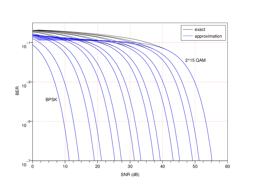
Figure 1: Exact BER curves and approximations (26).

III-B Dissimilar allocation measure

To measure the difference in the bit distribution between different allocation strategies, we need to evaluate the dissimilarity. This dissimilarity measure must verify the following properties: 1) if two allocations lead to the same bit distribution then the measure of dissimilarity must be null, whereas 2) if two allocations lead to two completely different bit distributions in loaded subchannels, then the measure of dissimilarity must be equal to one, and 3) the measure is symmetric, i.e. the dissimilarity between allocation $X$ and allocation $Y$ must be the same as the dissimilarity between allocation $Y$ and allocation $X$. We choose that the empty subchannels do not impact the measure.

Definition 1

The dissimilarity measure between allocation $X$ and allocation $Y$ is

$$\mu(X,Y)=\frac{\displaystyle\sum_{i=1}^{n}\delta\Big{(}r_{i}(X)-r_{i}(Y)\Big{)}}{\displaystyle\max_{j\in\{X,Y\}}\sum_{i=1}^{n}\delta\Big{(}r_{i}(j)\Big{)}}$$

where $\delta(x)=1$ if $x\neq 0$ else $\delta(x)=0$.

This dissimilarity has the following properties.

Property 1

$\mu(X,Y)=0$ iff $\forall i$, $r_{i}(X)=r_{i}(Y)$.

Property 2

$\mu(X,Y)=1$ iff $\forall i$ then $r_{i}(X)\neq r_{i}(Y)$ or $r_{i}(X)=r_{i}(Y)=0$.

Property 3

$\mu(X,Y)=\mu(Y,X)$.

Property 4

If $\mu(X,Y)=0$, then for all allocation $Z$, $\mu(X,Z)=\mu(Y,Z)$.

All these properties are direct consequences of Definition 1. For a null dissimilarity, $\mu(X,Y)=0$, all the subchannels transmit the same number of bits, i.e. $\forall i$ $r_{i}(X)=r_{i}(Y)$. For a full dissimilarity, $\mu(X,Y)=1$, all the non empty subchannels of both allocations $X$ and $Y$ transmit a different number of bits, i.e. $\forall i$ such as $r_{i}(X)\neq 0$ and $r_{i}(Y)\neq 0$ then $r_{i}(X)\neq r_{i}(Y)$. It is obvious that the measure is symmetric $\mu(X,Y)=\mu(Y,X)$. If two allocations have a null dissimilarity $\mu(X,Y)=0$, then they are identical and for any allocation $Z$ $\mu(X,Z)=\mu(Y,Z)$. The converse of this last property is not true. Note that the dissimilarity is not defined for two empty allocations.

For example, let $n=4$ and $[r_{1}(X),\cdots,r_{4}(X)]=[4\;3\;3\;0]$. If $[r_{1}(Y),\cdots,r_{4}(Y)]=[3\;2\;2\;2]$ or $[r_{1}(Y),\cdots,r_{4}(Y)]=[5\;5\;0\;0]$ then $\mu(X,Y)=1$. If $[r_{1}(Y),\cdots,r_{4}(Y)]=[4\;3\;2\;1]$ then $\mu(X,Y)=\frac{1}{2}$. The measure $\mu(X,Y)$ is null if and only if $[r_{1}(Y),\cdots,r_{4}(Y)]=[4\;3\;3\;0]$.

III-C Generalized secant method

There are many numerical methods for finding roots of function. We propose a new method, called generalized secant method that is based on secant method. This new method better fits the function-depending weight than secant method to speed the convergence. Before explaining this new method, a brief overview of secant method is given.

In our case, the objective function $f(x)$ is monotonous, non differentiable and computable over $x\in[x_{1},x_{2}]$ with $\frac{f(x_{1})}{|f(x_{1})|}=-\frac{f(x_{2})}{|f(x_{2})|}$. The secant method is as follows for an increasing function $f(x)$.

1. $i=0$, $y_{0}=f(x_{1})$;

2. $x_{0}=\frac{x_{2}f(x_{1})-x_{1}f(x_{2})}{f(x_{1})-f(x_{2})}$, $y_{i+1}=f(x_{0})$;

3. If $|y_{i+1}-y_{i}|\leq\epsilon$ then $x_{0}$ is the root of $f(x)$, else $\left\{\begin{array}[]{l}y_{i+1}<0\text{ then }x_{1}=x_{0}\\ y_{i+1}>0\text{ then }x_{2}=x_{0}\end{array}\right\}$, $i\to i+1$ and go to step 2.

The objective of the secant method is to approximate $f(x)$ by a linear function $g_{i}(x)=a_{i}x+b_{i}$ at each iteration $i$, with $g_{i}(x_{1})=f(x_{1})$ and $g_{i}(x_{2})=f(x_{2})$, and to set $x_{0}$ as the root of $g_{i}(x)$. The search for the root of $f(x)$ is completed when the desired precision $\epsilon$ is reached. The precision is given for $y_{i}$ but it can also be given for $x_{i}$.

As the function $f(x)$ is computable, it can be plotted and an a posteriori simple algebraic or elementary transcendental invertible function over $[x_{1},x_{2}]$ can be used to better fit the function $f(x)$. An a posteriori information is then used to improve the search for the root. The function $f(x)$ is iteratively approximated by $a_{i}h(x)+b_{i}$ instead of $a_{i}x+b_{i}$, where $h(x)$ is the invertible function. This method is then given as follows for an increasing function $f(x)$.

1. $i=0$, $y_{0}=f(x_{1})$;

2. $x_{0}=h^{-1}\Big{(}\frac{x_{2}f(x_{1})-x_{1}f(x_{2})}{f(x_{1})-f(x_{2})}\Big{)}$, $y_{i+1}=f(x_{0})$;

3. If $|y_{i+1}-y_{i}|\leq\epsilon$ then $x_{0}$ is the root of $f(x)$, else $\left\{\begin{array}[]{l}y_{i+1}<0\text{ then }x_{1}=x_{0}\\ y_{i+1}>0\text{ then }x_{2}=x_{0}\end{array}\right\}$, $i\to i+1$ and go to step 2.

Compared to secant method, only step 2) differs from generalized secant method where the computation of $x_{0}$ is performed taking into account the approximated shape $h(x)$ of the function $f(x)$.

This generalized secant method is used in Section V to find the root of the Lagrangian and is compared to the conventional secant method. In our case, $f(x)$ is the sum of logarithmic functions and the function $h(x)$ is then the logarithmic one.

IV Optimal greedy-type allocations

The general problem is to find the optimal allocation $[r_{1}^{*},\cdots,r_{n}^{*}]$ that minimizes $\phi(\cdot)$, the inverse robustness measure, or frailness. This is a combinatorial optimization problem or integer programming problem. The core idea in this iterative allocation is that a sequential approach can lead to a globally optimum discrete loading. Greedy-type methods then converge to optimal solution under conditions. Convexity is not required for the convergence of the algorithm and monotonicity is sufficient [31]. This monotonicity ensures that the removal or addition of $\beta$ bits at each iteration converges to the optimal solution. In this paper the used functions $\phi(\cdot)$ are monotonic increasing functions.

In its general form and when the objective function $\phi(\cdot)$ is not only a weighted sum function, the iterative algorithm is

1. Start with allocation $[r_{1}^{(0)},\cdots,r_{n}^{(0)}]=0$,

2. $k=0$,

3. Allocate one more bit to the subchannel $j$ for which

   $$\phi\Big{(}\{r_{i}^{(k+1)}\}_{i=1}^{n}\Big{)}$$ (28)

   is minimal, with $r_{j}^{(k+1)}=r_{j}^{(k)}+\beta$ and $\forall i\neq j$ $r_{i}^{(k+1)}=r_{i}^{(k)}$,

4. If $\sum_{i}r_{i}^{(k+1)}=R$, terminate; otherwise $k\to k+1$ and go to step 3.

The obtained allocation is then optimal [31] and solves (14). This algorithm needs $R/\beta$ iterations and its complexity is $\mathcal{O}(nR)$. The target bit-rate $R$ is supposed to be feasible, i.e. $R$ is a multiple of $\beta$. Note that an equivalent formulation can be given starting with $r_{i}^{(0)}=r_{\text{max}}$ for all $i$ and using bit-removal instead of bit-addition with maximization instead of minimization. For very high bit-rate, higher than $\frac{n}{2}r_{\text{max}}$, the number of iterations with bit-removal is lower than those obtained with bit-addition. This is the opposite with bit-rate lower than $\frac{n}{2}r_{\text{max}}$.

Iterative allocations have been firstly applied to bit-rate maximization under power constraint [13]. Many works have been devoted to complexity reduction of greedy-type algorithms, see for example [32, 33, 14, 8] and references therein. In this section, only greedy-type algorithms are presented in order to compare the analytical allocation to the optimal iterative one. Note that analytical solution can also be used as an input of greedy-type algorithm to initialize it and reduce its complexity.

IV-A System margin maximization

The system margin, or system SNR-gap, maximization under bit-rate and peak-power constraints is the converse problem of the bit-rate maximization under SNR-gap and peak-power constraints. This converse problem has been solved, e.g., in [20]. To comply with the general problem formulation, the inverse system margin minimization is presented instead of the system margin maximization.

Lemma 2

Under bit-rate and peak-power constraints, the greedy-type allocation that minimizes the inverse system margin $\gamma^{-1}$ (16) allocates sequentially $\beta$ bits to the subchannel $i$ bearing $r_{i}$ bits and for which

$$\frac{2^{r_{i}+\beta}-1}{\mathsf{snr}_{i}}$$

is minimum.

Proof:

It is straightforward using (17) and (28). See Appendix A for an original proof. ∎

The main advantage of system margin maximization is that the optimal allocation can be reached independently of the SNR regime. Allocation is always possible even for very low SNR but it can lead to unreliable communication with SNR-gap lower than 1. Lemma 2 is given with unbounded modulation orders, i.e. $r_{\text{max}}=\infty$ and $\forall i$ $r_{i}\in\beta\mathbb{N}$. With full constraints (13), the subchannels that reach $r_{\text{max}}$ are simply removed from the iterative process.

IV-B BER minimization

The system BER minimization under bit-rate and peak-power constraints is the converse problem of bit-rate maximization under peak-power and BER constraints. This converse problem has been solved, e.g., in [25]. Using (28) and (24), the solution of BER minimization is straightforward and the corresponding greedy-type algorithm is also known as Levin-Campello algorithm [7, 34, 35]. The main drawback of this solution is that it requires good approximated BER expressions even in low SNR regime. This constraint can be relaxed and the following lemma gives the optimal greedy-type allocation for the BER minimization.

Lemma 3

In high SNR regime and under bit-rate and peak-power constraints, the greedy-type allocation that minimizes the BER minimizes $(r_{i}+\beta)\mathsf{ber}_{i}(r_{i}+\beta)$ at each step.

Proof:

See Appendix B. ∎

Lemma 3 states how to allocate bits without mean BER computation at each step. It is given without modulation order limitation. Like system margin maximization solution, the bounded modulation order is simply taken into account using $r_{\text{max}}$ and subchannel removal.

IV-C Comparison of allocations

To compare the two optimization policies, we call $\mathcal{B}$ the allocation that maximizes the system margin and $\mathcal{C}$ the allocation that minimizes the BER. Table I gives an example of bit-rate allocation over 20 subchannels where the SNR follows a Rayleigh distribution and with $\beta=1$. In this example the PSDNR is equal to 25 dB and the maximum allowed bit-rate per subchannel is never reached. As expected, the system margin minimization leads to a minimal SNR-gap, $\min_{i}\gamma_{i}$, higher than that provided by the BER minimization policy with a gain of 0.3 dB. On the other hand, the BER minimization policy leads to BER lower than that provided by system margin minimization ($2.6\cdot 10^{-5}$ versus $3.1\cdot 10^{-5}$). In this example, the dissimilarity is $\mu(\mathcal{B,C})=0.1$ and two subchannels convey different bit-rates. All these results are obtained with $r_{\text{max}}=10$.

TABLE I: Example of system margin and BER with $n=20$, $R=100$, $\mathsf{psdnr}=25~{}\mathrm{dB}$ and $\beta=1$.

	system margin	BER
	maximization	minimization
	($\mathcal{B}$)	($\mathcal{C}$)
$\min\limits_{i}\gamma_{i}$	6.9 dB	6.6 dB
$\mathsf{ber}$	$3.1\cdot 10^{-5}$	$2.6\cdot 10^{-5}$

This example shows that the difference between the two allocation policies is not so important. The question is whether both allocations converge and if they converge then in what case. The following theorem answers the question.

Theorem 1

In high SNR regime with square QAM and under bit-rate and peak-power constraints, the greedy-type allocation that maximizes the system margin converges to the greedy-type allocation that minimizes the BER.

Proof:

See Appendix D. ∎

The consequence of Theorem 1 is that the dissimilarity between allocation that maximizes the system margin and allocation that minimizes the BER is null in high SNR regime and with square QAM. With square QAM, $\beta$ should be a multiple of 2. Note that with square modulations, $\beta$ can also be equal to 1 if the modulations are, for example, those defined in ADSL [36]. Fig. 5 exemplifies the convergence with $\beta=2$ as we will see later in Section VI.

V Optimal analytical allocations

The analytical method is based on convex optimization theory [37]. Unconstrained modulations lead to bit-rates $r_{i}$ defined in $\mathbb{R}$. With $r_{i}\in\mathbb{R}_{+}$ the solution is the waterfilling one. With bounded modulation order, i.e. $0\leq r_{i}\leq r_{\text{max}}$, the solution is quite different from the waterfilling one. The solution is obtained in the framework of generalized Lagrangian relaxation using Karush-Kuhn-Tucker (KKT) conditions [38].

As the bit-rates are continuous and not only integers, the constraints (13) do not hold anymore and become

$$\sum_{i=1}^{n}r_{i}=R\quad\forall i\ 0\leq r_{i}\leq r_{\text{max}}\ .$$ (29)

The KKT conditions associated to the general problem (14) with (29) instead of (13) write [38]

$$-r_{i} \leq 0\,,\ \forall i\in[1,n]$$ (30)

$$r_{i}-r_{\text{max}} \leq 0\,,\ \forall i\in[1,n]$$ (31)

$$R-\sum\limits_{i=1}^{n}r_{i} =0$$ (32)

$$\mu_{i} \geq 0\,,\ \forall i\in[1,n]$$ (33)

$$\nu_{i} \geq 0\,,\ \forall i\in[1,n]$$ (34)

$$\mu_{i}r_{i} =0\,,\ \forall i\in[1,n]$$ (35)

$$\nu_{i}(r_{i}-r_{\text{max}}) =0\,,\ \forall i\in[1,n]$$ (36)

$$\frac{\partial}{\partial r_{i}}\phi\Big{(}\{r_{j}\}_{j=1}^{n}\Big{)}-\lambda-\mu_{i}+\nu_{i} =0\,,\ \forall i\in[1,n]$$ (37)

The first three conditions (30)–(32) represent the primal constraints, conditions (33) and (34) represent the dual constraints, conditions (35) and (36) represent the complementary slackness and condition (37) is the cancellation of the gradian of Lagrangian with respect to $r_{i}$. When the primal problem is convex, i.e. $\phi\big{(}\{r_{i}\}_{i=1}^{n}\big{)}$ is convex and the constraints are linear, the KKT conditions are sufficient for the solution to be primal and dual optimal. For the system margin maximization problem, the function $\phi(\cdot)$ is convex over all input bit-rates and SNR whereas this function is no more convex for the BER minimization problem. Appendix C gives the convex domain of the function $\phi(\cdot)$ in the case of BER minimization problem.

The properties of the studied function $\phi(\cdot)$ are such that

$$\frac{\partial}{\partial r_{i}}\phi\Big{(}\{r_{j}\}_{j=1}^{n}\Big{)}=\psi_{i}(r_{i})\ .$$ (38)

The optimal solution that solve (30)–(37) is then [38]

$$r_{i}^{*}(\lambda)=\left\{\begin{array}[]{l@{\quad\text{if}\quad}l}0&\lambda\leq\psi_{i}(0)\\ \psi_{i}^{-1}(\lambda)&\psi_{i}(0)<\lambda<\psi_{i}(r_{\text{max}})\\ r_{\text{max}}&\lambda\geq\psi_{i}(r_{\text{max}})\end{array}\right.$$ (42)

for all $i\in[1,n]$ and with $\lambda$ verifying the constraint

$$\sum_{i=1}^{n}r_{i}^{*}(\lambda)=R\ .$$ (43)

It is worthwhile noting that the above general solution is the waterfilling one if $r_{\text{max}}\geq R$. The waterfilling is also the solution in the following case. Let $\mathcal{I}^{\prime}$ the subset such that $\forall i\in\mathcal{I}^{\prime}$, $r_{i}^{*}\notin\{0,r_{\text{max}}\}$ and let $R^{\prime}$ the target bit-rate over $\mathcal{I}^{\prime}$. In this subset, $\{r_{i}^{*}\}_{i\in\mathcal{I}^{\prime}}$ are solutions of

$$\left\{\begin{array}[]{r@{\ =\ }l}\frac{\partial}{\partial r_{i}}\phi\Big{(}\{r_{j}\}_{j=1}^{n}\Big{)}-\lambda&0\,,\ \forall i\in\mathcal{I}^{\prime}\\ R^{\prime}-\sum\limits_{i\in\mathcal{I}^{\prime}}r_{i}(\lambda)&0\end{array}\right.$$ (46)

This is the solution of (14) with unbounded modulations over the subchannel index subset $\mathcal{I}^{\prime}$. If $\mathcal{I}^{\prime}=\{1,\cdots,n\}$ and $R^{\prime}=R$, (46) is also the solution of (14) with unconstrained modulations.

V-A System margin maximization

Theorem 2

Under bit-rate and peak-power constraints, the asymptotic bit allocation with unconstrained modulations which minimizes the inverse system margin is given by

$$\forall i\in[1,n],\quad r_{i}^{*}=\frac{R}{n}+\frac{1}{n}\sum_{j=1}^{n}\log_{2}\frac{\mathsf{snr}_{i}}{\mathsf{snr}_{j}}$$

Proof:

See Appendix E. ∎

The solution given by Theorem 2 holds for high modulation orders which defines the asymptotic regime, cf. Appendix E. As the modulations are unconstrained, the bit-rates $\{r_{i}^{*}\}_{i=1}^{n}$ are real numbers defined in $\mathbb{R}$. With bounded modulation orders, Theorem 2 is used into (42) to solve (14) with constraints (29). If the set $\mathcal{I}^{\prime}$ is known, then Theorem 2 can be used directly to allocate the subchannel bit-rates. Otherwise $\mathcal{I}^{\prime}$ should be found first.

The expression of $r_{i}^{*}$ in Theorem 2 is a function of the target bit-rate $R$, the number $n$ of subchannels and the ratios of SNR. This expression is independent of mean received SNR or PSDNR. It does not depend on link budget but only on relative distribution of subchannel coefficients $\{|h_{i}|^{2}\}_{i=1}^{n}$.

V-B BER minimization

The arithmetic mean BER minimization has been analytically solved for example in [24, 39]. This arithmetic mean measure needs to employ the same number of bits per constellation which limits the system efficiency. The following theorem gives the solution of the weighted mean BER minimization that allows variable constellation sizes in the multichannel system.

Theorem 3

Under bit-rate and peak-power constraints, the asymptotic bit allocation with unconstrained QAM which minimizes the BER is given by

$$\forall i\in[1,n],\quad r_{i}^{*}=\frac{R}{n}+\frac{1}{n}\sum_{j=1}^{n}\log_{2}\frac{\mathsf{snr}_{i}}{\mathsf{snr}_{j}}$$

with equal in-phase and quadrature bit-rates.

Proof:

See Appendix F. ∎

The solution given by Theorem 3 holds for high modulation orders and for subchannel BER lower than 0.1, and these parameters define the asymptotic regime in this case, cf. Appendix F. The optimal asymptotic allocation leads to square QAM with $\sqrt{r_{i}^{*}}$ conveyed bit-rate in each in-phase and quadrature components of the signal of subchannel $i$. With bounded modulation orders, Theorem 3 is used in (42) to solve (14) with constraints (29). It is important to note that in asymptotic regime, BER minimization and system margin maximization lead to the same subchannel bit-rate allocation. In that case, the asymptotic regime is defined by the more stringent context which is the BER minimization. As we will see in Section VI, this asymptotic behavior can be observed when $\beta=2$.

The main drawback of the formulas in Theorem 3 and Theorem 2 is that the bit-rates $\{r_{i}^{*}\}_{i=1}^{n}$ are expressed in $\mathbb{R}$ and not in $\mathbb{R}_{+}$. To find the set $\mathcal{I}^{\prime}$, the negative subchannel bit-rates and those higher than $r_{\text{max}}$ should be clipped and $\mathcal{I}^{\prime}$ can be found iteratively [20]. But clipping negative bit-rates first can decrease those higher than $r_{\text{max}}$ and clipping bit-rates higher than $r_{\text{max}}$ first can increase the negative ones. It is then not possible to apply first the waterfilling solution and after that to clip the bit-rates $r_{i}$ greater than $r_{\text{max}}$ to converge to the optimal solution. Finding the set $\mathcal{I}^{\prime}$ requires many comparisons and we propose a fast iterative solution based on generalized secant method.

V-C Lagrangian resolution

To solve (42), numerical iterative methods are required. It is important to observe that the function defined in (42) is not differentiable and thus, methods like Newton’s cannot be used [20]. We use the proposed generalized secant method to better fit the function-depending weight and increase the speed of the convergence. An important point for the iterative method is that the initialization must embrace all possible scenarios and should be as close as possible to the final solution.

The root of the function defined by (43) is now calculated. Let

$$f(\lambda)=\sum_{i=1}^{n}r_{i}(\lambda)-R\,.$$ (47)

Theorems 2 and 3 show that $r(\lambda)$ is the sum of $\log_{2}(\cdot)$ functions. This is the reason why the function $\log_{2}(\cdot)$ is used in generalized secant method. Fig. 2 shows three functions versus the parameter $\lambda$. The first function is the input function $f(\lambda)$, the second one is the function used by the generalized secant method, and the last one if the linear function used by the secant method. In this example, the common points are $\lambda=0$ and $\lambda=2.3$. As it is shown, the generalized secant method better fit the input function than the secant method and therefore can improve the speed of the convergence to find the root which is around $\lambda=1/80$ in this example.

To ensure the non empty root of the input function $f(\lambda)$, the secant methods should be initialized with $\lambda_{1}$ and $\lambda_{2}$ such as $f(\lambda_{1})<0$ and $f(\lambda_{2})>0$. For both optimization problems, system margin maximization and BER minimization, the parameter $\lambda$ is given by the function $\psi_{i}(r_{i})$ and it can be reduced to $\lambda=\frac{2^{r_{i}}}{\mathsf{snr}_{i}}$, as shown in appendices E and F. Parameters $\{\lambda_{1},\lambda_{2}\}$ are then chosen as

$$\lambda_{1}=\frac{1}{\max\limits_{i}\mathsf{snr_{i}}}\quad\text{and}\quad\lambda_{2}=\frac{2^{r_{\text{max}}}}{\min\limits_{i}\mathsf{snr_{i}}}\,.$$ (48)

Using (42), $\lambda\leq\lambda_{1}$ leads to $r_{i}(\lambda)=0$ for all $i$, and $\lambda\geq\lambda_{2}$ leads to $r_{i}(\lambda)=r_{\text{max}}$ for all $i$. Then, it follows that $f(\lambda_{1})<0$ and $f(\lambda_{2})>0$ if $R\in(0,nr_{\text{max}})$.

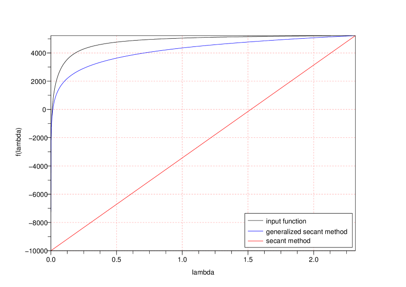
Figure 2: Approximation of input function $f(\lambda)$ with generalized secant method and secant method, $n=1024$ and $r_{\text{max}}=15$.

Fig. 3 shows the needed number of iterations for the convergence of the generalized and conventional secant methods versus the target bit-rate $R$. Results are given over a Rayleigh distribution of the subchannel SNR with 1024 subchannels. The possible bit-rates are then $R\in[0,n\times r_{\text{max}}]$ and $\beta=2$. Here, $r_{\text{max}}=15$ and then $R\leq 15360$ bits per multidimensional symbol. For comparison, the number of iterations needed by the greedy-type algorithm is also plotted. Note that the greedy-type algorithm can start by empty bit-rate or by full bit-rate limited by $r_{\text{max}}$ for each subchannel. The number of iterations is then given by $\min\{R,nr_{\text{max}}-R\}$. The iterative secant and generalized secant methods are stopped when the bit-rate error is lower than 1. A better precision is not necessary since exact bit-rates $\{r_{i}\}_{i\in\mathcal{I}^{\prime}}$ can be computed using Theorems 2 and 3 when $\mathcal{I}^{\prime}$ is known. As it is shown in Fig. 3, the generalized secant method converges faster than the secant method, except for the very low target bit-rates $R$. For very high target bit-rates, near from $n\times r_{\text{max}}$, generalized secant method can lead to a number of iterations higher than those of greedy-type algorithm. Except for these particular cases, the generalized secant method needs no more than 4–5 iterations to converge. In conclusion, we can say that with Rayleigh distribution of $\{\mathsf{snr}_{i}\}_{i=1}^{n}$, the generalized secant method converges faster than secant method or greedy-type algorithm for target bit-rate $R$ such that $3\%\leq\frac{R}{nr_{\text{max}}}\leq 97\%$.

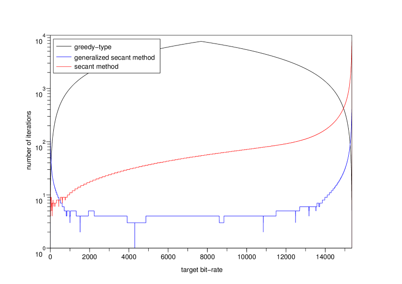
Figure 3: Number of iterations of secant and generalized secant methods, and greedy-type algorithm versus the target bit-rate, $n=1024$, $r_{\text{max}}=15$.

Using generalized secant method the bit-rates are not integer and for all $i$, $r^{*}_{i}\in[0,r_{\text{max}}]$. These solutions have to be completed to obtain integer bit-rates.

V-D Integer-bit solution

Starting from continuous bit-rates allocation previously presented, a loading procedure is developed taking into account the integer nature of the bit-rates to be allotted. A simple solution is to consider the integer part of $\{r_{i}^{*}\}_{i\in\mathcal{I}^{\prime}}$ and to complete by a greedy-type algorithm to achieve the target bit-rate $R$. The integer part of $\{r_{i}^{*}\}_{i\in\mathcal{I}^{\prime}}$ is then used as a starting point for the greedy algorithm. This procedure can lead to a high number of iterations, therefore the secant or bisection methods are suitable to reduce the complexity. The problem to solve is then to find the root of the following function [20]

$$g(\alpha)=\sum_{i\in\mathcal{I}^{\prime}}\lfloor r_{i}^{*}+\beta\alpha\rfloor-R^{\prime}\,,$$ (49)

where $r_{i}^{*}$, $\mathcal{I}^{\prime}$ and $R^{\prime}$ are given by the continuous Lagrangian solution. This is a suboptimal integer bit-rate problem and the optimal one needs to find $\{\alpha_{i}\}_{i=1}^{n}$ instead of a unique $\alpha$. As the optimal solution leads to a huge complexity, it is not considered. The function (49) is a non decreasing and non differentiable staircase function such that $g(0)<0$, $g(1)>0$ because $\sum_{i\in\mathcal{I}^{\prime}}r_{i}^{*}=R^{\prime}$. The iterative methods can then be initialized with $\alpha_{1}=0$ and $\alpha_{2}=1$.

Two iterative methods are compared, the bisection one and the secant one. Both methods are also compared to the greedy-type algorithm. Fig. 4 presents the number of iterations of the three methods to solve the integer-bit problem of the Lagrangian solution with $\beta=1$. Results are given over a Rayleigh distribution of the subchannel SNR, with 1024 subchannels and the target bit-rates are between 0 and $n\times r_{\text{max}}=15360$. As it is shown, the convergence is faster with bisection method than with greedy-type algorithm. For target bit-rates between 10% and 90% of the maximal loadable bit-rate, the secant method outperforms the bisection one with a mean number of iterations around 4 whereas the number of iterations for bisection method is higher than 8. Fig. 4 also shows that $|g(0)|$ is all the time lower than the half of number of subchannels and around this value for target bit-rate between 10% and 90% of the maximal loadable bit-rate. Then, if the complexity induces by the greedy-type algorithm to solve the integer-bit problem of the Lagrangian solution is acceptable in a practical communication system, this greedy-type completion can be used and leads to the optimal allocation. This result obtained without proof means that the greedy-type procedure has enough bits to converge to the optimal solution. If the number of iterations induced by the greedy-type algorithm is too high (this number is around $n/2$), the secant method can be used.

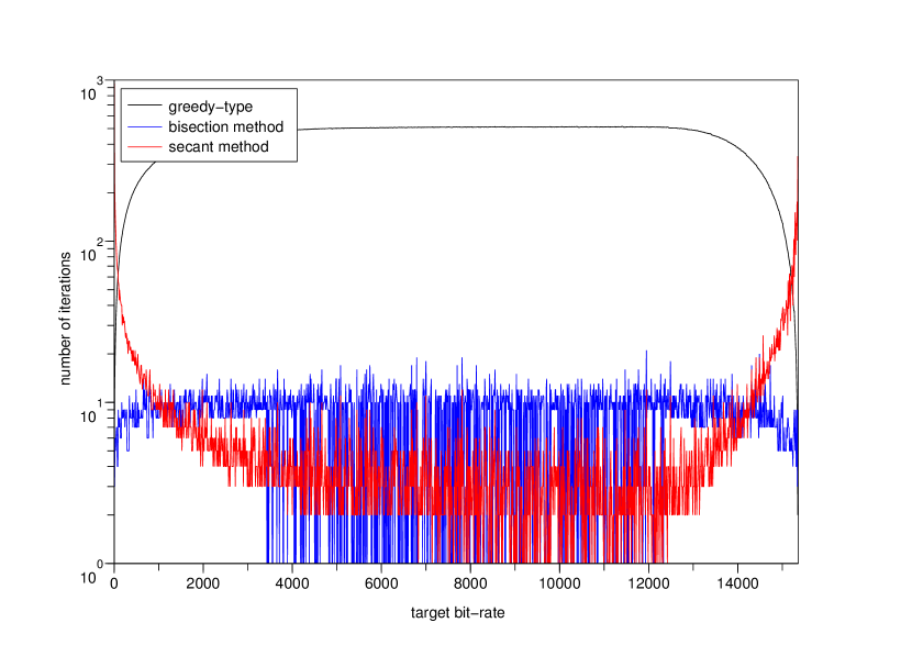
Figure 4: Number of iterations of bisection and secant methods, and greedy-type algorithm for integer-bit solution versus target bit-rate, $n=1024$, $r_{\text{max}}=15$.

The overall analytical resolution of (14) needs few iterations and its complexity is $\mathcal{O}(n)$ instead of $\mathcal{O}(Rn)$ for the optimal greedy-type algorithm. Whereas the continuous solution of (14) is optimal, the analytical integer bit-rate solution is suboptimal.

VI Greedy-type versus analytical allocations

In the previous section, algorithm complexities have been compared. In this section, robustness comparison is presented and the analytical solutions obtained in asymptotic regime are also applied in non asymptotic regime which means that $\beta=1$ and modulation orders can be low.

Figure 5: BER, system margin and dissimilarity versus target bit-rate for Lagrangian ($\mathcal{A}$), greedy-type system margin maximization ($\mathcal{B}$) and greedy-type BER minimization ($\mathcal{C}$) algorithms, $n=1024$, $r_{\text{max}}=14$, $\beta\in\{1,2\}$.

Fig. 5 presents the output BER and the system margin of three allocation policies versus the target bit-rate $R$. The first one, $\mathcal{A}$, is obtained using analytical optimization, the second, $\mathcal{B}$, is the solution of the greedy-type algorithm which maximizes the system margin and the third, $\mathcal{C}$, is the solution of the greedy-type algorithm which minimizes the BER. Two cases are presented, one with $\beta=1$ and the other with $\beta=2$. All subchannel BER are lower than $2\cdot 10^{-2}$ to use valid BER approximations. To compare the case $\beta=1$ with the case $\beta=2$, $r_{\text{max}}$ is equal to 14. Results are given over a Rayleigh distribution of the subchannel SNR, with 1024 subchannels. Note that with $\beta=1$, the system margin of allocation $\mathcal{B}$ is almost equal to 8.9 dB for all target-bit rates. This constant system margin $\gamma$ is not a feature of the algorithm but is only a consequence of the relation between the target bit-rate and the PSDNR.

To enhance the equivalences and the differences between the allocation policies, the dissimilarity is also given in Fig. 5 with $\beta=1$ and $\beta=2$. As expected and in both cases $\beta=1$ and $\beta=2$, the minimal BER are obtained with allocation $\mathcal{C}$, and the maximal system margins with allocation $\mathcal{B}$. With $\beta=1$ and when the target bit-rate increases, the Lagrangian solution converges faster to the optimal system margin maximization solution $\mathcal{B}$ than to the optimal BER minimization solution $\mathcal{C}$. Note that Theorem 3 is an asymptotic result valid for square QAM. With $\beta=1$, the QAM can be rectangular and the asymptotic result of Theorem 3 is not applicable, contrary to the result of Theorem 2 where there is not any condition on the modulation order. With $\beta=2$, the modulation granularity is lower and then the output BER are higher than those obtained with $\beta=1$, as the output system margins are lower than those obtained with $\beta=1$. This case $\beta=2$ shows the equivalence between the optimal system margin maximization allocation and the optimal BER minimization allocation. In this case, the asymptotic result given by Theorem 1 and 3 can be applied because the modulations are square QAM, and the convergence is ensured with high modulation orders, i.e. high target bit-rates. Beyond a mean bit-rate per subchannel around 10, that corresponds to a target bit-rate around $10^{4}$, all the allocations $\mathcal{A}$, $\mathcal{B}$ and $\mathcal{C}$ are equivalent and the dissimilarity is almost equal to zero. In non asymptotic regime, the differences in BER and system margin are low. The system margin differences are lower than 1 dB, and the ratios between two BER are around 3. In practical integrated systems these low differences will not be significant and will lead to similar solutions for both optimization policies. Therefore, these allocation can be interchanged.

VII Application: DMT for power line channel

All previous results are presented over Rayleigh distribution of subchannel SNR. This distribution can occur in PLC channel [40] but distribution with higher SNR range is also possible [41]. The robustness is evaluated in harsh condition and the model proposed in [41] is then chosen. Fig. 6 shows the frequency response of 15 paths PLC model in $[0.5;20]$ MHz bandwidth where the subchannels undergo more than 60 dB SNR range. In PLC systems, the subchannels are the subcarriers of the multicarrier system and the PLC communication system uses 1024 subcarriers, $r_{\text{max}}=15$ as in xDSL communication systems and $\beta=1$. All QAM constellations between 4-QAM to 32768-QAM plus BPSK are used. Note that with 60 dB of SNR range, there are possible $r_{i}=0$ and $r_{j}=15$ in the same multicarrier symbol since around 45 dB of SNR range is sufficient to have both $r_{i}=0$ and $r_{j}=15$ in the same multicarrier symbol. The robustness measures are evaluated for different target bit-rates which are given with the following arbitrary equation

$$R=\left\lfloor\sum_{i=1}^{n}\min\Big{(}\log_{2}\big{(}1+\frac{\mathsf{snr}_{i}}{2}\big{)},r_{\text{max}}\Big{)}\right\rfloor\,.$$ (50)

This equation ensures reliable communications for all the input target bit-rates or PSDNR. The empirical relationship between PSDNR and target bit-rate is also given in Fig. 6.

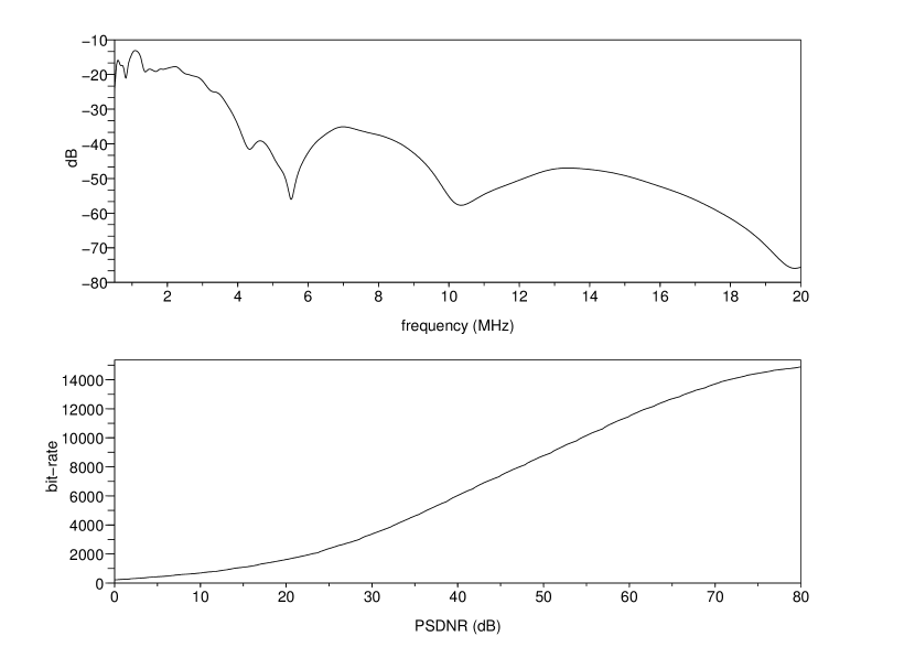
Figure 6: Frequency response of 15 paths PLC model [41] versus frequency and target bit-rate versus input PSDNR.

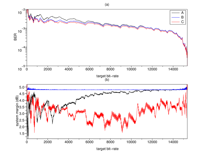
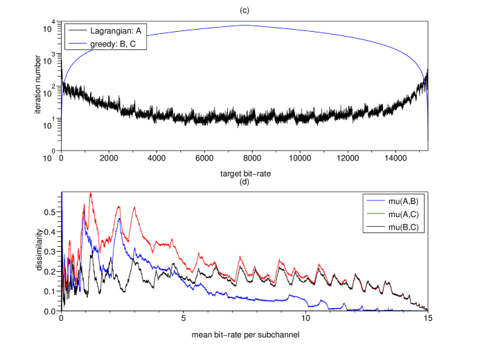
Figure 7: (a) BER, (b) system margin versus target bit-rate for Lagrangian ($\mathcal{A}$), greedy-type system margin maximization ($\mathcal{B}$) and greedy-type BER minimization ($\mathcal{C}$) algorithms, (c) iteration number of Lagrangian solution and greedy-type algorithms versus target bit-rate, and (d) dissimilarities $\mu(\mathcal{A,B})$, $\mu(\mathcal{A,C})$ and $\mu(\mathcal{B,C})$ versus mean bit-rate per subchannel, $n=1024$, $r_{\text{max}}=15$.

Fig. 7 sums up the characteristics and the results of three allocation policies in PLC context. The first allocation, $\mathcal{A}$, is obtained using analytical optimization developed in Section V, the second, $\mathcal{B}$, is the solution of the greedy-type algorithm given by Lemma 2 which maximizes the system margin and the third, $\mathcal{C}$, is the solution of the greedy-type algorithm given by Lemma 3 which minimizes the BER. In this figure, the BER, the system margin in decibel and the needed number of iterations are plotted versus the input target bit-rates, subfigure (a), (b) and (c) respectively. The subfigure (d) gives the dissimilarity measure versus the mean bit-rate per subchannel which is equal to $R/n$. In subfigure (a) the minimal BER is obtained with allocation $\mathcal{C}$, as expected. The allocation $\mathcal{A}$ offers the worse BER with a maximal ratio of 2 compared to the best result. For high bit-rates this ratio converges to 1. In subfigure (b) the maximal system margin is given by allocation $\mathcal{B}$, as expected,. The maximal difference between allocations $\mathcal{B}$ and $\mathcal{C}$ is around 3 dB. The number of iterations needed with Lagrangian method, allocation $\mathcal{A}$, is very low compared with optimal greedy-type ones, allocations $\mathcal{B}$ and $\mathcal{C}$. Subfigure (c) shows that only 20 iterations are sufficient for most cases to perform allocation with method $\mathcal{A}$, when up to 7680 iterations are needed with greedy-type algorithms. This maximal number of iterations is given by $\frac{n}{2}r_{\text{max}}$. The dissimilarity, subfigure (d), is very high for low mean bit-rate per subchannel. When the mean number of bits per constellation is low, the asymptotic results do not hold. This dissimilarity decreases with the increase of the mean bit-rate per subchannel where the asymptotic results become valid. Note that as the PSDNR varies with the target bit-rate, the BER curves are not simply decreasing and the system margin curves are not simply increasing with the increase of the target bit-rate.

All these results show that the allocation $\mathcal{A}$ based on Lagrangian method converges faster to allocation $\mathcal{B}$ (than to allocation $\mathcal{C}$) when the bit-rate increases. In communication systems with $\beta=1$, the asymptotic conditions of analytical solution of minimal BER problem do not hold. Nevertheless, the difference between allocations $\mathcal{A}$ and $\mathcal{C}$ remains low. The system margin differences are up to 3.5 dB, and the BER ratios are up to 2.2. The allocation policy should then be selected depending on the considered robustness measure.

Fig. 5 and 7, and complementary simulations not presented here, show that the system margin difference between two allocation policies increases when the average value of the system margin decreases, whereas the BER difference, or ratio, between two allocation policies decreases when the average value of system BER increases. With optimized uncoded systems, the case presented in Fig. 7 is generally considered for operating points which correspond to higher BER. Both allocation policies then lead to similar BER performance but lead to significantly different system margin performance.

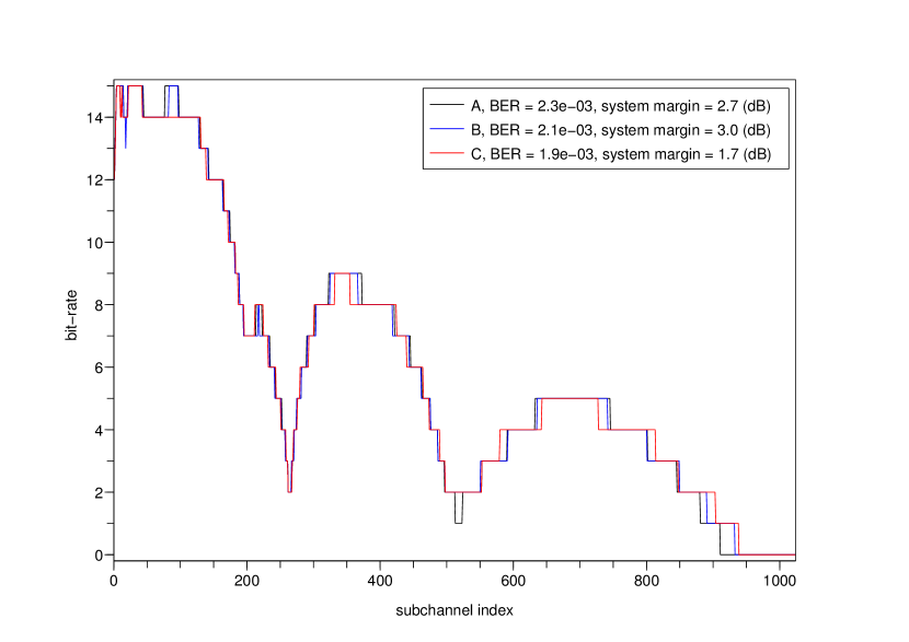
Figure 8: Example of bit-rate allocation versus subchannel index for Lagrangian ($\mathcal{A}$), greedy-type system margin maximization ($\mathcal{B}$) and greedy-type BER minimization ($\mathcal{C}$) algorithms, $n=1024$, $r_{\text{max}}=15$, $\mathsf{psdnr}=40$ dB, $R=6030$.

Fig. 8 gives an example of bit-rate distribution between subchannels with an input bit-rate of 6030 bits per multicarrier symbol which corresponds to a PSDNR of 40 dB. All the bit-rate distributions follow the shape of the PLC channel frequency response and exhibit some variations. In this example, the system margin of the allocation $\mathcal{A}$ is close to the optimal one, and is between the system margin of the two greedy-type solutions. Allocation $\mathcal{A}$ offers the highest BER but only 1.2 times higher than the optimal BER. The main difference between allocations $\mathcal{B}$ and $\mathcal{C}$ is the distribution of even and odd number of bits per constellation. With allocation $\mathcal{B}$ there are almost as many odd elements as there are even, whereas allocation $\mathcal{C}$ favors even elements. This behavior of allocation $\mathcal{C}$ is exemplified in Fig. 8 with $r_{i}=4$ and subchannel index $i$ around 600 and 800, or with $r_{i}=8$ and $i$ around 400. The explanation is given by the BER curves in Fig. 1 where the distance between two curves depends on the parity of the number of bits per constellation. The distance between the curves corresponding to $r_{i}=3$ and $r_{i}=4$ is lower than the distance for the case $r_{i}=4$ and $r_{i}=5$. Then, for the same slope of the input frequency response function, the staircase function of the allocation $\mathcal{C}$ in Fig. 8 has larger step size when the numbers of bits per constellation are even.

All these results in PLC context show that both allocation policies, system margin maximization and BER minimization, lead to different bit-rate allocations. These unique allocations have significant system margin difference whereas the BER difference between these allocations is very low. The suboptimal analytical solution based on Lagrangian offers a good trade-off between performance and complexity. With channel coding, not taken into account in this paper, the analysis remains valid: the ultimate output coded BER is strongly related to the uncoded BER, and the system margin optimization is independent of channel coding type.

VIII Conclusion

Two robustness optimization problems have been analyzed in this paper. Weighted mean BER minimization and minimal subchannel margin maximization have been solved under peak-power and bit-rate constraints. The asymptotic convergence of both robustness optimizations has been proved for analytical and algorithmic approaches. In non asymptotic regime the allocation policies can be interchanged depending on the robustness measure and the operating point of the communication system. We have also proved that the equivalence between SNR-gap maximization and power minimization in conventional MM problem does not hold with peak-power limitation without additional conditions. Integer bit solution of analytical continuous bit-rates has been obtained with a new generalized secant method, and bit-loading solutions have been compared with a new defined dissimilarity measure. The low computational effort of the suboptimal solution, based on the analytical approach, leads to a good trade-off between performance and complexity.

Appendix A Proof of Lemma 2

We prove that the optimal allocation is reached starting from empty loading with the same intermediate loading than starting from optimal loading to empty loading. To simplify the notation and without loss of generality, $\beta=1$.

Let $[r_{1}^{*},\cdots,r_{n}^{*}]$ be the optimal allocation that minimizes the inverse system margin $\gamma(R^{*})^{-1}$ for the target bit-rate $R^{*}$, then

$$\gamma(R^{*})^{-1}=\max_{i}\frac{2^{r_{i}}-1}{\mathsf{snr}_{i}}\ .$$ (51)

Let $[r_{1},\cdots,r_{n}]$ be the optimal allocation that minimizes the inverse system margin $\gamma(R+1)^{-1}$ for the target bit-rate $R+1\leq R^{*}$. The optimal allocation for target bit-rate $R$ is obtained iteratively by removing one bit at a time from the subchannel $k$ with the highest inverse system margin [42]

$$k=\arg\max_{i}\frac{2^{r_{i}}-1}{\mathsf{snr}_{i}}$$ (52)

or

$$\forall i\in[1,n]\quad\frac{2^{r_{k}}-1}{\mathsf{snr}_{k}}\geq\frac{2^{r_{i}}-1}{\mathsf{snr}_{i}}\ .$$ (53)

The last bit removed is from the subchannel with the lowest inverse-SNR, $\mathsf{snr}_{i}^{-1}$, because the bits over the highest inverse-SNR are first removed.

Now, let $[r_{1},\cdots,r_{n}]$ be the optimal allocation that minimizes the inverse system margin $\gamma(R)^{-1}$ for the target bit-rate $R<R^{*}$. Following the algorithm strategy, the optimal allocation for target bit-rate $R+1$ is obtained adding one bit on subchannel $j$ such that

$$j=\arg\min_{i}\frac{2^{r_{i}+1}-1}{\mathsf{snr}_{i}}\ .$$ (54)

We first prove that

$$\gamma(R+1)^{-1}=\frac{2^{r_{j}+1}-1}{\mathsf{snr}_{j}}\ .$$ (55)

Suppose there exists $j^{\prime}$ such that

$$\frac{2^{r_{j^{\prime}}}-1}{\mathsf{snr}_{j^{\prime}}}>\frac{2^{r_{j}+1}-1}{\mathsf{snr}_{j}}\ ,$$ (56)

then one bit must be added to subchannel $j$ to obtain $r_{j}+1$ bits before adding one bit to subchannel $j^{\prime}$ to obtain $r_{j^{\prime}}$ bits which means that $[r_{1},\cdots,r_{n}]$ is not optimal. As $[r_{1},\cdots,r_{n}]$ is optimal by definition, it yields

$$\forall i\in[1,n]\quad\frac{2^{r_{i}}-1}{\mathsf{snr}_{i}}\leq\frac{2^{r_{j}+1}-1}{\mathsf{snr}_{j}}$$ (57)

which proves (55). The first allocated bit is from the subchannel with the lowest inverse-SNR given by (54) with $r_{i}=0$ for all $i$.

Comparing (53) with (57) yields that $k=j$, and the index subchannel of the first added bit is the same as the last removed bit. All the intermediate allocations are then identical with bit-addition and bit-removal methods. There exists only one way to reach the optimal allocation $R^{*}$ starting from the empty loading.

Proof of Lemma 2 can also be provided in the framework of matroid algebraic theory [21, 43].

Appendix B Proof of Lemma 3

To simplify the notation and without loss of generality the proof is given with $\beta=1$. Let $[r_{1},\cdots,r_{n}]$ be the optimal allocation for the target bit-rate $R$ such that $\sum r_{i}=R$. Let $R+1$ the new target bit-rate. We first prove that $\Delta_{i}(r_{i})=(r_{i}+1)\mathsf{ber}_{i}(r_{i}+1)-r_{i}\mathsf{ber}_{i}(r_{i})$ is a good measure at each step of the greedy-type algorithm for the BER minimization, and finally that $(r_{i}+1)\mathsf{ber}_{i}(r_{i}+1)$ can be used instead of $\Delta_{i}(r_{i})$.

Starting from the optimal allocation of target bit-rate $R$, the new target bit-rate $R+1$ is obtained by increasing $r_{j}$ by one bit

$$\mathsf{ber}(R+1)=\frac{(r_{j}+1)\mathsf{ber}_{j}(r_{j}+1)+\sum\limits_{\begin{subarray}{c}i=1\\ i\neq j\end{subarray}}^{n}r_{i}\mathsf{ber}_{i}(r_{i})}{1+\sum\limits_{i=1}^{n}r_{i}}$$ (58)

and, using $\Delta_{j}$,

$$\mathsf{ber}(R+1)=\frac{\Delta_{j}(r_{j})}{R+1}+\frac{R}{R+1}\mathsf{ber}(R)\,.$$ (59)

The $\mathsf{ber}(R+1)$ which is equal to $\phi(\{r_{i}^{(k+1)}\}_{i=1}^{n})$ in (28) is minimized only if $\Delta_{j}(r_{j})$ is minimized. The minimum $\mathsf{ber}(R+1)$ is then obtained with the increase of one bit in the subchannel $j$ such that

$$j=\arg\min_{i}\Delta_{i}(r_{i})\,.$$ (60)

To complete the proof by induction, the relation must be true for $\mathsf{ber}(1)$. This is simply done by recalling that $\mathsf{ber}_{i}(0)=0$, and then

$$\min\mathsf{ber}(1)=\min_{i}\mathsf{ber}_{i}(1)=\min_{i}\Delta_{i}(0)\,.$$ (61)

The convergence of the algorithm to a unique solution needs the convexity of the function $r_{i}\mapsto r_{i}\mathsf{ber}(r_{i})$. This convexity is verified at high SNR. Appendix C provides a more precise domain of validity.

It remains to prove that $(r_{i}+1)\mathsf{ber}_{i}(r_{i}+1)$ can be used instead of $\Delta_{i}(r_{i})$. In high SNR regime

$$\mathsf{ber}_{i}(r_{i}+1)\gg\mathsf{ber}_{i}(r_{i})$$ (62)

and then

$$\lim_{\mathsf{snr}_{i}\to+\infty}\Delta_{i}(r_{i})=(r_{i}+1)\mathsf{ber}_{i}(r_{i}+1)$$ (63)

which proves the lemma.

In lower SNR regime, the approximation of $\Delta_{i}$ by $(r_{i}+1)\mathsf{ber}_{i}(r_{i}+1)$ remains valid and, in practice, the dissimilarity between allocation using $\Delta_{i}$ and allocation using $(r_{i}+1)\mathsf{ber}_{i}(r_{i}+1)$ is null in the domain of validity given by appendix C.

Appendix C Range of convexity of $r_{i}\mathsf{ber}_{i}$

Let

$$f:\ \mathbb{N} \to\mathbb{R}_{+}$$ (64)

$$r_{i} \mapsto r_{i}\mathsf{ber}_{i}(r_{i},\mathsf{snr}_{i})$$

which equals the SER for high SNR regime and Gray mapping. The function $f$ is a strictly increasing function: $\forall\mathsf{snr}_{i}$, $f(r_{i})<f(r_{i}+1)$ because $\mathsf{ber}(r_{i},\mathsf{snr}_{i})\leq\mathsf{ber}(r_{i}+1,\mathsf{snr}_{i})$ and $r_{i}<r_{i}+1$. Let $\Delta(r_{i})=f(r_{i}+1)-f(r_{i})$, then

$$\Delta(r_{i}+1)-\Delta(r_{i}) =f(r_{i}+2)-2f(r_{i}+1)+f(r_{i})$$ (65)

$$\geq(r_{i}+1)\big{(}\mathsf{ber}_{i}(r_{i}+2)-2\mathsf{ber}_{i}(r_{i}+1)\big{)}$$

If $\mathsf{ber}_{i}(r_{i}+2)\geq 2\mathsf{ber}_{i}(r_{i}+1)$ then the function $f$ is locally convex, or defines a convex hull. This relation is verified for BER lower than $2\times 10^{-2}$ and for all $r_{i}\geq 0$.

Appendix D Proof of Theorem 1

We prove that both metrics used in Lemmas 2 and 3 lead to the same subchannel SNR ordering. Let

$$f(r_{i},\mathsf{snr}_{i})=\frac{2^{r_{i}+\beta}-1}{\mathsf{snr}_{i}}$$ (66)

and

$$g(r_{i},\mathsf{snr}_{i})=(r_{i}+\beta)\mathsf{ber}_{i}(r_{i}+\beta)\,.$$ (67)

We then have to prove that

$$f(r_{i},\mathsf{snr}_{i})\leq f(r_{j},\mathsf{snr}_{j})\Leftrightarrow g(r_{i},\mathsf{snr}_{i})\leq g(r_{j},\mathsf{snr}_{j})\,.$$ (68)

The first inequality yields

$$\frac{\mathsf{snr}_{j}}{\mathsf{snr}_{i}}\leq\frac{2^{r_{j}+\beta}-1}{2^{r_{i}+\beta}-1}\,.$$ (69)

With square QAM, in high SNR regime and using (26)

$$g(r_{i},\mathsf{snr}_{i})=2\left(1-\frac{1}{\sqrt{2^{r_{i}+\beta}}}\right)\operatorname{erfc}\left(\sqrt{\frac{3}{2(2^{r_{i}+\beta}-1)}\mathsf{snr}_{i}}\right)$$ (70)

and it can be approximated by the following valid expression in high SNR regime

$$g(r_{i},\mathsf{snr}_{i})=2\operatorname{erfc}\left(\sqrt{\frac{3}{2(2^{r_{i}+\beta}-1)}\mathsf{snr}_{i}}\right)\,.$$ (71)

The second inequality of (68) then leads to

$$\frac{\mathsf{snr}_{j}}{\mathsf{snr}_{i}}\leq\frac{2^{r_{j}+\beta}-1}{2^{r_{i}+\beta}-1}$$ (72)

which is also given by the first inequality. In high SNR regime and with square QAM, i.e. $\beta=2$, $f(\cdot)$ and $g(\cdot)$ lead to the same subchannel SNR ordering and then

$$\arg\min_{i}f(r_{i},\mathsf{snr}_{i})=\arg\min_{i}g(r_{i},\mathsf{snr}_{i})\,.$$ (73)

This last equation does not hold in low SNR regime (the BER approximation is not valid) or when the modulations are not square, i.e. when $r_{i}$ is odd. Note that (71) is not only a good approximation in high SNR regime, it can also be used with high modulation orders with moderate SNR regime as it is defined in Appendix C.

Appendix E Proof of Theorem 2

As the infinite norm is not differentiable, we use the $k$ norm with

$$\lim_{k\to+\infty}{\Big{(}\sum_{i=1}^{n}\gamma_{i}^{-k}\Big{)}}^{\frac{1}{k}}=\max_{i}(\gamma_{i}^{-1})\ .$$ (74)

With unconstrained modulations, the Lagrangian of (18) for all $k$ is

$$L_{k}(\{r_{i}\}_{i=1}^{n},\lambda)=\left(\sum_{i=1}^{n}\frac{{(2^{r_{i}}-1)}^{k}}{\mathsf{snr}_{i}^{k}}\right)^{\frac{1}{k}}+\lambda\left(R-\sum_{i=1}^{n}r_{i}\right).$$ (75)

Let $\lambda^{\prime}$ such as

$$\lambda^{\prime}=\left(\sum_{i=1}^{n}\frac{{(2^{r_{i}}-1)}^{k}}{\mathsf{snr}_{i}^{k}}\right)^{\frac{k-1}{k}}\frac{\lambda}{\log 2}\,.$$ (76)

The optimal condition yields

$$2^{r_{i}}{(2^{r_{i}}-1)}^{k-1}=\mathsf{snr}_{i}^{k}\lambda^{\prime}\,.$$ (77)

In asymptotic regime, $r_{i}\gg 1$ and then $2^{r_{i}}-1\simeq 2^{r_{i}}$. The equation of the optimal condition can be simplified and

$$r_{i}=\log_{2}(\mathsf{snr}_{i})+\frac{1}{k}\log_{2}\lambda^{\prime}\,.$$ (78)

The Lagrange multiplier is identify using the bit-rate constraint, and replacing $\lambda^{\prime}$ in the above equation leads to the solution

$$r_{i}=\frac{R}{n}+\frac{1}{n}\sum_{j=1}^{n}\log_{2}\frac{\mathsf{snr}_{i}}{\mathsf{snr}_{j}}\,.$$ (79)

Note that we do not need to calculate the convergence of the solution with $k\to+\infty$ to obtain the result for the infinite norm. The result holds for all values of $k$ in asymptotic regime.

With $k=1$, the problem is a sum SNR-gap maximization problem under peak-power constraint and it can be solved without asymptotic regime condition. Note that this sum SNR-gap maximization problem, or sum inverse SNR-gap minimization problem, under peak-power and bit-rate constraints is

$$\min\sum_{i=1}^{n}\gamma_{i}^{-1}=\min_{\{r_{i}\}_{i=1}^{n}}\sum_{i=1}^{n}(2^{r_{i}}-1)\frac{\sigma_{W_{i}}^{2}}{|h_{i}|^{2}Pp_{i}}$$ (80)

and is very similar to power minimization problem under bit-rate and SNR-gap constraints exchanging $p_{i}$ with $\gamma_{i}^{-1}$

$$\min\sum_{i=1}^{n}p_{i}=\min_{\{r_{i}\}_{i=1}^{n}}\sum_{i=1}^{n}(2^{r_{i}}-1)\frac{\sigma_{W_{i}}^{2}}{|h_{i}|^{2}P\gamma_{i}^{-1}}\,.$$ (81)

Both problems are identical if $p_{i}\gamma_{i}=\alpha$ as it is stated by Lemma 1.

Appendix F Proof of Theorem 3

To prove this theorem, variables $I_{i}$ and $J_{i}$ are used instead of $r_{i}$ and the bit-rate constraint is

$$R=\sum_{i=1}^{n}\log_{2}(I_{i}J_{i})\,.$$ (82)

With unconstrained QAM, the Lagrangian of (25) is then

$$L(\{I_{i},J_{i}\}_{i=1}^{n},\lambda)= \frac{1}{R}\sum_{i=1}^{n}\Bigg{(}2-\frac{1}{I_{i}}-\frac{1}{J_{i}}\Bigg{)}$$

$$\times\operatorname{erfc}\left(\sqrt{\frac{3}{I_{i}^{2}+J_{i}^{2}-2}\mathsf{snr}_{i}}\right)$$

$$+\lambda\left(R-\sum_{i=1}^{n}\log_{2}(I_{i}J_{i})\right)\,.$$ (83)

Let $X_{i}\in\{I_{i},J_{i}\}$, then

$$\frac{\partial L}{\partial X_{i}}=X_{i}f(I_{i},J_{i})+\frac{1}{X_{i}^{2}}g(I_{i},J_{i})-\frac{1}{X_{i}}\lambda\,,$$ (84)

with

$$f(I_{i},J_{i})=\frac{1}{R}\Bigg{(}2-\frac{1}{I_{i}}-\frac{1}{J_{i}}\Bigg{)}\frac{2\sqrt{3\mathsf{snr}_{i}}\times e^{-\frac{3\mathsf{snr}_{i}}{I_{i}^{2}+J_{i}^{2}-2}}}{\sqrt{\pi}(I_{i}^{2}+J_{i}^{2}-2)^{3/2}}$$ (85)

and

$$g(I_{i},J_{i})=\frac{1}{R}\operatorname{erfc}\left(\sqrt{\frac{3\mathsf{snr}_{i}}{I_{i}^{2}+J_{i}^{2}-2}}\right).$$ (86)

The optimality condition yields

$$\forall i\ (I_{i}^{2}-J_{i}^{2})I_{i}J_{i}f(I_{i},J_{i})=(I_{i}-J_{i})g(I_{i},J_{i})\,.$$ (87)

A trivial solution is $I_{i}=J_{i}$ and the other solution must verify

$$(I_{i}+J_{i})I_{i}J_{i}f(I_{i},J_{i})-g(I_{i},J_{i})=0\,.$$ (88)

To find the root of (88), let

$$h(x,y)=x\sqrt{y}e^{-y}-\operatorname{erfc}\left(\sqrt{y}\right)$$ (89)

with

$$x=\frac{2}{\sqrt{\pi}}\frac{(I_{i}+J_{i})I_{i}J_{i}}{I_{i}^{2}+J_{i}^{2}-2}\left(2-\frac{1}{I_{i}}-\frac{1}{J_{i}}\right)$$ (90)

and

$$y=\frac{3\mathsf{snr}_{i}}{I_{i}^{2}+J_{i}^{2}-2}\,.$$ (91)

We will prove that this function is positive in a specific domain.

1. $\sqrt{y}e^{-y}>\operatorname{erfc}\left(\sqrt{y}\right)$ for $y\geq 0.334$, then for BER lower than $10^{-1}$.

2. $\frac{\sqrt{\pi}}{2}x>1$ for $\{I_{i},J_{i}\}\in[1,+\infty)^{2}$ and $I_{i}\neq 1$ or $J_{i}\neq 1$, and $\lim\limits_{I_{i},J_{i}\to 1}\frac{\sqrt{\pi}}{2}x=1^{+}$.

Then, in the domain defined by

$$\{I_{i},J_{i}\}\in[1,+\infty)^{2}\wedge\mathsf{ber}_{i}\leq 0.1$$ (92)

$h(x,y)$ is positive and (88) has no solution. Thus, the only one solution of (87) with (92) is $I_{i}=J_{i}$. As we will see later the domain of (92) is less restrictive than the asymptotic one.

The problem is now to allocate bits with square QAM. The following upper bound is used

$$\mathsf{ber}(r_{i})=\frac{2}{r_{i}}\operatorname{erfc}\left(\sqrt{\frac{3\mathsf{snr}_{i}}{2(2^{r_{i}}-1)}}\right).$$ (93)

Note that this upper bound is a tight approximation with high SNR and with high modulation orders. The Lagrangian is

$$L(\{r_{i}\}_{i=1}^{n},\lambda) =\frac{2}{R}\sum_{i=1}^{n}\operatorname{erfc}\left(\sqrt{\frac{3\mathsf{snr}_{i}}{2(2^{r_{i}}-1)}}\right)$$

$$\quad+\lambda\left(R-\sum_{i=1}^{k}r_{i}\right).$$ (94)

and its derivative is

$$\frac{\partial L}{\partial r_{i}}=\frac{\ln 2}{\sqrt{\pi}}\frac{2^{r_{i}}}{2^{r_{i}}-1}\sqrt{\frac{3\mathsf{snr}_{i}}{2(2^{r_{i}}-1)}}e^{-\frac{3\mathsf{snr}_{i}}{2(2^{r_{i}}-1)}}-\lambda\,.$$ (95)

Let $\forall i$ $r_{i}\gg 1$, then $2^{r_{i}}-1\simeq 2^{r_{i}}$ and the optimality condition yields

$$-\frac{3\mathsf{snr}_{i}}{2^{r_{i}}}e^{-\frac{3\mathsf{snr}_{i}}{2^{r_{i}}}}=-\frac{2\lambda^{2}\pi}{\ln^{2}2}\,.$$ (96)

With reliable communication over the subchannel $i$, the Shannon’s relation states that $r_{i}\leq\log_{2}(1+\mathsf{snr}_{i})$ and $\frac{3\mathsf{snr}_{i}}{2^{r_{i}}}\geq\frac{3}{2}$ because $r_{i}\geq 1$. The relation between $r_{i}$ and $\lambda$ is then bijective and the real branch $W_{-1}$ of the Lambert function [44] can be used with no possibility for confusion

$$r_{i}=\log_{2}(3\mathsf{snr}_{i})-\log_{2}\left(-W_{-1}\left(-\frac{2\lambda^{2}\pi}{\ln^{2}2}\right)\right)\,.$$ (97)

With the bit-rate constraint $R=\sum\limits_{i}r_{i}$, we can write

$$-\log_{2}\left(-W_{-1}\left(-\frac{2\lambda^{2}\pi}{\ln^{2}2}\right)\right)=\frac{R}{n}-\frac{1}{n}\sum_{i=1}^{n}\log_{2}(3\mathsf{snr}_{i})$$ (98)

and with (97)

$$r_{i}=\frac{R}{n}+\frac{1}{n}\sum_{j=1}^{n}\log_{2}\frac{\mathsf{snr}_{i}}{\mathsf{snr}_{j}}\,.$$ (99)

This result is obtained with square QAM in asymptotic regime (high modulation orders and high SNR) which is a more restrictive domain than that of (92).

References

- [1] A.N. Akansu, P. Duhamel, X. Lin, and M. de Courville, “Orthogonal transmultiplexers in communication: a review,” IEEE Transactions on Signal Processing, vol. 46, no. 4, pp. 979–995, Apr. 1998.
- [2] I.E. Telatar, “Capacity of multi-antenna gaussian channels,” Bell Laboratories, Lucent Technologies, Technical Memorandum, Oct. 1995.
- [3] D.P. Palomar and Y. Jiang, “MIMO transceiver design via majorization theory,” Foundations and Trends in Communications and Information Theory, vol. 3, no. 4–5, pp. 331–551, 2006.
- [4] J.M. Cioffi, “A multicarrier primer,” ANSI T1E1.4/91–157, Committee contribution, Tech. Rep., Nov. 1991.
- [5] G.D. Forney and M.V. Eyuboglu, “Combined equalization and coding using precoding,” IEEE Communications Magazine, vol. 29, no. 12, pp. 25–34, Dec. 1991.
- [6] C.E. Shannon, “Communication in the presence of noise,” Proceedings of the I.R.E. (Institute of Radio Ingineers), vol. 37, pp. 10–21, Jan. 1949.
- [7] A. Lozano, A.M. Tulino, and S. Verdú, “Optimum power allocation for parallel gaussian channels with arbitrary input distributions,” IEEE Transactions on Information Theory, vol. 52, no. 7, pp. 3033–3051, Jul. 2006.
- [8] N. Papandreou and T. Antonakopoulos, “Bit and power allocation in constrained multicarrier systems: The single-user case,” EURASIP Journal on Applied Signal Processing, vol. 2008, p. 14p, 2008.
- [9] S.T. Chung and A.J. Goldsmith, “Degrees of freedom in adaptive modulation: A unified view,” IEEE Transactions on Communications, vol. 49, no. 9, pp. 1561–1571, Sep. 2001.
- [10] A. Fasano and G. di Blasio, “The duality between margin maximization and rate maximization discrete loading problems,” in IEEE Workshop on Signal Processing Advances in Wireless Communications, Jul. 2004, pp. 621–625.
- [11] D.P. Palomar and J.R. Fonollosa, “Practical algorithms for a family of waterfilling solutions,” IEEE Transactions on Signal Processing, vol. 53, no. 2, pp. 686–695, Feb. 2005.
- [12] I. Kim, I.S. Park, and Y.H. Lee, “Use of linear programming for dynamic subcarrier and bit allocation in multiuser OFDM,” IEEE Transactions on Vehicular Technology, vol. 55, no. 4, pp. 1195–1207, Jul. 2006.
- [13] D. Hughes-Hartogs, Ensemble modem structure for imperfect transmission media, Telebit Corporation, Cupertino, CA, Jul. 1987, US Patent 4,679,227.
- [14] B.S. Krongold, K. Ramchandran, and D.L. Jones, “Computationally efficient optimal power allocation algorithms for multicarrier communication systems,” IEEE Transactions on Communications, vol. 48, no. 1, pp. 23–27, Jan. 2000.
- [15] W-J. Choi, K-W. Cheong, and J.M. Cioffi, “Adaptive modulation with limited peak power for fading channels,” in IEEE Vehicular Technology Conference, vol. 3, Tokyo, Japan, May 2000, pp. 2568–2572.
- [16] P. Uthansakul and M.E. Bialkowski, “Performance comparisons between greedy and lagrange algorithms in adaptive MIMO MC-CDMA systems,” in Asia-Pacific Conference on Communications,, Perth, Western Australia, Oct. 2005, pp. 163–167.
- [17] A. J. Goldsmith and S.-G. Chua, “Variable-rate variable-power MQAM for fading channels,” IEEE Transactions on Communications, vol. 45, no. 10, pp. 1218–1230, Oct. 1997.
- [18] S. Ye, R.S. Blum, and L.J. Cimini, “Adaptive OFDM systems with imperfect channel state information,” IEEE Transactions on Wireless Communications, vol. 5, no. 11, pp. 3255–3265, Nov. 2006.
- [19] N.Y. Ermolova and B. Makarevitch, “Practical approaches to adaptive resource allocation in OFDM systems,” EURASIP Journal on Wireless Communications and Networking, vol. 2008, p. 10p, 2008.
- [20] E. Baccarelli, A. Fasano, and M. Biagi, “Novel efficient bit-loading algorithms for peak-energy-limited ADSL-type multicarrier systems,” IEEE Transactions on Signal Processing, vol. 50, no. 5, pp. 1237–1247, May 2002.
- [21] A. Fasano, “On the optimal discrete bit loading for multicarrier systems with constraints,” in IEEE Vehicular Technology Conference, vol. 2, Apr. 2003, pp. 915–919.
- [22] M.A. Khojastepour and B. Aazhang, “The capacity of average and peak power constrained fading channels with channel side information,” in IEEE Wireless Communications and Networking Conference, vol. 2, Atlanta, Georgia, USA, Mar. 2004, pp. 77–82.
- [23] Y.Ding, T.N. Davidson, and K.M. Wong, “On improving the BER performance of rate-adaptive block transceivers, with applications to DMT,” in IEEE Global Communications Conference, vol. 3, San Francisco, USA, Dec. 2003, pp. 1654–1658.
- [24] D.P. Palomar, “A unified framework for communications through MIMO channels,” Ph.D. dissertation, Universitat politecnica de Catalunya, May 2003.
- [25] A.M. Wyglinski, F. Labeau, and P. Kabal, “Bit loading with BER-constraint for multicarrier systems,” IEEE Transactions on Wireless Communications, vol. 4, no. 4, pp. 1383–1387, Jul. 2005.
- [26] G.D. Forney, R.G. Gallager, G.R. Lang, F.M. Longstaff, and S.U. Qureshi, “Efficient modulation for band-limited channels,” IEEE Journal on Selected Areas in Communications, vol. 2, no. 5, pp. 632–647, Sep. 1984.
- [27] J.M. Cioffi, “Digital communication,” Department of Electrical Engineering, Stanford University, 2007, course.
- [28] D.P. Palomar, M.A. Lagunas, and J.M. Cioffi, “Optimum linear joint transmit-receive processing for MIMO channels with QoS constraints,” IEEE Transactions on Signal Processing, vol. 52, no. 5, pp. 1179–1197, May 2004.
- [29] J.G. Proakis, Digital communications, 3rd ed., ser. Electrical engineering. McGraw-Hill, 1995.
- [30] K. Cho and D. Yoon, “On the general BER expression of one- and two-dimensional amplitude modulations,” IEEE Transactions on Communications, vol. 50, no. 7, pp. 1074–1080, Jul. 2002.
- [31] B. Fox, “Discrete optimization via marginal analysis,” Management Science, vol. 13, no. 3, pp. 210–216, Nov. 1966.
- [32] P.S. Chow, J.M. Cioffi, and J.A.C. Bingham, “A practical discrete multitone transceiver loading algorithm for data transmission over spectrally shaped channels,” IEEE Transactions on Communications, vol. 43, no. 2/3/4, pp. 773–775, Feb./Mar./Apr. 1995.
- [33] J. Campello, “Optimal discrete bit loading for multicarrier modulation systems,” in IEEE International Symposium on Information Theory, Cambridge, MA , US, Aug. 1998, p. 193.
- [34] H.E. Levin, “A complete and optimal data allocation method for practical discrete multitone systems,” in IEEE Global Communications Conference, vol. 1, San Antonio, TX, USA, 25–29 Nov. 2001, pp. 369–374.
- [35] J. Campello, “Practical bit loading for DMT,” in IEEE International Conference on Communications, vol. 2, Vancouver, BC, Canada, Jun. 1999, pp. 801–805.
- [36] G.992.3, Asymmetric digital subscriber line transceivers, ITU-T Recommendation, Jul. 2002.
- [37] Z.-Q. Luo and W. Yu, “An introduction to convex optimization for communications and signal processing,” IEEE Journal on Selected Areas in Communications, vol. 24, no. 8, pp. 1426–1438, Aug. 2006.
- [38] S. Boyd and L. Vandenberghe, Convex Optimization. Cambridge, U.K.: Cambridge University Press, Mar. 2004.
- [39] A. Pascual-Iserte, “Channel state information and joint transmitter-receiver design in multi-antenna systems,” Ph.D. dissertation, Universitat Politecnica de Catalunya, Dec. 2004.
- [40] M. Tlich, A. Zeddam, F. Moulin, and F. Gauthier, “Indoor power-line communications channel characterization up to 100 MHz–Part I: One-parameter deterministic model,” IEEE Transactions on Power Delivery, vol. 23, no. 3, pp. 1392–1401, Jul. 2008.
- [41] M. Zimmermann and K. Dostert, “An analysis of the broadband noise scenario in powerline networks,” in IEEE International Symposium on Power Line Communications and Its Applications, Limerick, U.K., Apr. 2000, pp. 131–138.
- [42] L.-P. Zhu, Y. Yao, S.-D. Zhou, and S.-W. Dong, “A heuristic optimal discrete bit allocation algorithm for margin maximization in DMT systems,” EURASIP Journal on Applied Signal Processing, vol. 2007, p. 7p, 2007.
- [43] R. J. Wilson, “An introduction to matroid theory,” The American Mathematical Monthly, vol. 80, no. 5, pp. 500–525, May 1973.
- [44] R.M. Corless, G.H. Gonnet, D.E.G. Hare, D.J. Jeffrey, and D.E. Knuth, “On the Lambert W function,” Advances in Computational Mathematics, vol. 5, no. 1, pp. 329–359, Dec. 1996.