Lie point symmetries of differential–difference equations

Abstract

We present an algorithm for determining the Lie point symmetries of differential equations on fixed non transforming lattices, i.e. equations involving both continuous and discrete independent variables. The symmetries of a specific integrable discretization of the Krichever-Novikov equation, the Toda lattice and Toda field theory are presented as examples of the general method.

1 Introduction

Two different but equivalent infinitesimal formalisms exist for calculating Lie point symmetries of differential equations [18]. One is that of ‘standard‘ vector fields

$$\hat{X}=\sum_{i=1}^{p}\xi_{i}(\vec{x},\vec{u})\partial_{x_{i}}+\sum_{\alpha=1}^{q}\phi_{\alpha}(\vec{x},\vec{u})\partial_{u_{\alpha}}$$ (1)

acting on the independent variables $x_{i}$ and dependent ones $u_{\alpha}$ in the considered differential equation.

The other is that of the evolutionary vector fields

$$\hat{X}^{E}=\sum_{\alpha=1}^{q}\mathcal{Q}_{\alpha}(\vec{x},\vec{u},{\vec{u}}_{\vec{x}})\partial_{u_{\alpha}},$$ (2)

acting only on the dependent variables.

The equivalence of the two formalisms is due to the fact that the total derivatives $D_{x_{i}}$ are themselves ‘generalized‘ symmetry operators, so for any differential equation

$$\mathcal{E}(x_{i},u_{\alpha},u_{\alpha,x_{i}},\cdots)=0$$ (3)

we have

$$\mbox{pr}\hat{X}^{E}\mathcal{E}|_{\mathcal{E}=0}=(\mbox{pr}\hat{X}-\sum_{i=1}^{p}\xi_{i}D_{x_{i}})\mathcal{E}|_{\mathcal{E}=0}=0.$$ (4)

Here $\mbox{pr}\hat{X}^{E}$ and $\mbox{pr}\hat{X}$ are the appropriate differential prolongations of $\hat{X}^{E}$ and $\hat{X}$. Relation (4) implies that for point transformations we have

$$Q_{\alpha}=\phi_{\alpha}-\sum_{i=1}^{p}\xi_{i}u_{\alpha,x_{i}}.$$ (5)

For all details we refer to e.g. P. Olver‘s textbook [18].

An advantage of the standard formalism is its direct relation to the group transformations obtained by integrating the equations

$$\frac{d\tilde{x}_{i}}{d\lambda} = \xi_{i}(\tilde{\vec{x}},\tilde{\vec{u}}),\qquad\frac{d\tilde{u}_{\alpha}}{d\lambda}=\phi_{\alpha}(\tilde{\vec{x}},\tilde{\vec{u}}),$$ (6)

$$\tilde{x_{i}}|_{\lambda=0} = x_{i},\qquad\tilde{u_{\alpha}}|_{\lambda=0}=u_{\alpha},\quad i=1,\cdots,p,\,\alpha=1,\cdots,q.$$

One advantage of the evolutionary formalism is its direct relation to the existence of flows commuting with the studied equation (3)

$$\frac{d\tilde{u}_{\alpha}}{d\lambda}=Q_{\alpha},$$ (7)

where $Q_{\alpha}$ is the characteristic of the vector field as in (5).

Another advantage is that the evolutionary formalism can easily be adapted to the case of higher symmetries.

Let us now consider a purely discrete equation, i.e. a difference equation. We restrict to the case of one scalar function defined on a two dimensional lattice $u_{mn}$. We shall view $u$ as a continuous variable, introduce two further continuous variables $x$ and $t$ and consider $(x,t,u)$ as being evaluated, or sampled at discrete points on a lattice labelled by the indices $m$, $n$. We shall write $(x_{mn},t_{mn},u_{mn})$ for values at these points.

A difference system will consist of relations

$$\mathcal{E}_{a}(x_{m+k,n+l},t_{m+k,n+l},u_{m+k,n+l})=0,\,a=1,\cdots,A\quad k_{m}\leq k\leq k_{M},\,l_{m}\leq l\leq l_{M},$$ (8)

between the variables $x$, $t$, and $u$ evaluated at a finite number of points on a lattice.

A Lie point symmetry of the system (8) will be generated by a vector field of the form

$$\hat{X}_{mn}=\xi(x_{mn},t_{mn},u_{mn})\partial_{x_{mn}}+\tau(x_{mn},t_{mn},u_{mn})\partial_{t_{mn}}+\phi(x_{mn},t_{mn},u_{mn})\partial_{u_{mn}}.$$ (9)

We see that the vector field (9) for difference equations has the same form as (1) for differential ones. Its prolongation is however different, namely

$$\mbox{pr}\hat{X}=\sum_{k,l}\hat{X}_{m+k,n+l},$$ (10)

where the sum is over all points figuring in the system (8).

In the continuous limit the system (8) goes into a partial differential equation, eq. (10) goes into the usual prolongation of a standard vector field (i.e. it also acts on functions of derivatives).

For recent reviews of the theory of continuous symmetries of difference equations see Ref. [2, 11, 22].

The purpose of this article is to consider an intermediate case, that of differential–difference equations. In Section 2 we shall take a ‘semicontinuous‘ limit, i.e. leave the variable $x$ discrete but let $t$ tend to a continuous variable. This will provide us with both a standard and an evolutionary formalism for calculating point symmetries of differential–difference equations. In Section 3 we consider several special cases and prove some theorems that greatly simplify the calculation of symmetries. Section 4 is devoted to examples and Section 5 to a summary of the results obtained.

2 Lie point symmetries of difference systems and their semicontinuous limit

2.1 The semicontinuous limit

A difference system is defined on a discrete jet space, a space of independent and dependent variables on a lattice. In this article we restrict to the case of two independent variables $x$, $t$ and one dependent one $u$ defined on a two dimensional lattice with points labelled by two indices. We shall write

$$\{x_{mn},t_{mn},u_{mn}\equiv u(x_{mn},t_{mn})\},$$ (11)

(see Fig. 1).

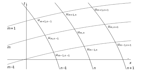
Figure 1: Example of a two-dimensional lattice.

The discrete jet space will be the set of all variables $\{x_{jk},t_{jk},u_{jk}\}$ on the lattice. The dependence of $x$, $t$ and $u$ on the labels $m$, $n$ is determined from the difference system

$$\mathcal{E}_{mn}^{a}(x_{jk},t_{jk},u_{jk})=0,\quad a=1,\cdots,N,$$ (12)

and some boundary conditions. In eq. (12) $N$ is an integer satisfying $N\geq 3$ and $(j,k)$ run over some finite set of values on the lattice while $(m,n)$ is a fixed reference point. Eq. (12) thus determines both the difference equation and the lattice.

Lie point symmetries of the system (12) are generated by vector fields of the form

$$\hat{X}_{mn}^{D}=\xi(x_{mn},t_{mn},u_{mn})\partial_{x_{mn}}+\tau(x_{mn},t_{mn},u_{mn})\partial_{t_{mn}}+\phi(x_{mn},t_{mn},u_{mn})\partial_{u_{mn}}$$ (13)

(the superscript $D$ stands for ‘discrete‘) satisfying

$$\mbox{pr}\hat{X}^{D}\mathcal{E}^{a}|_{\mathcal{E}^{1}=\mathcal{E}^{2}=\cdots=\mathcal{E}^{N}=0}=0.$$ (14)

In eq. (14) $\mbox{pr}\hat{X}^{D}$ is the prolongation of the vector field $\hat{X}_{mn}^{D}$ to the discrete jet space

$$\mbox{pr}\hat{X}^{D}=\sum_{j,k}\hat{X}_{jk}^{D},$$ (15)

where the sum is over all points figuring in the difference system (12).

In this approach the lattice $(x_{mn},t_{mn})$ is in general determined together with $u_{mn}$ from the system (12) and the group transformations generated by the vector field $\hat{X}_{mn}^{D}$ also transform the lattice. A special case corresponds to an a priori determined nontransforming lattice. In that case two of the equations in the system (12) have the form

$$x_{mn}=f(m,n),\qquad t_{mn}=g(m,n),$$ (16)

where $f$ and $g$ are given. Such is the case of a uniform orthogonal lattice where (16) takes the form

$$x_{mn}=\sigma_{1}n+x_{0},\qquad t_{mn}=\sigma_{2}m+t_{0},$$ (17)

and the scale factors $(\sigma_{1},\sigma_{2})$ and the origin $(x_{0},t_{0})$ are given numbers (e.g. $\sigma_{1}=\sigma_{2}=1,\,x_{0}=t_{0}=0)$.

We are interested in obtaining the form of the vector field in the semicontinuous limit in which $t_{mn}$ becomes a continuous variable $t$, but $x_{mn}$ remains discrete ( and independent of $t$). Thus $x$ will depend on one discrete label $n$ only and in particular $x$ may be given as $x_{n}=f(n)$, with $f(n)$ known (e.g. $x_{n}=hn$ for a uniform lattice, or $x_{n}=\lambda^{n}$ for an exponential one).

In this limit the difference system (12) will reduce to a differential–difference equation (D$\Delta$E)

$$\mathcal{E}_{n}(t,u_{j},\dot{u}_{j},\ddot{u}_{j},\cdots,u_{j}^{(K)})=0,\quad n-L\leq j\leq n+M,$$ (18)

where dots denote $t$–derivatives, and $K$, $L$ and $M$ are some nonnegative integers. Together with eq. (18) we have another equation which determines $x_{n}=f(n)$. We shall consider the case when $f(n)$ is already given (a known function) so that we can replace the dependence on $x_{n}$ by a dependence on the integer $n$ (without necessarily assuming that $f(n)$ is linear).

Eq. (18) is thus defined on a ‘semidiscrete jet space‘ with local coordinates

$$\{t,u_{j},\dot{u}_{j},\ddot{u}_{j},\cdots,u_{j}^{(K)}\},$$ (19)

where $j$ runs over all values on a one–dimensional lattice.

The vector field generating symmetries of eq. (18) will have the form

$$\hat{X}^{SD}=\tau_{n}(t,u_{n})\partial_{t}+\phi_{n}(t,u_{n})\partial_{u_{n}},$$ (20)

($SD=$ semidiscrete) and its prolongation will be defined on the semidiscrete jet space (19).

Let us consider the simplest nontrivial case, namely that of a difference system (12) involving the three points $(m,n)$, $(m+1,n)$ and $(m,n+1)$, i.e. relating the variables $x_{jk}$, $t_{jk}$ and $u_{jk}$ in these 3 points:

$$\mathcal{E}_{n}(x_{mn},x_{m+1,n},x_{m,n+1},t_{mn},t_{m+1,n},t_{m,n+1},u_{mn},u_{m+1,n},u_{m,n+1})=0.$$ (21)

Before taking the limit we change notation and transform to new variables. We choose a reference point $(m,n)$ on the lattice (see Fig.1) and measure $t$ and $x$ from this point:

$$t_{m+a,n+b}=t+\epsilon_{ab},\quad x_{m+a,n+b}=f(n+b)+\theta(\epsilon_{ab}),$$ (22)

where $f(n+b)$ is a given function and $\theta(\epsilon_{ab})$ is an analytic function. Instead of $u_{m+j,n+k}$ we introduce a function $v_{n}(t)$

$$v_{n+b}(t+\epsilon_{ab})\equiv u_{m+a,n+b}(x_{m+a,n+b},t_{m+a,n+b}),$$ (23)

and assume that the dependence on $t$ is analytical. Thus the dependence on $x$ (which remains discrete in the limit $\epsilon_{ab}\rightarrow 0$) is replaced by a dependence on the label $n+b$. For the reference point $x_{mn}$, $t_{mn}$ we put $\epsilon_{00}=0$, $\theta(\epsilon_{00})=0$.

So, in the case of the stencil $(m,n)$, $(m+1,n)$ and $(m,n+1)$ we have

$$t_{mn}\equiv t,\qquad t_{m+1,n}\equiv t+\epsilon_{10},\qquad t_{m,n+1}\equiv t+\epsilon_{01},$$

$$x_{mn}\equiv f(n),\qquad x_{m+1,n}=f(n)+\theta(\epsilon_{10}),\qquad x_{m,n+1}\equiv f(n+1)+\theta(\epsilon_{01}),$$

$$u_{mn}(x_{mn},t_{mn})=v_{n}(t),\qquad u_{m+1,n}\equiv v_{n}(t)+\epsilon_{10}v_{n,t}(t),$$ (24)

$$u_{m,n+1}(x_{m,n+1},t_{m,n+1})=v_{n+1}(t+\epsilon_{01})=v_{n+1}(t)+\sum_{j=1}^{\infty}\frac{\epsilon_{01}^{j}}{j!}v_{n+1}^{(j)}(t),$$

where $v_{n+1}^{(j)}(t)=\frac{d^{j}v_{n+1}(t)}{dt^{j}}$ and $v_{n,t}$ is the ‘discrete derivative‘ of $v_{n}(t)$ given by $v_{n}(t)=\frac{u_{m+1,n}-u_{m,n}}{\epsilon_{10}}$.

Since $v_{n}(t)$ is by assumption analytical, the Taylor series in (24) are convergent. Using eq. (24) we can also express the derivatives $\{\partial_{t_{mn}}$, $\partial_{t_{m+1,n}}$, $\partial_{t_{m,n+1}}$, $\partial_{u_{mn}}$, $\partial_{u_{m+1,n}}$, $\partial_{u_{m,n+1}}\}$ in terms of $\{\partial_{t}$, $\partial_{\epsilon_{10}}$, $\partial_{\epsilon_{01}}$, $\partial_{v_{n}}$, $\partial_{v_{n,t}}$, $\partial_{v_{n+1}}\}$ and thus transform the prolongation of the vector field (15). We obtain

$$\mbox{pr}\hat{X}^{D} = \tau_{mn}\partial_{t}+\phi_{mn}\partial_{v_{n}}+(\tau_{m+1,n}-\tau_{mn})\partial_{\epsilon_{10}}+(\tau_{m,n+1}-\tau_{mn})\partial_{\epsilon_{01}}$$

$$+ \Bigl{[}(\phi_{m+1,n}-\phi_{mn})+(\tau_{mn}-\tau_{m+1,n})v_{n,t}\Bigr{]}\frac{1}{\epsilon_{10}}\partial_{v_{n,t}}$$

$$+ \Bigl{[}\phi_{m,n+1}+(\tau_{mn}-\tau_{m,n+1})\sum_{j=1}^{\infty}\frac{(t_{m,n+1}-t_{mn})^{j-1}}{(j-1)!}v_{n+1}^{(j)}\Bigr{]}\partial_{v_{n+1}}.$$

Further, we put

$$\tau_{mn}\equiv\tau_{n}(t,v_{n}),\qquad\phi_{mn}\equiv\phi_{n}(t,v_{n}),$$ (26)

and expand $\tau_{m+1,n}$ and $\phi_{m+1,n}$ about $\epsilon_{10}=0$, $\tau_{m,n+1}$ and $\tau_{m,n+1}$ and $\phi_{m,n+1}$ about $\epsilon_{01}=0$ and then let $\mbox{pr}\hat{X}^{D}$ act on functions

$$\mathcal{E}_{n}=\mathcal{E}_{n}(t,v_{n},v_{n+1},v_{n,t}),$$ (27)

obtained as the limit of eq. (21). In the semicontinuous limit we take $\epsilon_{10}\rightarrow 0$, $\epsilon_{01}\rightarrow 0$ and we obtain

$$\lim_{(\epsilon_{10},\epsilon_{01})\rightarrow(0,0)}\mbox{pr}\hat{X}^{D} = \mbox{pr}\hat{X}^{SD}=\tau_{n}\partial_{t}+\phi_{n}\partial_{v_{n}}+\phi_{n}^{[t]}\partial_{v_{n,t}}+\phi_{n}^{[n+1]}\partial_{v_{n+1}^{(1)}},$$ (28)

$$\phi_{n}^{[t]} = D_{t}\phi_{n}-(D_{t}\tau_{n})\dot{v}_{n},$$ (29)

$$\phi_{n}^{[n+1]} = \phi_{n+1}+(\tau_{n}-\tau_{n+1})v_{n+1}^{(1)}.$$ (30)

The form (29) of the coefficient $\phi_{n}^{[t]}$ is the ”obvious” generalization of the first prolongation for ordinary differential equations. The presence of the second term in (30) is less obvious and follows from the above analysis of the semicontinuous limit. We see that the prolongation of the vector field $\hat{X}^{SD}$ to derivatives is the same as for differential equations The prolongation to other points $x_{n}$ on the lattice does however not consist of merely shifting $n$ in $\phi_{n}$.

We mention that the additional term in $\phi_{n}^{[n+1]}$ was missed in the article [9].

If we start from the set of all 9 points on the stencil of Fig.1 and take the semicontinuous limit in the same way, we arrive at a more general D$\Delta$E, namely

$$\mathcal{E}_{n}(t,u_{n},u_{n+1},u_{n-1},\dot{u}_{n},\dot{u}_{n+1},\dot{u}_{n-1},\ddot{u}_{n},\ddot{u}_{n+1},\ddot{u}_{n-1})=0,$$ (31)

(with the change of notation to $u_{n}$). We also obtain the prolongation $\mbox{pr}\hat{X}^{SD}$ for such an equation (see below).

2.2 The Evolutionary Formalism and Commuting Flows for Differential–Difference Equations

An alternative method of calculating symmetries of D$\Delta$E on a fixed lattice is to construct commuting flows in two variables. Let us again consider eq. (27), this time solved for the first derivative, and change the notation from $\dot{v}_{n}$ to $u_{n,t}$, which now denotes an ordinary time derivative;

$$\dot{u}_{n}\equiv u_{n,t}=\mathcal{F}_{n}(t,u_{n},u_{n+1}).$$ (32)

We introduce an additional variable $\lambda$, the group parameter and consider the flow on $u_{n}(t,\lambda)$ in this variable

$$u_{n,\lambda}=\mathcal{Q}_{n}(t,u_{n},\dot{u}_{n}).$$ (33)

Let us now require that the flows (32) and (33) be compatible, i.e. commute. Thus we impose

$$u_{n,t\lambda}=u_{n,\lambda t}.$$ (34)

We replace $u_{n,\lambda}$ using eq. (33), $\dot{u}_{n}$ and $\ddot{u}_{n}$ using (32) and its differential consequences and obtain

$$\mathcal{Q}_{n,t} + \mathcal{Q}_{n,u_{n}}\mathcal{F}_{n}+\mathcal{Q}_{n,\dot{u}_{n}}\bigl{(}\mathcal{F}_{n,t}+\mathcal{F}_{n,u_{n}}\mathcal{F}_{n}+\mathcal{F}_{n,u_{n+1}}\mathcal{F}_{n+1}\bigr{)}=$$

$$\mathcal{F}_{n,u_{n}}\mathcal{Q}_{n}+\mathcal{F}_{n,u_{n+1}}\mathcal{Q}_{n+1}.$$

This derivation of (2.2)is completely equivalent to the following procedure. We first introduce an evolutionary vector field

$$\hat{X}_{E}=\mathcal{Q}_{n}(t,u_{n},\dot{u}_{n},\cdots)\partial_{u_{n}},$$ (36)

and its prolongation

$$\mbox{pr}\hat{X}_{E}=\mathcal{Q}_{n}\partial_{u_{n}}+\mathcal{Q}_{n+1}\partial_{u_{n+1}}+(D_{t}\mathcal{Q}_{n})\partial_{\dot{u}_{n}}+\cdots.$$ (37)

We then apply this prolonged field to eq. (32), require

$$\mbox{pr}\hat{X}_{E}\bigl{[}\dot{u}_{n}-\mathcal{F}_{n}(t,u_{n},u_{n+1})\bigr{]}\Bigl{|}_{(\dot{u}_{n}=\mathcal{F}_{n},\ddot{u}_{n}=D_{t}\mathcal{F}_{n})}=0,$$ (38)

and reobtain eq. (2.2).

Let us now specialize to the case of point symmetries. The quantity $\mathcal{Q}_{n}$ in (33) and (36) is the characteristic of the vector field $\hat{X}_{E}$. For point symmetries it has the form

$$\mathcal{Q}_{n}(t,u_{n},\dot{u}_{n},\cdots)=\phi_{n}(t,u_{n})-\tau_{n}(t,u_{n})\dot{u}_{n}.$$ (39)

The total derivative $D_{t}$ is itself a (generalized) symmetry of the D$\Delta$E (18) and in particular (32). This provides us with a relation between ordinary and evolutionary vector fields and their prolongations, namely

$$\mbox{pr}\hat{X}=\mbox{pr}\hat{X}_{E}+\tau_{n}(t,u_{n})D_{t}.$$ (40)

Putting (39) and (37) into (40) we reobtain eqs. (28–30).

We see that the ”obvious” prolongation (37)of the evolutionary vector field (36) provides, via eq. (40) the correct prolongation (28) of the ordinary vector field (20).

2.3 General Algorithm for Calculating Lie Point Symmetries of a Differential Difference Equation

Let us consider a D$\Delta$E involving $L+M+1$ points and $t$ derivatives up to order $K$ as in eq. (18). The Lie point symmetries of eq. (18) can be obtained using the evolutionary formalism by imposing

$$\mbox{pr}\hat{X}_{E}\mathcal{E}_{n}\bigl{|}_{\mathcal{E}_{n}=0,\,D^{k}_{t}\mathcal{E}_{n}=0}=0,\qquad k=1,\cdots,K.$$ (41)

Thus the expression $\mbox{pr}\hat{X}_{E}\mathcal{E}_{n}$ is anihilated on the solution set of the equation (18) and of all differential consequences of the equation.

The vector field $\hat{X}_{E}$ has the form (36) with $\mathcal{Q}_{n}$ as in (39). The prolongation of $\hat{X}_{E}$ is

$$\mbox{pr}\hat{X}_{E}=\sum_{j}\mathcal{Q}_{j}\partial_{u_{j}}+\sum_{k=1}^{K}\sum_{j`}(D_{t}^{k}\mathcal{Q}_{j})\partial_{u_{j}^{(k)}},$$ (42)

where the $j$ summation is over all points figuring in eq. (18) and $u_{j}^{(k)}$ denotes the $k$–th $t$–derivative of $u_{j}$.

The standard vector field $\hat{X}$ generating Lie point symmetries and its prolongation are given by the formula (40). Explicitly the prolongation formula is

$$\mbox{pr}\hat{X} = \phi_{n}\partial_{u_{n}}+\tau_{n}\partial_{t}+\sum_{j\neq n}\phi_{j}\partial_{u_{j}}$$

$$+ \sum_{j}\sum_{k=1}^{K}\phi_{j}^{[k]}\partial_{u_{j}^{[k]}}+\sum_{j}\sum_{k=1}^{K}(\tau_{n}-\tau_{j})(D_{t}^{k+1}u_{j})\partial_{u_{j}^{[k]}},$$

$$\phi_{j}^{[k]} = D_{t}\phi_{j}^{[k-1]}-(D_{t}\tau_{j})u_{j}^{[k]},\qquad D_{t}^{k}u_{j}\equiv u_{j}^{[k]}.$$ (44)

Notice that $\phi_{j}^{[k]}$ is the same as for a differential equation [18] but the last term in (2.3) has no analog in the continuous case. The coefficients $\phi_{n}$ and $\tau_{n}$ in the vector field $\hat{X}$ itself are a priori functions of $n$, $t$ and $u_{n}$ (see eq. (20)). In the following section we will examine some cases when $\tau_{n}(t,u_{n})$ simplifies.

Eq. (2.3) is also obtained as the semicontinuous limit of the discrete prolongation (15)

3 Theorems Simplifying the Calculation of Symmetries of D$\Delta$E.

3.1 General comments

Lie point symmetries of D$\Delta$E of the form (18) are generated by vector fields of the form (20). We shall now investigate 3 important cases when the coefficient $\tau_{n}(t,u_{n})$ actually depends on $t$ alone.

The 3 classes of D$\Delta$E are

$$\dot{u}_{n}= f_{n}(t,u_{n-1},u_{n},u_{n+1}),$$ (45)

$$\ddot{u}_{n}= f_{n}(t,\dot{u}_{n},u_{n-1},u_{n},u_{n+1}),$$ (46)

$$u_{n,xy}= f_{n}(x,y,u_{n,x},u_{n,y},u_{n-1},u_{n},u_{n+1}).$$ (47)

Eq. (45) contains integrable Volterra, modified Volterra and discrete Burgers type equations [23]. A list of integrable Toda type equations of the form (46) can be found in the reference [24]. The class (47) involves 2 continuous variables and contains the two dimensional Toda model [14, 4]. A list of integrable cases exists [19] and Lie point symmetries of this class have been studied.

For equations (45) and (46) Lie point symmetries correspond to commuting flows of the form (33) with $\mathcal{Q}_{n}$ given by eq. (39) while for eq. (47) the form is

$$u_{n,\lambda}=\psi_{n}(x,y,u_{n},u_{n,x},u_{n,y}),$$ (48a)

$$\psi_{n}(x,y,u_{n},u_{n,x},u_{n,y})=\phi_{n}(x,y,u_{n})-\xi_{n}(x,y,u_{n})u_{n,x}-\eta_{n}(x,y,u_{n})u_{n,y}.$$ (48b)

For all equations (45, 46, 47), we assume everywhere below that at least one of the following two conditions is satisfied:

$$\frac{\partial f_{n}}{\partial u_{n+1}}\neq 0,\quad\hbox{for all}\ n,\qquad\mbox{or}\qquad\frac{\partial f_{n}}{\partial u_{n-1}}\neq 0,\quad\hbox{for all}\ n.$$ (49)

3.2 Volterra type equations and their generalizations.

Let us consider eq. (45).

Theorem 3.1.

If (45) satisfies at least one of the conditions (49) and (33) represents a point symmetry of (45) then we have

$$\tau_{n}(t,u_{n})=\tau(t).$$ (50)

Proof.

The compatibility condition (34) of eqs. (45) and (33, 39) implies

$$\sum_{l=-1}^{1}f_{n,u_{n+l}}[\phi_{n+l}-\tau_{n+l}f_{n+l}]+(\tau_{n,t}+\tau_{n,u_{n}}f_{n})f_{n}+$$ (51)

$$+\tau_{n}[f_{n,t}+\sum_{l=-1}^{1}f_{n,u_{n+l}}f_{n+l}]-\phi_{n,t}-\phi_{n,u_{n}}f_{n}=0,$$

where indices $t$, $u_{n+l}$ denote partial derivatives. Taking the derivative of eq. (51) with respect to $u_{n+2}$ and separately with respect to $u_{n-2}$, we obtain two relations:

$$f_{n+1,u_{n+2}}f_{n,u_{n+1}}(\tau_{n}-\tau_{n+1})=0,$$ (52)

$$f_{n-1,u_{n-2}}f_{n,u_{n-1}}(\tau_{n}-\tau_{n-1})=0.$$

In view of the conditions (49), eqs. (52) imply

$$\tau_{n+1}(t,u_{n+1})=\tau_{n}(t,u_{n})\quad\hbox{or}\quad\tau_{n-1}(t,u_{n-1})=\tau_{n}(t,u_{n}).$$ (53)

Each of these conditions must be satisfied for any $n$ and they are equivalent. Since $u_{0},u_{1},u_{-1},\dots$ are independent, we find that $\tau_{n}(t,u_{n})$ depends on $t$ alone and this proves Theorem 3.1.  

A somewhat weaker theorem can be proved for a more general differential–difference equation, namely,

$$\dot{u}_{n}=f_{n}(t,u_{n+k},u_{n+k+1},\cdots,u_{n+m}),\quad k\leq m.$$ (54)

Theorem 3.2.

Let Eqs. (33, 39) represent a symmetry of eq. (54). If the function $f_{n}$ in (54) satisfies

$$m>0,\qquad\frac{\partial f_{n}}{\partial u_{n+m}}\neq 0\quad\hbox{for all}\ n,$$ (55)

then the function $\tau_{n}(t,u_{n})$ is such that

$$\tau_{n}(t,u_{n})=\tau_{n}(t),\qquad\tau_{n+m}(t)=\tau_{n}(t).$$ (56)

If the function $f_{n}$ satisfies

$$k<0,\qquad\frac{\partial f_{n}}{\partial u_{n+k}}\neq 0\quad\hbox{for all}\ n,$$ (57)

then we have

$$\tau_{n}(t,u_{n})=\tau_{n}(t),\qquad\tau_{n+k}(t)=\tau_{n}(t).$$ (58)

Proof.

The compatibility condition for Eqs.(33, 39) and (54) will be the same as Eq. (51) but all sums will be from $l=k$ to $l=m$. If Eq. (55) is satisfied we can differentiate eq. (51) with respect to $u_{n+2m}$ and obtain $\tau_{n}(t,u_{n})=\tau_{n+m}(t,u_{n+m})$ which implies (56). If (57) is satisfied we differentiate (51) with respect to $u_{n+2k}$ and obtain $\tau_{n}(t,u_{n})=\tau_{n+k}(t,u_{n+k})$ which implies (58).  

This result is valid, in particular, for Burgers type equations for which $k=0$, $m>0$ or $k<0$, $m=0$ For all equations in the class (54), under the assumptions of this theorem, the function $\tau_{n}$ is independent of $u_{n}$ and is periodic in $n$. In particular, if $k=-2$, $m=2$ it is two-periodic and we can write

$$\tau_{n}(t)=\frac{1+(-1)^{n}}{2}\tau_{0}(t)+\frac{1-(-1)^{n}}{2}\tau_{1}(t).$$ (59)

3.3 Toda type equations

The compatibility condition for eq. (46) and Eqs. (33, 39) is $u_{n,tt\lambda}=u_{n,\lambda tt}$ and implies

$$f_{n,\dot{u}_{n}}[\phi_{n,t}+(\phi_{n,u_{n}}-\tau_{n,t})\dot{u}_{n}-\tau_{n,u_{n}}(\dot{u}_{n})^{2}]$$ (60)

$$+\sum_{k=-1}^{1}f_{n,u_{n+k}}[\phi_{n+k}+(\tau_{n}-\tau_{n+k})\dot{u}_{n+k}]$$

$$-\phi_{n,tt}+(-2\phi_{n,tu_{n}}+\tau_{n,tt})\dot{u}_{n}+(-\phi_{n,u_{n}u_{n}}+2\tau_{n,tu_{n}})(\dot{u}_{n})^{2}$$

$$+\tau_{n,u_{n}u_{n}}(\dot{u}_{n})^{3}+\tau_{n}f_{n,t}+(2\tau_{n,t}-\phi_{n,u_{n}}+3\tau_{n,u_{n}}\dot{u}_{n})f_{n}=0.$$

We use Eq. (60) to prove the following theorem.

Theorem 3.3.

Let Eqs. (33, 39) represent a point symmetry of Eq. (46) and let the function $f_{n}$ in Eq. (46) satisfy at least one of the conditions (49) for all $n$. Then the function $\tau_{n}(t,u_{n})$ in eq. (39) satisfies Eq. (50), i.e. $\tau_{n}(t,u_{n})$ depends on $t$ alone.

Proof.

None of the functions $f_{n}$, $\phi_{n}$, $\tau_{n}$ figuring in eq. (60) depends on $\dot{u}_{n+1}$ or $\dot{u}_{n-1}$. These two expressions do however figure explicitly in (60). Their coefficients must hence vanish and we obtain

$$f_{n,u_{n+1}}(\tau_{n}-\tau_{n+1})=0,$$ (61)

$$f_{n,u_{n-1}}(\tau_{n}-\tau_{n-1})=0.$$

In view of the conditions (49), we can use one of eqs. (61), and both of them provide the same:

$$\tau_{n}(t,u_{n})=\tau_{n+1}(t,u_{n+1})$$ (62)

for any $n$. Hence we again obtain the result (50), as stated in Theorem 3.3.  

3.4 Toda field theory type equations

Let us now consider the equation (47) and assume that it has a Lie point symmetry represented by (48).

Theorem 3.4.

Let (48) represent a Lie point symmetry of the field equation (47) and let the function $f_{n}(x,y,u_{n,x},u_{n,y},u_{n-1},u_{n},u_{n+1})$ satisfy at least one of the conditions

$$\frac{\partial f_{n}}{\partial u_{n-1}}\neq 0,\quad\mbox{or}\quad\frac{\partial f_{n}}{\partial u_{n+1}}\neq 0.$$ (63)

The functions $\xi_{n}$ and $\eta_{n}$ in the symmetry (48) then are given by

$$\xi_{n}(x,y,u_{n})=\xi(x,y),\qquad\eta_{n}(x,y,u_{n})=\eta(x,y).$$ (64)

Proof.

The compatibility condition $u_{n,xy\lambda}=u_{n,\lambda xy}$ in this case can be written as

$$\sum_{k=-1}^{1}\frac{\partial f_{n}}{\partial u_{n+k}}\psi_{n+k}+\frac{\partial f_{n}}{\partial u_{n,x}}D_{x}\psi_{n}+\frac{\partial f_{n}}{\partial u_{n,y}}D_{y}\psi_{n}-D_{x}D_{y}\psi_{n}=0$$ (65)

with $\psi_{n}$ as in Eq. (48b); $D_{x}$ and $D_{y}$ are the total derivative operators. The terms $u_{n\pm 1,x}$, $u_{n\pm 1,y}$ only figure in $\psi_{n\pm 1}$ and in $D_{x}D_{y}\psi_{n}$ where we have

$$D_{x}D_{y}\psi_{n}=-\xi_{n}(D_{x}f_{n})-\eta_{n}(D_{y}f_{n})+\cdots$$

with

$$D_{x}f_{n}=\frac{\partial f_{n}}{\partial u_{n-1}}u_{n-1,x}+\frac{\partial f_{n}}{\partial u_{n+1}}u_{n+1,x}+\cdots$$

$$D_{y}f_{n}=\frac{\partial f_{n}}{\partial u_{n-1}}u_{n-1,y}+\frac{\partial f_{n}}{\partial u_{n+1}}u_{n+1,y}+\cdots.$$

Substituting into (65) and setting the coefficients of $u_{n\pm 1,x}$ and $u_{n\pm 1,y}$ equal to zero separately, we obtain

$$(\xi_{n-1}-\xi_{n})\frac{\partial f_{n}}{\partial u_{n-1}}=0,\quad (\eta_{n-1}-\eta_{n})\frac{\partial f_{n}}{\partial u_{n-1}}=0,$$

$$(\xi_{n+1}-\xi_{n})\frac{\partial f_{n}}{\partial u_{n+1}}=0,\quad (\eta_{n+1}-\eta_{n})\frac{\partial f_{n}}{\partial u_{n+1}}=0.$$

Thus, under the assumption (63) we obtain (64) and this completes the proof.    

4 Examples

Let us now consider examples of each of the classes of differential–difference equations discussed in Section 3.

4.1 The YdKN equation

The Krichever–Novikov equation [5]

$$\dot{u}=\frac{1}{4}u_{xxx}-\frac{3}{8}\frac{u_{xx}^{2}}{u_{x}}+\frac{3}{2}\frac{P(u)}{u_{x}},$$ (67)

where $P(u)$ is an arbitrary fourth degree polynomial with constant coefficients, is an integrable PDE with many interesting properties [5, 17, 3, 8, 6, 15, 16, 20, 7, 21, 1].

Yamilov and collaborators have proposed integrable discretizations of eq. (67) [13, 23, 25]. The original form of the YdKN equation [23, 25] is

$$u_{n,t} = \frac{P_{n}u_{n+1}u_{n-1}+Q_{n}(u_{n+1}+u_{n-1})+R_{n}}{u_{n+1}-u_{n-1}},$$ (68)

$$P_{n} = \alpha u_{n}^{2}+2\beta u_{n}+\gamma,$$ (69)

$$Q_{n} = \beta u_{n}^{2}+\lambda u_{n}+\delta,$$

$$R_{n} = \gamma u_{n}^{2}+2\delta u_{n}+\omega,$$

where $\alpha,\cdots,\omega$ are pure constants.

A complete symmetry analysis of this equation and its generalizations is in preparation [12]. Here we will just consider one special case as an example of a Volterra type equation. Let us set $\alpha=1$, $\beta=\cdots=\omega=0$ in (69). The YdKN equation reduces to

$$u_{n,t}=\frac{u_{n}^{2}u_{n+1}u_{n-1}}{u_{n+1}-u_{n-1}}.$$ (70)

According to Theorem 3.1 a compatible flow corresponding to a point symmetry will have the form

$$u_{n,\lambda}=\Phi_{n}(t,u_{n})-\tau(t)u_{n,t}.$$ (71)

We replace $u_{n,t}$ in (71) using (70) and then impose the compatibility condition $u_{n,t\lambda}=u_{n,\lambda t}$. First of all, from terms containing $u_{n+2}$ and $u_{n-2}$ we find that $\Phi_{n}$ and $\tau$ must satisfy

$$\tau =\tau_{0}+\tau_{1}t,\quad\Phi_{n} =a_{n}+b_{n}u_{n}+c_{n}u_{n}^{2},$$ (72)

$$a_{n} =a+\hat{a}(-1)^{n},\quad b_{n} =b+\hat{b}(-1)^{n},\quad c_{n}=c+\hat{c}(-1)^{n},$$

where $\tau_{0},\tau_{1},a,\hat{a},b,\hat{b},$ and $c,\hat{c}$ are pure constants. This is actually the case for the general YdKN equation (68). Substituting (72) into the compatibility condition we obtain an equation that is polynomial in $u_{n+k}$. Setting coefficients of $u_{n-1}^{a}u_{n}^{b}u_{n+1}^{c}$ equal to zero for each independent term we obtain the following basis of the Lie point symmetry algebra of eq. (70)

$$X_{1} = \partial_{t},\quad X_{2}=u_{n}^{2}\partial_{u_{n}},\quad X_{3}=(-1)^{n}u_{n}^{2}\partial_{u_{n}},$$ (73)

$$X_{4} = t\partial_{t}-\frac{1}{2}u_{n}\partial_{u_{n}},\qquad X_{5}=(-1)^{n}u_{n}\partial_{u_{n}}.$$

This is a solvable Lie algebra with $\{X_{1},X_{2},X_{3}\}$its Abelian niilradical. The two nonnilpotent elements satisfy $[X_{4},X_{5}]=0$ and their action on the nilradical is given by

$$\left(\begin{array}[]{c}{[X_{4},X_{1}]}\\ {[X_{4},X_{2}]}\\ {[X_{4},X_{3}]}\end{array}\right) = \left(\begin{array}[]{ccc}-1&0&0\\ 0&-\frac{1}{2}&0\\ 0&0&-\frac{1}{2}\end{array}\right)\left(\begin{array}[]{c}X_{1}\\ X_{2}\\ X_{3}\end{array}\right),$$ (83)

$$\left(\begin{array}[]{c}{[X_{5},X_{1}]}\\ {[X_{5},X_{2}]}\\ {[X_{5},X_{3}]}\end{array}\right) = \left(\begin{array}[]{ccc}0&0&0\\ 0&0&1\\ 0&1&0\end{array}\right)\left(\begin{array}[]{c}X_{1}\\ X_{2}\\ X_{3}\end{array}\right).$$ (93)

4.2 The Toda lattice

The Toda lattice itself

$$u_{n,tt}=\exp(u_{n-1}-u_{n})-\exp(u_{n}-u_{n+1}),$$ (94)

is the best known example of an equation of the type (46). According to Theorem 3.3 the flow corresponding to its point symmetries will satisfy (71). From the compatibility condition $u_{n,tt\lambda}=u_{n,\lambda tt}$ we obtain the Lie point symmetry algebra

$$X_{1}=\partial_{t},\quad X_{2}=t\partial_{u_{n}},\quad X_{3}=\partial_{u_{n}},\quad X_{4}=t\partial_{t}+2n\partial_{u_{n}}.$$ (95)

This Lie algebra is solvable, its nilradical $\{X_{1},X_{2},X_{3}\}$ is isomorphic to the Heisenberg algebra. We note that the Ansatz made in [9] was not correct and lead to $X_{3}=q(n)\partial_{u_{n}}$ in (95) with $q(n)$ arbitrary. It was however noted there that a closed Lie algebra is obtained only for $q(n)=\mbox{const}$.

4.3 The two–dimensional Toda lattice equation.

The equation to be considered [4, 14] is

$$u_{n,xy}=\exp(u_{n-1}-u_{n})-\exp(u_{n}-u_{n+1}).$$ (96)

According to Teorem 3.4 the flow corresponding to point symmetries will take the form

$$u_{n,\lambda}=\phi_{n}(x,y,u_{n})-\xi(x,y)u_{n,x}-\eta(x,y)u_{n,y}.$$ (97)

The Lie point symmetry algebra obtained from the compatibility condition $u_{n,xy\lambda}=u_{n,\lambda xy}$ is infinite–dimensional and depends on 4 arbitrary function of one variable each

$$X(f) = f(x)\partial_{x}+f^{\prime}(x)n\partial_{u_{n}},\quad U(k)=k(x)\partial_{u_{n}},$$ (98)

$$X(g) = g(y)\partial_{y}+g^{\prime}(y)n\partial_{u_{n}},\quad W(\ell)=\ell(y)\partial_{u_{n}}.$$

This algebra happens to coincide with the one found in [10] through the prolongation formula used there was incorrect. This is a Kac–Moody–Virasoro algebra as is typical for integrable equations with more than 2 independent variables (in this case $x,y$ and $n$).

5 Conclusions

The main results of the present article are:

1. The prolongation formulas (41) and (42), (2.3) for evolutionary and ordinary vector fields generating commuting flows and Lie point symmetry transformation for differential–difference equations. These are viewed here as differential equations on fixed non–transforming lattices.

2. The prolongation formulas and the corresponding algorithm for calculating Lie point symmetries of differential–difference equations are greatly simplified for 3 rather general classes of equations ( including the Toda lattice, the two–dimensional Toda lattice and the Volterra equations). The results are summed up in Theorems 3.1–3.4.

3. We have presented an example of each class of equations covered by the above Theorems and identified a class of equations depending on 6 parameters (with generalizations depending on 9 parameters). These are the Yamilov discretizations of the Krichever–Novikov equation (68, 69).

A complete analysis of the symmetries of the YdKN equation and its generalizations will be published separately.

Acknowledgments.

RIY has been partially supported by the Russian Foundation for Basic Research (grant numbers 08-01-00440-a and 09-01-92431-KE-a). The research of P.W. was partially supported by a research grant from NSERC of Canada. LD has been partly supported by the Italian Ministry of Education and Research, PRIN ”Nonlinear waves: integrable fine dimensional reductions and discretizations” from 2007 to 2009 and PRIN ”Continuous and discrete nonlinear integrable evolutions: from water waves to symplectic maps” from 2010.

References

• [1] V.E. Adler, A.B. Shabat and R.I. Yamilov, Symmetry approach to the integrability problem, Teoret. Mat. Fiz. 125 (2000), no. 3, 355–424 (in Russian); English translation in Theor. Math. Phys. 125 (2000), no. 3, 1603–1661.
• [2] V.A. Dorodnitsyn The Group Properties of Difference Equations (Moscow, Fizmatlit, 2001) (in Russian).
• [3] B. Dubrovin, I. Krichever, and S. Novikov, ”Integrable systems. I,” in: Itogi Nauki i Tekhn. Ser.: Sovr. Probl. Matem. [in Russian] (R. V. Gamkrelidze, ed.), Vol. 4, Dynamic Systems-4, VINITI, Moscow (1985), pp. 179-285.
• [4] A.P. Fordy and J. Gibbons Integrable nonlinear Klein–Gordon equations and Toda lattices Comm. Math. Phys. 71 (1980) 21–30.
• [5] 1. I. M. Krichever and S. P. Novikov,Holomorphic bundles and nonlinear equations. Finite-gap solutions of rank $2$, Sov. Math. Dokl. 20 (1979) 650-654.
• [6] I.M. Krichever and S.P. Novikov, Holomorphic bundles over algebraic curves and non-linear equations, Uspekhi Mat. Nauk 35 (1980), 47–68 (in Russian); English translation in Russ. Math. Surv. 35 (1980), 53–80.
• [7] G. Latham and E. Previato,Darboux transformations for higher-rank Kadomtsev-Petviashvili and Krichever-Novikov equations. Acta Appl. Math., 39 (1995) 405-433.
• [8] D. Levi, M. Petrera, C. Scimiterna and R. Yamilov, On Miura transformations and Volterra-type equations associated with the Adler-Bobenko-Suris equations, SIGMA 4 (2008), 077, 14 pages.
• [9] D. Levi and P. Winternitz, Continuous symmetries of discrete equations. Phys. Lett. A 152 (1991) 335–338.
• [10] D. Levi and P. Winternitz, Symmetries and conditional symmetries of differential-difference equations. J. Math. Phys. 34 (1993) 3713–3730.
• [11] D. Levi and P. Winternitz, Continuous symmetries of difference equations, J. Phys. A: Math. Gen. 39 (2006) R1 -R63.
• [12] D. Levi, P. Winternitz and R. Yamilov, Point Symmetries of the Yamilov Discretization of the Krichever-Novikov Equation and its Generalizations in preparation.
• [13] D. Levi and R. Yamilov, Conditions for the existence of higher symmetries of evolutionary equations on the lattice, J. Math. Phys. 38 (1997), 6648–6674.
• [14] A.V. Mikhailov, Integrability of two dimensional Toda chain Sov. Phys. JETP Lett. 30 (1979) 414–418.
• [15] O. I. Mokhov, Canonical Hamiltonian representation of the Krichever-Novikov equation, Math. Notes, 50, 939-945 (1991).
• [16] D. P. Novikov, Algebraic–geometric solutions of the Krichever–Novikov equation, Theoretical and Mathematical Physics, 121, 1999 1567–1573.
• [17] S. P. Novikov, S. V. Manakov, L. P. Pitaevsky, and V. E. Zakharov, Theory of Solitons: The Inverse Scattering Method [in Russian], Nauka, Moscow (1980); English transl., Plenum, New York (1984).
• [18] P.J. Olver Applications of Lie Groups to Difference Equations (New York, Springer 2000).
• [19] A.B. Shabat and R.I. Yamilov, To a transformation theory of two-dimensional integrable systems, Phys. Lett. A 227 (1997) 15–23.
• [20] V. V. Sokolov, Hamiltonian property of the Krichever– Novikov equation Sov. Math. Dokl., 30 (1984) 44-46.
• [21] S. I. Svinolupov, V. V. Sokolov, and R. I. Yamilov, Bäcklund transformations for integrable evolution equations. Sov. Math. Dokl., 28 (1983) 165-168.
• [22] P. Winternitz, Symmetries of Discrete Systems, Discrete Integrable Systems edited by B. Grammaticos, Y. Kosmann–Schwarzbach and T. Tamizhmani (Berlin, Springer, 2004) p. 185–243.
• [23] R.I. Yamilov, Classification of discrete evolution equations, Uspekhi Mat. Nauk 38 (1983), no. 6, 155–156 (in Russian).
• [24] R.I. Yamilov, Classification of Toda type scalar lattices, In: Proceedings of Int. Workshop NEEDS’92 (eds: V. Makhankov, I. Puzynin, O. Pashaev), World Scientific Publishing, 1993, 423–431.
• [25] R. Yamilov, Symmetries as integrability criteria for differential difference equations, J. Phys. A: Math. Gen. 39 (2006) R541–R623.