Resurvey of order and chaos in spinning compact binaries

Abstract

This paper is mainly devoted to applying the invariant fast Lyapunov indicator to clarify some doubt regarding the apparently conflicting results of chaos in spinning compact binaries at the second order post-Newtonian approximation of general relativity from previous literatures. It is shown with a number of examples that no single physical parameter or initial condition can be described as responsible for causing chaos, but a complicated combination of all parameters and initial conditions. In other words, a universal rule for the dependence of chaos on each parameter or initial condition cannot be found in general. For details, chaos does not depend only on the mass ratio, and the maximal spins do not necessarily bring the strongest effect of chaos. Additionally, chaos does not always become drastic when the initial spin vectors are nearly perpendicular to the orbital plane, and the alignment of spins cannot trigger chaos by itself alone.

I Introduction

Inspiralling compact binaries, made of neutron stars and/or black holes, are the most promising sources for gravitational-waves detectors such as LIGO and VIRGO. The successful analysis of the experimental data requires that signals should be drawn out of a lot of instrumental noise by matching observational data with a bank of theoretical templates. This is a match-filtering technique. However, the onset of chaos would make the implementation of this technique impractical. In this sense, the dynamical behavior of the system becomes a fascinating and interesting topic. There have been a number of articles in this field [1-13].

A point to deserve a little attention is that there are distinct results on chaos and order in spinning compact binaries in existing references [1,2,5,6,7,9,10,11]. These results seem to be cloudy and confusing, even apparently conflictive. They are originated from different approximations to the relativistic two-body problem, methods for diagnosing chaos, dynamical parameters and initial conditions. To clarify these doubt, we shall introduce more information for each case.

(i) Different equations of motion. A detailed discussion to the problem was given by Levin [12]. A conservative binary system composed of a nonspinning black hole and a spinning companion have three approximations: (1) the full relativistic system with the extreme-mass-ratio limit of a spinning particle orbiting a Schwarzschild black hole [1], (2) the post-Newtonian (PN) Lagrangian formulation with one body spinning [2,8], and (3) the PN Hamiltonian formulation with one body spinning [10,11]. Clearly, case (2) with case (3) just approaches to case (1) when the mass ratio becomes extreme. In spite of that, there are differently dynamical behaviors among the three approximations. The leading two approximations exhibit chaos [1,2], and the third does not at 2PN order [10,11]. As an illustration, chaos in case (1) happens only when the test particle around the Schwarzschild black hole has an unphysically large spin. For comparable mass binaries, either the Lagrangian formulation or the Hamiltonian formulation is often considered. It is worth emphasizing that the two approaches are only approximately equal, but not exactly. A typical difference between them lies in that the constants of motion are approximately accurate to some specific PN order for the former, while they are exactly conserved for the latter. Although there are such slight differences in the constants of motion between the two formulations, there is completely different dynamics in some sense. For instance, both the binary consisting of comparable-mass compact objects with one physically spinning body and the binary consisting of equal-mass compact objects with two arbitrary spins in the 2PN Lagrangian formulation do admit chaos [2,6-8], but their counterparts in the 2PN Hamiltonian formulation do not because they are actually integrable in the two simplified cases [10,11]. In all other situations, both the 2PN Lagrangian and the 2PN Hamiltonian favor the existence of chaos.

(ii) Indicators of chaos. There have been many methods to distinguish between ordered and chaotic motion. A Poincaré surface of section is easy to quantify chaos when the number of the dimension of phase space minus the number of all constants of motion is not more than three. The Poincaré surface is obtained by plotting a point in a certain two-dimensional (2D) plane of phase space each time when the orbit crosses a surface on which the other coordinates are fixed. A smooth curve, composed of the collection of points, represents the regular motion. On the other hand, the motion is chaotic if the points fill an area in this plane. However, this method of identifying chaos is less than ideal to describe the dynamics of a higher dimensional phase space. In this case, the largest Lyapunov exponent, as a measure of the average exponential deviation of two nearby orbits, is often used. In classical physics, there are two different techniques concerning its calculations. A rigorous method is called the variational method with a tangent vector, a solution of the variational equations [14]. It is necessary to rescale the size of the tangent vector from time to time so that overflows can be avoided. As an emphasis, it is cumbersome to derive the variational equations in general. In view of this factor, an alternative procedure to the variational method is to use the distance $d(t)$ at time $t$ in the phase space between two nearby trajectories as an approximation to the norm of the tangent vector. This approach is named as the two-particle method [14]. The method is valid if initial separation d(0) is sufficiently small and the renormalization is sufficiently frequent. By plotting $\ln\chi(t)$ vs $\ln t$ with $\chi(t)=(1/t)\ln[d(t)/d(0)]$, one can see that a negative constant slope signals the regularity of the orbit. If the slope tends gradually to zero, identically, $\ln\chi(t)$ arrives nearly at a certain stabilizing value, the bounded system turns out to be chaotic. This is practically attributed to a limit method for getting reliable Lyapunov exponents. On the other hand, there is a slightly different treatment by plotting $\ln[d(t)/d(0)]$ vs $t$ instead of $\ln\chi(t)$ vs $\ln t$. At once, $\chi$, as the slope of the fit line $\ln[d(t)/d(0)]=\chi t$, is the largest Lyapunov exponent. Here, it is necessary to perform a least-squares fit on the simulation data. This is a fit method. There should have been no difference in the computation of Lyapunov exponents between the fit method and the limit method, but it is easier and faster to get a fit slope than a stabilizing limit value [15]. It should be noted that a sufficiently long integration time is needed to get reliable Lyapunov exponents, especially for the limit method. Under this circumstance, a quicker and more sensitive indicator, the fast Lyapunov indicator of Froeschlé and Lega (FLI) [16], is recommended. This indicator means the natural logarithm of the length of a deviation vector, which stretches exponentially with time for a chaotic orbit but linearly for an ordered orbit. Thus, it allows one to distinguish between the ordered and chaotic cases. In addition, the frequency analysis method of Laskar [17] is much faster to detect chaos from regular than the method of the Lyapunov exponent. Of course, there are other equally fast, or faster methods to find chaos, for example, the method of the dynamical spectra of Voglis et al. [18], and the method of the smaller alignment index of Skokos [19]. For more information, see a comparison of the various methods in pages 277-280 of the book entitled “Order and Chaos in Dynamical Astronomy” by Contopoulos [20]. These methods, except the method of the Poincaré surface, are independent of the dimension of phase space.

General relativity has a time-redefinition ambiguity that allows any chaos apparently to be defined away by virtue of a spacetime coordinate transformation. There is a long history about the reliability of Lyapunov exponents in a curved space. A typical example is that Lyapunov exponents in the mixmaster cosmology depend on the choice of time variable [21-24]. Thus it is important enough to find a gauge invariant measure of chaos. Several independent groups have managed to work out this problem. Imponente & Montain [25] projected a geodesic deviation vector in the Jacobi metric on an orthogonal tetradic basis and obtained positive Lyapunov exponents of the mixmaster cosmology. So did Motter [26], who addressed directly the issue of the invariance of Lyapunov exponents. These invariant definitions of Lyapunov exponents are mainly focused on the time evolution of the gravitational field itself. On the other hand, for the geodesic or nongeodesic motion of particles in a given relativistic gravitational field, Wu & Huang [27] gave an invariant definition of Lyapunov exponents by refining the classical two-particle method. In their method, space projection operations are adopted, and coordinate time is chosen as an independent variable. This technique works well in the study of the chaotic dynamics in a superposed Weyl spacetime [28]. Wu et al. [29] introduced another invariant two-particle approach of Lyapunov exponents without projection operations and with proper time as the independent variable for a geodesic flow. If proper time and coordinate time do not satisfy an approximately logarithmic relation, the two kinds of invariant two-particle methods should be equivalent [29]. They also constructed the invariant FLI of two nearby trajectories. As to a spinning compact binary system with the PN equations of motion in coordinate time, it belongs to the nongeodesic case. By the 2PN bodies’ metrics in the center-of mass (CM) frame [30-33], one can easily note that the former invariant two-particle approach to Lyapunov exponents and its corresponding invariant FLI become possible applications in the dynamics of this system. Besides these invariant indicators, the fractal basin boundary method is regarded as to a coordinate invariant approach that gives a conclusion no ambiguity of spacetime coordinates. Although the system in the 2PN Lagrangian formulation is conservative, the coalescence of the black holes may occur. It should be emphasized that the coalescence is not a consequence of energy loss but just that these chaotic orbits happen to veer too close at some stage and merge. In this sense, the method of fractal basin boundaries is still a suitable tool. Usually, a basin is a 2D space $(\theta_{1},\theta_{2})$, where $\theta_{1}$ and $\theta_{2}$ are two initial spin angles. In this basin $\theta_{1}$ and $\theta_{2}$ are varied, and the other initial variables are fixed. As a result, one can determine whether the resulting orbits coalesce, escape to infinity, or remain stable and bounded. By color-coding each behavior and drawing points in the $(\theta_{1},\theta_{2})$ plane, one does observe the onset of chaos if the basin boundaries are fractal [2-4,6-8]. However, the fractal method has some limitations; for example, it makes no distinction between chaotic and ordered bound stable orbits in a non-fractal region of the basin, and gives no indication of the chaotic timescale either.

Now let us recall the existing references [2-8] on this chaos problem in the conservative 2PN Lagrangian formulation of spinning compact binaries by means of the related qualitative techniques above. Because of different methods adopted, there were initially some debates about the presence or absence of chaos in the system. With the help of the fractal basin boundary method, an earlier paper of Levin [2] depicted that spinning compact comparable mass binaries are shown to be chaotic in the PN expansion of the two-body system for some range of parameters. Furthermore, the authors of [5] employed the classical limit method to calculate Lyapunov exponents along the fractal of Ref. [2] and presented contradictory results. As they claimed, “Varying the binary mass ratio, spin magnitudes, misalignment angles, eccentricity, and initial separation over wide ranges, we consistently find the same regular, nonchaotic behavior for all trajectories”. In brief, a main result of [5] is that chaos in compact binary systems should be ruled out. Cornish & Levin [6,7] refuted the claims by showing that the 2PN equations of motion do admit orbits near the boundary with positive Lyapunov exponents. They explained the disagreement between their results and those in Ref. [5], and pointed out that “The reason for the discrepancy seems to be that the authors of [5] define the maximum exponent as ‘the Cartesian distance between the dimensionless 12-component coordinate vectors $\cdots$ of two nearby trajectories’. $\cdots$, the result does depend on the rescaling and can give false answers”. Recently, Wu & Xie [15] did not think that the rescaling is an exact source of the incorrect result that there were no positive Lyapunov exponents and the corresponding false conclusion that chaos was ruled out in Ref. [5]. In fact, the method for computing Lyapunov exponents in Refs. [6,7] is slightly different from that in Ref. [5]. Refs. [6,7] deal with the fit method in the Newtonian frame. As stated above, the fit method is greatly superior to the limit method in the speed of identifying chaos. Wu & Xie [15] described that an integration time problem is regarded as the source of the erroneous null results in Ref. [5]. For details, the limit method would get unreliable Lyapunov exponents in a short integration time. Especially for coalescing binaries, the limit method is no longer a good tool to identify chaos. On the contrary, the fit method can find chaos in the 2PN Lagrangian approximation. Similarly, Hartl & Buonanno [9] applied the same method to confirm the existence of chaos in the 2PN Hamiltonian formulation through positive Lyapunov exponents. For an illustration, the Lyapunov exponents calculated in [15] are taken from the invariant two-particle method [27] and should not have any possible ambiguity from coordinates. Meanwhile, chaos in the Lagrangian approximation was again confirmed using the invariant FLI of two nearby orbits in a curved spacetime [15]. Additionally, chaos in this formulation was found with the frequency map analysis [13]. In a word, it can be concluded from [15] that chaos seems not to be ruled out in real binaries.

(iii) The choice of dynamical parameters and initial conditions. As stated above, spinning compact binaries have 12 degrees of freedom containing a 3D position, a 3D velocity and two 3D spins. In addition, several parameters to affect the dynamics are: mass ratio, magnitudes of spins, spin alignments with respect to the orbital plane, eccentricity of orbit, and radius of orbit. Some effects of the parameters on the dynamics were discussed in Refs. [2,8,9,13]. Main results are listed here. (1) Levin [8] claimed that the mass ratio primarily affects the cone of precession. A smaller mass ratio means a wider precessional angle. Meantime the author pointed out that it is unclear whether the mass ratio impacts the regularity of motion. On the other hand, Hartl & Buonanno [9] surveyed some mass configurations, such as $(20+25)M_{\odot}$, $(10+10)M_{\odot}$, $(20+10)M_{\odot}$ and $(15+5)M_{\odot}$. They described that chaotic orbits occur only for the $(10+10)M_{\odot}$ and $(20+10)M_{\odot}$ cases. (2) The transition to chaos occurs as the spin magnitudes and misalignments are increased. In particular, the binaries become dramatically chaotic when the spins are perpendicular to the orbital angular momentum [8]. This can also be seen in Ref. [13]. But there is an entirely different opinion. As shown in Ref. [9], chaotic orbits are mainly concentrated on initial spin vectors nearly anti-aligned with the orbital angular momentum for the $(10+10)M_{\odot}$ configuration, while they are located at other initial spin directions for the $(20+10)M_{\odot}$ configuration. (3) Levin [8] found that large eccentricity does not cause chaos alone. On the contrary, Hartl & Buonanno [9] did think that chaos appears in highly eccentric orbits. In sum, it can be concluded that there are completely different and apparently conflicting descriptions of chaotic regions and parameters to the binaries between in Ref. [8] and in Ref. [9].

As mentioned above, the debates in (i) and (ii) have been given satisfactory answers by several authors, but those in (iii) have not yet. Thus, an important motivation of the present paper is to clarify these doubt regarding chaotic regions and parameters to black hole pairs in Refs. [8] and [9]. In our opinion, the reason for the apparently conflicting results is that each of physical parameters or initial conditions is taken solely to be responsible for causing chaos in the two references. We do believe that all these results should not conflict as long as a complicated combination of all parameters and initial conditions can be adopted as a criterion for chaos. For a representative example to argue these points of view, we consider only the 2PN Lagrangian formulation of spinning compact binaries. We continue to trace chaos and order in this model with the invariant FLI along the previous work [15]. On one hand, the superiority of this indicator in the application is described sufficiently so that we can take the opportunity to examine the method of fractal basin boundaries adopted in a series of articles [2,6-8,12] about chaos in this formulation. On the other hand, we shall focus on the transition to chaos with one or two of parameters varied. As an emphasis, we are interested in investigating the regularity or chaoticity of stable orbits within the integration time considered rather than that of unstable orbits at the basin boundaries. Above all, some details neglected in the existing references will be concerned. For example, we shall study whether chaos depends on the mass ratio, and also wonder whether the maximal spin magnitudes do always increase the strength of the chaotic behavior in any term.

The paper is structured in the following manner. In Sec. II, we exhibit the related invariant chaos indicators in spinning compact binaries. Then we use the invariant FLI to explore the effects of various parameters on the dynamical transition to chaos in Sec. III. Finally, the summary follows in Sec. IV. Throughout the work we use geometric units $c=G=1$, and take the signature of a metric as $(-,+,+,+)$. Greek subscripts run from 0 to 3, and Latin indexes range from 1 to 3.

II Invariant indicators for identifying chaos in black hole pairs

Invariant chaos indicators means that they should be independent of the choice of spacetime coordinates for a given relativistic dynamical problem. This is a basic requirement of full general relativity. In order to construct the invariant chaos indicators in black hole binaries, we need the bodies’ motions and metrics in the CM frame. For this purpose, we list some basic characteristics of spinning compact binaries, for example, the equations of the relative motion, the relation between the relative motion and the bodies’ motions, and the bodies’ metrics. Then, we introduce both the invariant Lyapunov exponent and the invariant FLI of two nearby trajectories.

II.1 Equations of the relative motion

For a relativistic system of two pointlike particles with masses $m_{1}$ and $m_{2}$ ($m_{1}\geq m_{2}$), and the total mass $M=m_{1}+m_{2}$, the relative position $x$ and velocity $v$ from body 2 to body 1 evolve according to the Lagrangian formulation at 2PN order in harmonic coordinates:

$$\ddot{\mbox{\boldmath$x$}}=\mbox{\boldmath$a$}^{(0)}_{N}+\mbox{\boldmath$a$}^{(1)}_{PN}+\mbox{\boldmath$a$}^{(1.5)}_{SO}+\mbox{\boldmath$a$}^{(2)}_{PN}+\mbox{\boldmath$a$}^{(2)}_{SS}.$$ (1)

The explicit forms of $a$ can be found in Ref. [34]. The superscripts stand for the order of the PN expansion, and the subscripts represent the type of the contributions to the relative acceleration, which are from the Newtonian (N) and post-Newtonian (PN), and the spin-orbit (SO) and spin-spin (SS) coupling. In addition, the two spins satisfy

$$\dot{\mbox{\boldmath$S$}}_{1}=\mbox{\boldmath$\Omega$}_{1}\times\mbox{\boldmath$S$}_{1},~{}~{}~{}~{}~{}~{}\dot{\mbox{\boldmath$S$}}_{2}=\mbox{\boldmath$\Omega$}_{2}\times\mbox{\boldmath$S$}_{2},$$ (2)

with

$$\mbox{\boldmath$\Omega$}_{1}=\frac{1}{r^{3}}[(2+\frac{3\beta}{2})\mbox{\boldmath$L$}_{N}-\mbox{\boldmath$S$}_{2}+3(\mbox{\boldmath$n$}\cdot\mbox{\boldmath$S$}_{2})\mbox{\boldmath$n$}],$$

$$\mbox{\boldmath$\Omega$}_{2}=\frac{1}{r^{3}}[(2+\frac{3}{2\beta})\mbox{\boldmath$L$}_{N}-\mbox{\boldmath$S$}_{1}+3(\mbox{\boldmath$n$}\cdot\mbox{\boldmath$S$}_{1})\mbox{\boldmath$n$}].$$ (3)

Here mass ratio $\beta=m_{2}/m_{1}$, the Newtonian orbital angular momentum $\mbox{\boldmath$L$}_{N}=\mu(\mbox{\boldmath$x$}\times\mbox{\boldmath$v$})$ with the reduced mass $\mu=m_{1}m_{2}/M$, radius $r=|\mbox{\boldmath$x$}|$ and unit radial vector $\mbox{\boldmath$n$}=\mbox{\boldmath$x$}/r$. Thus Eqs. (1) and (2) do completely determine the evolution of the relative one-body problem with 12 degrees of freedom in the phase space. Eq. (2) implies that the individual spin magnitudes, $S_{1}$ and $S_{2}$, are always constants of motion. For physically realistic spins, two spin magnitudes are $S_{1}=\chi_{1}m^{2}_{1}$ and $S_{2}=\chi_{2}m^{2}_{2}$ with dimensionless spin parameters $0\leq\chi_{1},\chi_{2}\leq 1$. There are also other quantities conserved at 2PN order as follows: the total energy $E$ and the angular momentum $\mbox{\boldmath$J$}=\mbox{\boldmath$L$}+\mbox{\boldmath$S$}_{1}+\mbox{\boldmath$S$}_{2}$, where $L$ is the orbital angular momentum.

It is worth noting that the relative coordinate $x$ is no other than a separation between the body coordinates $\mbox{\boldmath$y$}_{1}$ and $\mbox{\boldmath$y$}_{2}$ in the CM frame, namely, $\mbox{\boldmath$x$}=\mbox{\boldmath$y$}_{1}-\mbox{\boldmath$y$}_{2}$. Meantime, $\mbox{\boldmath$v$}=\mbox{\boldmath$v$}_{1}-\mbox{\boldmath$v$}_{2}$, where $\mbox{\boldmath$v$}_{1}$ and $\mbox{\boldmath$v$}_{2}$ denote the body velocities. Inversely, the relative motion can determine the motion of each body. In other words, both $\mbox{\boldmath$y$}_{1}$ and $\mbox{\boldmath$y$}_{2}$ can be given by $(\mbox{\boldmath$x$},\mbox{\boldmath$v$})$. For details, see the next subsection.

II.2 Center-of-mass coordinates

Besides the related parameters above, we define mass parameters $\eta=m_{1}m_{2}/M^{2}$ and $\delta m=(m_{1}-m_{2})/M$, and dimensionless spin parameters [31]

$$\mbox{\boldmath$\chi$}_{+} = (\mbox{\boldmath$S$}_{1}/m^{2}_{1}+\mbox{\boldmath$S$}_{2}/m^{2}_{2})/2,$$ (4)

$$\mbox{\boldmath$\chi$}_{-} = (\mbox{\boldmath$S$}_{1}/m^{2}_{1}-\mbox{\boldmath$S$}_{2}/m^{2}_{2})/2.$$ (5)

The 2PN-accurate relationship between the individual CM coordinates $\mbox{\boldmath$y$}_{1}$ and $\mbox{\boldmath$y$}_{2}$, and the relative variables $(\mbox{\boldmath$x$},\mbox{\boldmath$v$})$ is written as

$$\mbox{\boldmath$y$}_{1} = (m_{2}/M+\eta\delta m\mathcal{P})\mbox{\boldmath$x$}+\eta\delta m\mathcal{Q}\mbox{\boldmath$v$}$$ (6)

$$-M\eta\mbox{\boldmath$v$}\times(\mbox{\boldmath$\chi$}_{+}+\delta m\mbox{\boldmath$\chi$}_{-}),$$

$$\mbox{\boldmath$y$}_{2} = (-m_{1}/M+\eta\delta m\mathcal{P})\mbox{\boldmath$x$}+\eta\delta m\mathcal{Q}\mbox{\boldmath$v$}$$ (7)

$$-M\eta\mbox{\boldmath$v$}\times(\mbox{\boldmath$\chi$}_{+}+\delta m\mbox{\boldmath$\chi$}_{-}).$$

The last terms in the above equations are of the 1.5PN terms given by Ref. [31], while $\mathcal{P}$ and $\mathcal{Q}$ presented in Ref. [32] contain the 1PN and 2PN terms of the type

$$\mathcal{P} = (\frac{v^{2}}{2}-\frac{M}{2r})+[\frac{3}{8}v^{4}-\frac{3}{2}\eta v^{4}$$ (8)

$$+\frac{M}{r}(-\frac{\dot{r}^{2}}{8}+\frac{3}{4}\eta\dot{r}^{2}+\frac{19}{8}v^{2}+\frac{3}{2}\eta v^{2})$$

$$+\frac{M^{2}}{r^{2}}(\frac{7}{4}-\frac{\eta}{2})],$$

$$\mathcal{Q} = -7M\dot{r}/4,$$ (9)

where the relative velocity magnitude $v=|\mbox{\boldmath$v$}|$ and the radial velocity $\dot{r}=\mbox{\boldmath$n$}\cdot\mbox{\boldmath$v$}$. As to $\mbox{\boldmath$v$}_{1}$ and $\mbox{\boldmath$v$}_{2}$, they are from derivatives of $\mbox{\boldmath$y$}_{1}$ and $\mbox{\boldmath$y$}_{2}$ with respect to coordinate time $t$, respectively, where all the terms higher than 2PN order are dropped. It should be pointed out that each body has its metric that governs its evolution.

II.3 Metric of body 1 in the CM frame

In the light of the body coordinates $\mbox{\boldmath$y$}_{1}$ and $\mbox{\boldmath$y$}_{2}$ and the body velocities $\mbox{\boldmath$v$}_{1}$ and $\mbox{\boldmath$v$}_{2}$, Faye et al. [33] provided the 3PN harmonic-coordinate metric coefficients computed at body 1 in the CM frame. As mentioned above, here we remain them to the 2PN order. They take the following forms

$$g_{00} = -1+2V-2V^{2}$$ (10)

$$+8(\hat{X}+V_{i}V_{i}+\frac{V^{3}}{6}),$$

$$g_{0i} = -4V_{i}-8\hat{R}_{i},$$ (11)

$$g_{ij} = \delta_{ij}(1+2V+2V^{2})+4\hat{W}_{ij}.$$ (12)

Each of all the potentials is split into the non-spin (NS) piece given by Ref. [30] and the spin (S) part listed in Ref. [31], say

$$V = V_{NS}+V_{S},\cdots,$$ (13)

$$\hat{W}_{ij} = \hat{W}_{ij;NS}+\hat{W}_{ij;S}.$$ (14)

Additionally, the proper time $\tau$ of body 1 satisfies the following equation

$$\frac{d\tau}{dt}=\sqrt{-(g_{00}+2g_{0i}v^{i}_{1}+g_{ij}v^{i}_{1}v^{j}_{1})}.$$ (15)

The superscript $i$ denotes the $i$th component of the velocity for body 1. Then body 1 has its 4-velocity

$$\mbox{\boldmath$U$}=(\frac{dt}{d\tau},v^{1}_{1}\frac{dt}{d\tau},v^{2}_{1}\frac{dt}{d\tau},v^{3}_{1}\frac{dt}{d\tau}).$$ (16)

In terms of Eqs. (6) and (7), the dynamical behaviors of the bodies’ motions should be equivalent to those of the relative motion. This requires that chaos indicators should be invariant for various spacetime coordinates. With the aid of the metric $g_{\alpha\beta}$, the invariant Lyapunov exponent of two nearby trajectories [27] can be constructed and used to study the dynamics of orbits around body 1.

II.4 The invariant Lyapunov exponent

According to the theory of observation in general relativity, Wu & Huang [27] employed proper time $\tau$ of an “observer” and a proper configuration space distance $\Delta L(\tau)$ between the observer and his “neighbor” particles to define an invariant Lyapunov exponent:

$$\lambda=\lim_{\tau\rightarrow\infty}\chi(\tau),$$ (17)

where

$$\chi(\tau)=\frac{1}{\tau}\ln\frac{\Delta L(\tau)}{\Delta L(0)},$$ (18)

with the proper distance between the two nearby trajectories

$$\Delta L(\tau)=\sqrt{h_{\alpha\beta}\Delta x^{\alpha}\Delta x^{\beta}}.$$ (19)

In addition, let the space projection operator of the observer be $h^{\alpha\beta}=g^{\alpha\beta}+U^{\alpha}U^{\beta}$, and the deviation vector from the observer to the neighbor be $\Delta x^{\beta}$.

In fact, this technique is no other than a directly modified and refined version of the classical Lyapunov exponent with two nearby trajectories [14]. A point to note is that the coordinate time $t$ still remains of a common time variable in the equations of motion for the two particles, but the proper time $\tau$ is from integration of Eq. (15). As $\tau\sim\ln t$, this method is invalid [29]. But this case does not appear in spinning compact binaries.

On the other hand, the invariant Lyapunov exponent is not suitable for the study of comparable mass compact binaries with spins because of the merger, as mentioned in Ref. [15]. Thus, we shall particularly focus on the application of the invariant FLI.

II.5 The invariant fast Lyapunov indicator

The so-called Fast Lyapunov Indicator (FLI) of Froeschlé & Lega [16] has been widely used to survey various orbital problems, e.g., see Ref. [35]. However, there is generally great difficulty in deriving the variational equations corresponded to the tangential vector for complicated problems, especially for relativistic gravitational systems. To avoid this, Wu et al. [29] refined the original idea and proposed the invariant FLI with two nearby trajectories, where a renormalization technique within a sufficiently long time span is adopt.

Body 1, as an observer, uses the above proper distance $\Delta L$ to his neighboring orbit at his proper time $\tau$ to measure the invariant FLI of two nearby trajectories in a curved spacetime, defined as

$$FLI(\tau)=\log_{10}\frac{\Delta L(\tau)}{\Delta L(0)},$$ (20)

where $\Delta L(0)=10^{-9}$ is an ideal choice of the starting proper distance [29]. By plotting $FLI(\tau)$ vs $\log_{10}\tau$, one can know that the exponential stretching indicates the onset of chaos, while the linear growth turns out to be regular. Ref. [29] gives the numerical setup of this indicator in the following.

Utilizing a fifth-order Runge-Kutta-Fehlberg algorithm of an adaptive coordinate time step, we numerically integrate the equations (1), (2) and (15) together two times with two groups of slightly different initial conditions. In other words, the coordinate time $t$ is taken as a common integration time variable in connect with the relative motion and the bodies’ motions, and the numerical integration is used to solve the equations of the relative motion. But the relativistic dynamics is investigated in the CM frame, and whether chaos or not is measured by body 1. An important point to note is that the saturation of bounded chaotic orbits appears when $\Delta L=1$. For the sake of its disappearance, the rescaling is not introduced until $\Delta L$ reaches the value of 0.1. Let $k~{}(k=0,1,2,\cdots)$ be the sequential number of renormalization, then a detailed algorithm of the FLI is

$$FLI_{k}=-k[1+\log_{10}\Delta\mbox{\boldmath$L$}(0)]+\log_{10}\frac{\Delta\mbox{\boldmath$L$}(\tau)}{\Delta\mbox{\boldmath$L$}(0)},$$ (21)

where $\Delta\mbox{\boldmath$L$}(0)\leq\Delta\mbox{\boldmath$L$}(\tau)\leq 0.1$.

Zhu et al. [36] attained a success in the analysis of the dynamics of Newtonian core-shell systems with the FLI of two nearby orbits. In addition, we had already applied the invariant FLI to conduct a first-step investigation into the dynamics of spinning compact binaries in [15]. Next, we shall continue to discuss its applications in this problem.

III Applications of the invariant FLI

Following Ref. [15], we employ the invariant FLI to give a detailed discussion on the transition of the dynamics of spinning compact binaries from regular motion to chaos with variations of dynamical parameters or initial conditions. In particular, we are engaged to our scan to search for chaos as initial spin angles are varied.

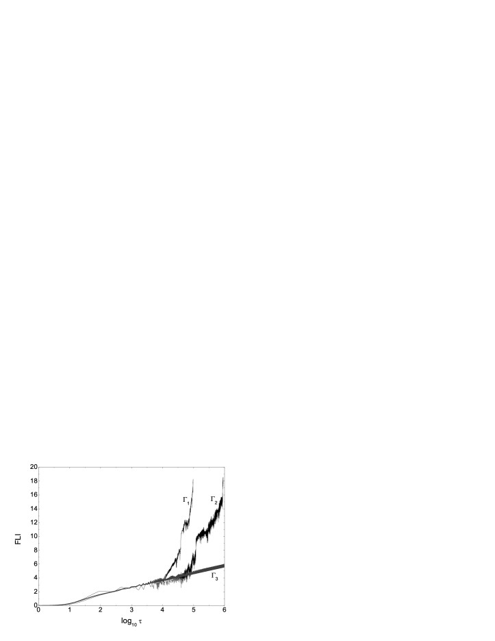
Figure 1: Same as Fig. 3 of Ref. [15], which describes the invariant FLI as a function of proper time for each of three orbits. Orbits $\Gamma_{1}$ and $\Gamma_{2}$ are chaotic, while orbit $\Gamma_{3}$ is not.

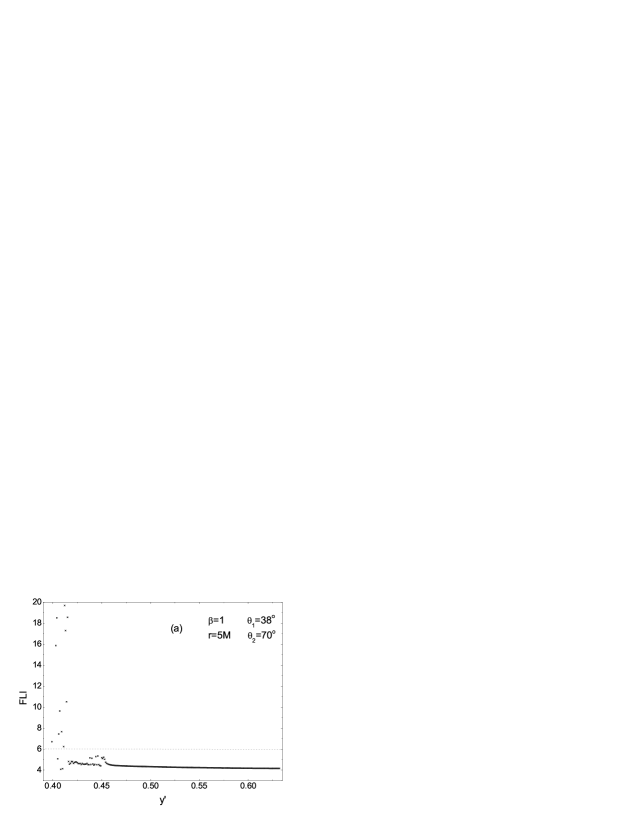
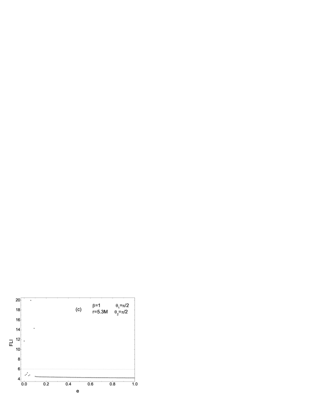
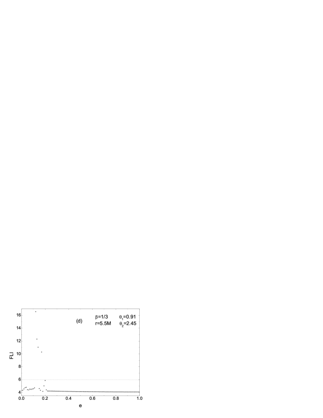
Figure 3: (a) FLI as a function of initial velocity $\dot{y}$. (b) same as (a) but for initial eccentricity $e$ in place of $\dot{y}$. (c) and (d) relate to the cases of distinct parameters and initial conditions adopted.

To illustrate the use of the invariant FLI, we begin by regenerating Fig. 3 of Ref. [15] in our Fig. 1, where the FLIs of three orbits vary with the proper time. Initial conditions and parameters of the three orbits are as follows. $\Gamma_{1}$: $(\mbox{\boldmath$x$},\mbox{\boldmath$v$})=(5.5M,0,0,0,0.4,0)$, $\beta=1/3$, $\chi_{\imath}=1~{}(\imath=1,2)$, and spin angles $\theta_{1}=\pi/2$ and $\theta_{2}=\pi/6$ so that initial spin configurations $\mbox{\boldmath$S$}_{\imath}=(S_{\imath}\sin\theta_{\imath},0,S_{\imath}\cos\theta_{\imath})$. $\Gamma_{2}$: $(\mbox{\boldmath$x$},\mbox{\boldmath$v$})=(5.0M,0,0,0,0.399,0)$, $\beta=1$, $\chi_{\imath}=1$, $\theta_{1}=38^{\circ}$, and $\theta_{2}=70^{\circ}$. $\Gamma_{3}$ is the same as $\Gamma_{2}$ but only 0.399 gives place to 0.428. In practice, the initial radius $r$ is equal to the first component $x$ of the initial relative coordinates for each case. In order to get their corresponding neighboring orbits, we add a very small deviation, $\Delta x=10^{-9}M$, to the $x$ only. As shown in Fig. 1, $\Gamma_{1}$ and $\Gamma_{2}$ are chaotic, but $\Gamma_{3}$ becomes ordered. The results are consistent with those of [7]. Obviously, chaos of $\Gamma_{1}$ gets rather stronger than that of $\Gamma_{2}$. In particular, the three orbits can be distinguished clearly as proper time arrives at $10^{5}M$.

Hereafter, each orbit does not stop computing till $\tau=10^{5}M$. It is shown with many numerical experiments that $FLI=6$ is a threshold between ordered and chaotic at this time. In detail, all orbits with $FLIs>6$ show chaos, while ones with $FLIs\leq 6$ signal regular. A point to note is that we shall hardly consider coalescing orbits during this time, but shall pay attention to stable orbits. Of course, increasing the integration time would reduce the number of the stable orbits. Since the invariant FLI has explicit merits, we shall borrow it to further gain an insight into the dynamics of spinning compact binaries.

III.1 Varying initial radii

Let us trace a dynamical sensitivity to the variations of some initial variables of the compact objects by taking $\Gamma_{1}$, $\Gamma_{2}$ and $\Gamma_{3}$ as basic references.

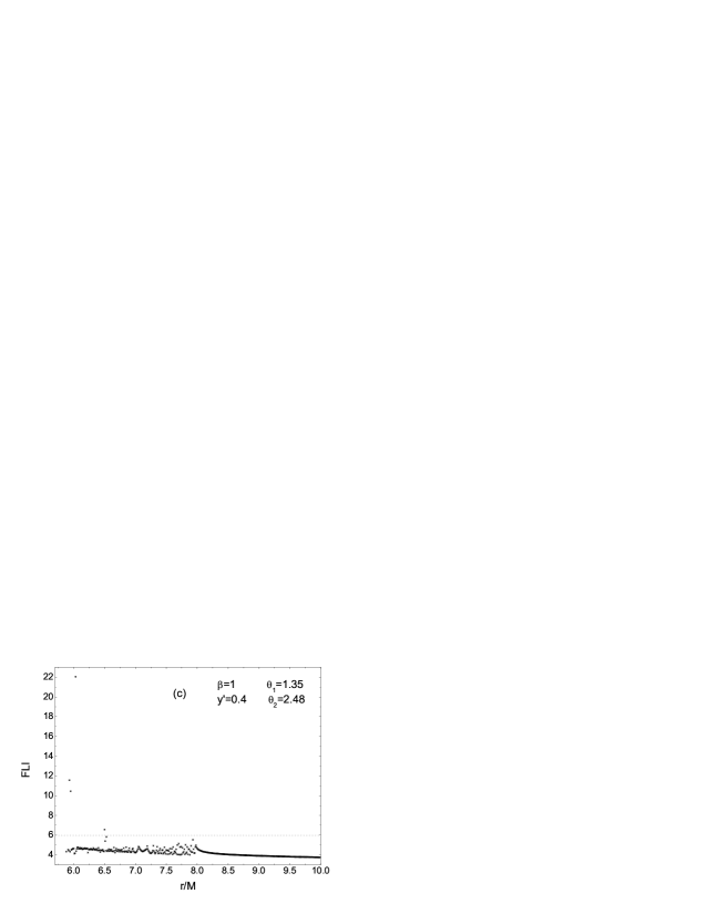
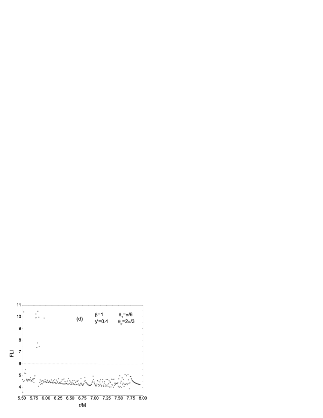
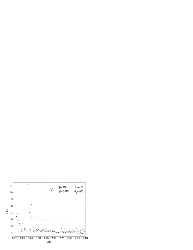
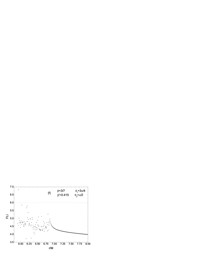
Figure 2: FLI as a function of initial radius $r$ for various parameters and other initial conditions.

Let us create a family of orbits with the same parameters and initial conditions as those of $\Gamma_{1}$ but the initial radius $r$ altered from $5.4M$ to $6M$. In terms of different values of FLIs, Fig. 2a describes that chaotic orbits are clustered at small radius regions of $r$ lower than $5.58M$. When different initial conditions and parameters $\dot{y}$, $\theta_{1}$, $\theta_{2}$ and $\beta$ are used, one can see the same fact from Figs. 2b-2f. There are two main reasons for leading to the result. A smaller possible radial separation corresponds to greater contributions to the PN terms in the equations of motion so that the nonlinear effects become stronger. On the other hand, it gives rise to the stronger spin coupling, as hinted in Eq. (3).

For an illustration, the presence of chaos at low radius regions was already mentioned by Hartl & Buonanno [9], who used another approximation, the PN ADM-Hamiltonian formulation for the same problem.

III.2 Varying initial eccentricities

Now, we observe the dynamical evolution with second initial component $\dot{y}$ of the relative velocity vector $v$ running from the interval [0.39, 0.633] according to Fig. 3a, where a number of orbits are consistent with $\Gamma_{2}$ in the parameters and the initial conditions except the $\dot{y}$. Without question, $\Gamma_{2}$ and $\Gamma_{3}$ are still two of all the orbits tested. Similar to Fig. 2, Fig. 3a displays that the onset of chaos is also at lower velocities less than about 0.42. In practice, the variation of $\dot{y}$ at the starting time corresponds to that of initial eccentricity when all the parameters and the other initial conditions are fixed. $\dot{y}=0.44721$ means the initial eccentricity $e=0$, which just corresponds to a quasicircular orbit of Newtonian two-body problems. Of course, the chaoticity of quasicircular orbits in relativistic two-body problems is possible for particular parameters and initial conditions (see Ref. [9]). In addition, $e$ becomes small with the growth of $\dot{y}$ when $\dot{y}<0.44721$ or large with the increase of $\dot{y}$ when $\dot{y}>0.44721$. In particular, we have $e=1$ for $\dot{y}=0.63245$. In addition, $e=0.2$ for $\Gamma_{2}$, while $e=0.08408$ for $\Gamma_{3}$. For details, see Fig. 3b, which plots $FLI$ vs initial eccentricity $e$ rather than $FLI$ vs $\dot{y}$ in Fig. 3a. Clearly, chaotic orbits are mainly concentrated on $e\approx 0.2$. However, Fig. 3c shows that chaos does occur near $e=0$ when we change the initial radius and spin angles, i.e. $r=5.3M$, $\theta_{1}=\theta_{2}=\pi/2$. On the other hand, it can still be seen from Fig. 3d that chaotic orbits are approximately located in $e=0.2$ when $r=5.5M$, $\beta=1/3$, $\theta_{1}=0.91$ and $\theta_{2}=2.45$. Of course, the relation for chaos dependence of initial eccentricity should vary if the parameters and the other initial conditions are different.

Meanwhile, Fig. 3 seems to tell us that any highly initial eccentricity does not bring chaos. Here we provide some details of the choice of the initial velocity $\dot{y}$ for a given initial eccentricity. In our various cases tested, we get $\dot{y}=\sqrt{(1+e)/r}$ or $\dot{y}=\sqrt{(1-e)/r}$ from the equation of $e=|r\dot{y}^{2}-1|$. In general, black hole binaries do not coalesce fast for highly initial eccentricity with larger starting velocity of $\dot{y}=\sqrt{(1+e)/r}$. In fact, all ordered orbits with high eccentricities in Fig. 3 are just corresponded to this case. On the contrary, for highly initial eccentricity with smaller starting velocity of $\dot{y}=\sqrt{(1-e)/r}$, the merger of black hole binaries appears so quicker that we have no way to detect chaos from order. In this sense, we cannot say that highly initial eccentricity with smaller starting velocity does not cause chaos. It has been reported that highly eccentric chaotic orbits with some particular parameters and initial conditions do exist in the corresponding ADM-Hamiltonian formulation [9].

The above facts show that eccentricity alone is not responsible for causing chaos. The result is the same as that of [8].

III.3 Varying binary mass ratio

Levin [8] investigated the binary mass ratio $\beta$ how to affect the bulk shape of the precession and gravitational wave modulation. As a result, the smaller the mass ratio is, the more prominent the effect of the precession becomes. Still, it has been unclear how much the mass ratio impacts the appearance of chaos. This is what we want to explore.

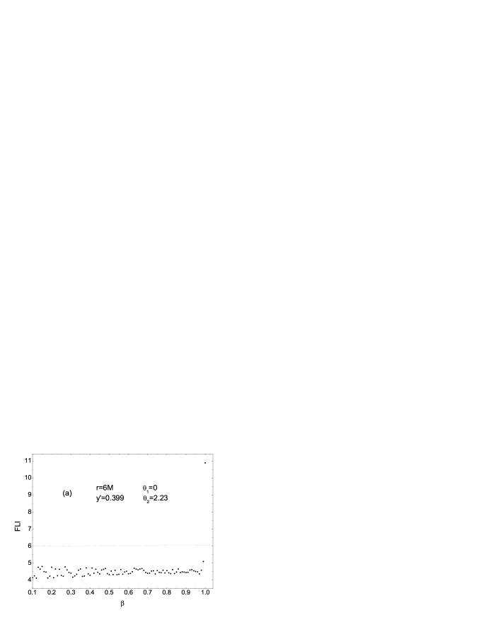
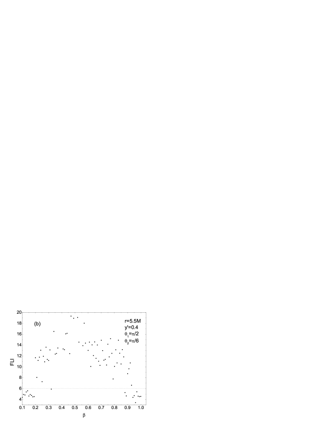
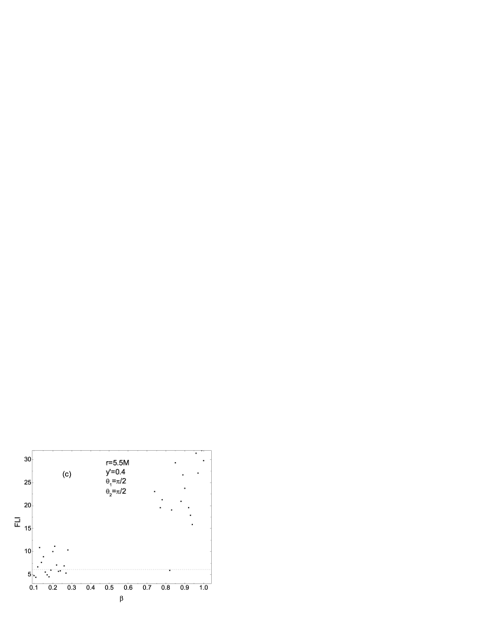
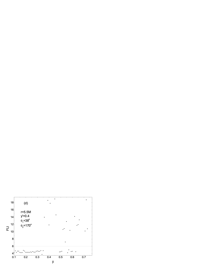
Figure 4: FLI as a function of binary mass ratio $\beta$. Specifically for panel (c), the blank interval with the binary mass ratios in the range of $\sim(0.3-0.7)$ represents the unstable coalescing orbits within the time considered. Some details of the FLI about the unstable orbits are neglected.

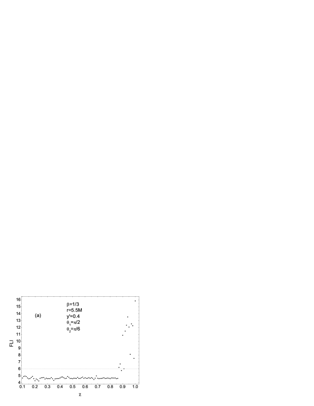
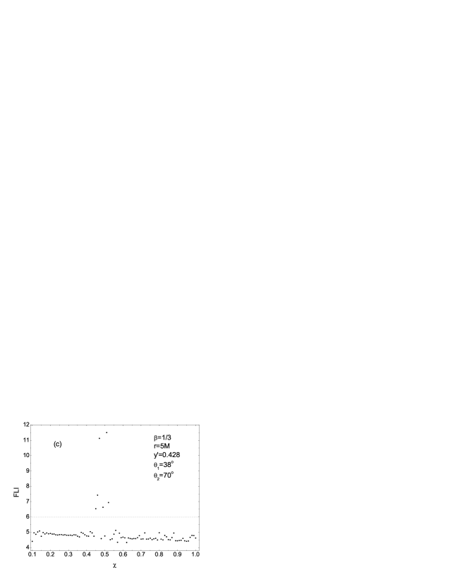
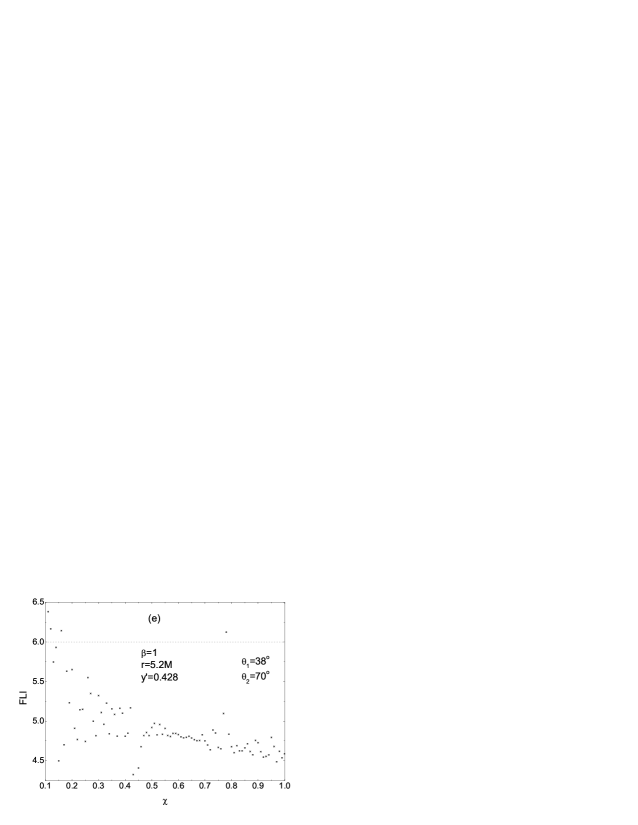
Figure 5: FLI as a function of dimensionless spin parameters $\chi=\chi_{1}=\chi_{2}$.

Hereafter we specify all orbits with initial conditions and parameters: $x=r$, $y=z=\dot{x}=\dot{z}=0$, $\chi_{1}=\chi_{2}=1$ (except Fig. 5), and with the others marked in each panel. As shown in Fig. 4a with $r=6M$, $\dot{y}=0.399$, $\theta_{1}=0$ and $\theta_{2}=2.23~{}radians$, the dynamics is typically ordered for huge numbers of values of $\beta$. A little attention to deserve is that a transition to chaos happens only when $\beta\approx 1$. However, the case is entirely different when we adopt $r=5.5M$, $\dot{y}=0.4$, $\theta_{1}=\pi/2$ and $\theta_{2}=\pi/6$ in Fig. 4b, which displays that chaos exists for most values of $\beta$. It is emphasized that chaos occurs neither for the maximum mass ratio nor for the minimum mass ratio. On the other hand, there are differently dynamical transitions with variations of $\beta$ if $r$, $\dot{y}$, $\theta_{1}$ and $\theta_{2}$ are changed into other fixed values like those given by Fig. 4c and 4d.

Therefore, it can be concluded from Fig. 4 that the mass ratio, $\beta$, can not be used only as a criterion for causing chaos or order. The larger or the smaller the mass ratio is, the stronger chaos does not necessarily get. There are various cases about the transitivity to chaos with the binary mass ratio varying for different combinations of fixed initial conditions and other parameters. A tentative interpretation to this thing is because the system studied has such many degrees of freedom and parameters that the dynamical features depend on not only $\beta$ but also the others. Once $\beta$ is varied (but the others are fixed and permitted to be chosen as variously possible values), it is not surprise to see the differently dynamical behaviors above.

III.4 Varying spin magnitudes

Levin [8] as well as Hartl & Buonanno [9] studied the effect of spinning up the lighter companion with some orbits. They pointed out that the larger the magnitude of the second spin becomes, the more irregular the motion is. Now let us use the invariant FLI to check this fact.

We take $\chi_{1}=\chi_{2}=\chi$, and then let $\chi$ range from 0.1 to 1. As expected, there is an abrupt transition to chaos in Fig. 5a when $\chi$ exceeds 0.86. It is worth emphasizing that chaos is incurred dramatically as $\chi$ increases. Only when $\theta_{2}=\pi/6$ in Fig. 5a gives place to $\theta_{2}=\pi/2$, are chaotic orbits in Fig. 5b mainly focused on the range of $\chi$ near 0.45. Still, there remains a rather small chaotic belt close to the maximal spins. If we set $r=5M$, $\dot{y}=0.428$, $\theta_{1}=38^{\circ}$ and $\theta_{2}=70^{\circ}$, chaos occurs when $\chi$ is nearly located in the middle of the interval. More details can be seen in Fig. 5c. On the other hand, chaos is completely absent for any spin magnitudes when we employ $r=5.2M$ instead of $r=5M$, as shown in Fig. 5d. With different parameters and initial conditions adopted, the dependence of chaos on $\chi$ alters at once (see Fig. 5e and 5f).

In our opinion, the maximal spins are not necessary to bring the strongest chaos. As stated in the above subsection, the spin magnitudes, as one of various factors to affect chaos, are not very sufficient to determine what dynamical feature the system is. Note that the result in the present paper should not be in conflict with those in Refs. [2,8], where only some particular conditions and parameters are considered.

III.5 Varying initial spin directions

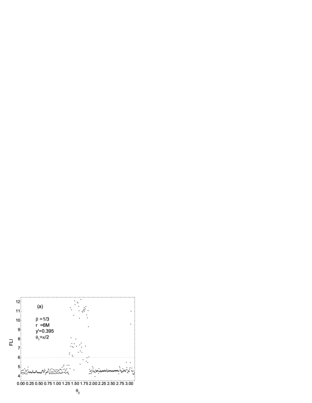
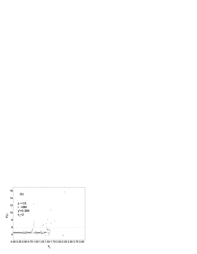
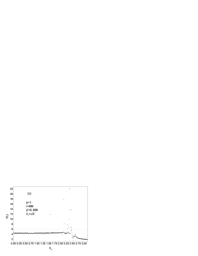
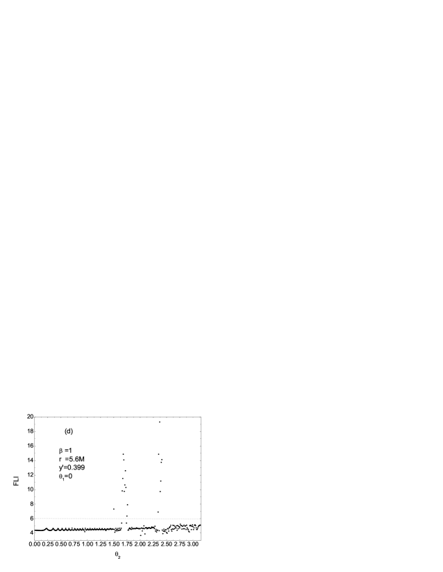
Figure 6: FLI as a function of initial spin alignment $\theta_{2}$.

In this subsection, we concentrate on demonstrating some dynamical sensitivity to the initial spin alignments. To do this, we fix the first initial spin angle $\theta_{1}$ of $\mbox{\boldmath$S$}_{1}$, and vary the second initial spin angle $\theta_{2}$ of $\mbox{\boldmath$S$}_{2}$ in $[0,\pi]$. Let us choose $\beta=1/3$, $r=6M$, $\dot{y}=0.395$ and $\theta_{1}=\pi/2$. It is shown with Fig. 6a that chaos is mainly trapped in the values of $\theta_{2}\approx\pi/2$. This seems to confirm the result of Refs. [2,8]. Of course, there is also a small chaotic region around $\theta_{2}\approx\pi$. If we change only the value of $\theta_{1}$ and obtain $\theta_{1}=2$, we find in Fig. 6b that there is a differently dynamical sensitivity to the initial spin angle $\theta_{2}$. In particular, the chaotic orbits are mainly clustered at values of $\theta_{2}$ around 2.25 rather than $\pi/2$ when we take $\beta=1$, $r=6M$, $\dot{y}=0.399$ and $\theta_{1}=\pi/2$ in Fig. 6c. The case is also different in Fig. 6d.

Clearly, the invariant FLI has been an invaluable and a computationally quicker tool to survey phase space for chaos by scanning huge numbers of orbits. Naturally, it is easy and suitable to study the dynamical structure of the $(\theta_{1},\theta_{2})$ plane. Let the two initial spin angles run from $[0,\pi]$ within a span of $\Delta\theta=0.01~{}radian$, respectively. At once, we have Figs. 7a-7d that give all the starting points in the plane according to distinct values of FLIs so that ordered and chaotic regions can be distinguished. In detail, the initial conditions in the $(\theta_{1},\theta_{2})$ plane are color coded black if $FLIs>6$ and gray when $FLIs\leq 6$. The black indicates chaos, but the gray means regular. By comparing between Figs. 7a and 7b or between Figs. 7c and 7d, we find again that the dynamical structures differ greatly for the different mass ratios. It should be pointed out that the structures in Fig. 7b/7d are symmetric since the pairs are of the same mass. As mentioned above, smaller initial radii lead still to the onset of stronger chaos. In addition, it can easily be seen that there is no chaos at all when the spins in each panel are nearly aligned with the orbital angular momentum, i.e. at the values near $\theta_{1}=\theta_{2}=0$. On the other hand, Eqs. (2) and (3) seem to show that the initial spins perpendicular to the orbital plane turn out to have the strong effects of the spin couplings. This seems to imply that the motion in the system becomes more irregular in this case. In fact, there is a stronger chaotic belt around $\theta_{1}=\theta_{2}=\pi/2$ of Fig. 7a. The result coincides basically with that of [8]. However, an important point to note is that the conservative system preserves only the spin magnitudes rather than the spin directions. Therefore, it should be reasonable that there are other chaotic regions far away values of $\theta_{1}=\theta_{2}=\pi/2$ in Fig. 7a when different combinations of other parameters and initial conditions are employed. Especially, it is no surprise that chaos disappears in a neighboring region of the point $(\pi/2,\pi/2)$ on the $(\theta_{1},\theta_{2})$ plane in Figs. 7c and 7d. As mentioned in the Introduction, Hartl & Buonanno [9] observed other cases from the PN Hamiltonian formulation, too.

In fact, each of Figs. 7a, 7b and 7d shows fractal boundaries at the basins of between stability (color-coded black and gray) and merger (color-coded white) in a slice through phase space. As Levin [2,8,12] pointed out, the fractal basin boundaries provide unambiguous signals of chaos. However, there is an exceptional case in which all the orbits of Fig. 7c are stable. This implies that the fractal basin boundary method is no longer fit for identifying the presence of chaos. Generally speaking, our method for establishing chaos hints the kernel of the fractal basin boundary method. Above all, the FLI is more universal in application, and gives more dynamical details than the fractal basin boundary method.

In the light of the above statements, we do not think that the initial spins perpendicular to the orbital plane can necessarily produce the strongest effect of chaos. There should be various ordered and chaotic regions on the $(\theta_{1},\theta_{2})$ plane if different combinations of other parameters and initial conditions are used. It should be worth noting that the results are not opposite to those in Refs. [2,8,9] with some particular parameters and initial conditions.

IV Conclusions

For conceptual clarity, it is physically significant to apply the invariant indicators of chaos, which are independent of the choice of spacetime coordinates, to study the orbital dynamics of relativistically gravitational systems. For spinning compact binaries, the coordinate time should be used in order to connect the relative motion of the bodies and their internal motions. In terms of this point and the 2PN metric of body 1 in the CM frame, it is able to construct the invariant indicators that measure the dynamical features of body 1, equivalently, ones of the relative motion. In this sense, it seems to be the most preferable to adopt the invariant Lyapunov exponent with two nearby trajectories [27]. Considering the too slow convergence of the Lyapunov exponent for the case of comparable mass binaries, we recommend the invariant FLI of two nearby trajectories in a curved spacetime [29], viewed as a very fast and valid technique to detect chaos from order.

A main contribution of the present paper is to discuss some applications of the invariant FLI in the study of dynamical transitions to chaos with the variations of parameters and initial conditions for the relativistic two-body system at 2PN order. Above all, this paper has been engaged to clarifying some doubt regarding the apparently conflicting results of chaos in the system from previous literatures. With this indicator we have successfully estimated effects of varying initial radii and velocities/eccentricities, varying binary mass ratios, varying spin magnitudes, and varying initial spin angles on the qualitative changes in the dynamical behaviors from nonchaotic to chaotic. For the specific choice of parameters and initial conditions, we recover some results of Levin [8] or Hartl & Buonanno [9], which include: (1) chaotic orbits are mainly clustered at initial low-radius regions; (2) eccentricity alone is not responsible for chaos; (3) the maximal spins increase the strength of chaos; (4) chaos becomes drastic when the initial spin vectors are nearly perpendicular to the orbital plane. However, when different combinations of the dynamical parameters and initial conditions are considered, a universal rule for the dependence of chaos on single parameter or initial condition cannot be found in general. That is to say, chaos does not depend only on the mass ratio. In addition, the maximal spins do not necessarily bring the strongest chaos. On the other hand, there are other large chaotic regions far away from the point $(\pi/2,\pi/2)$ in the $\theta_{1}$-$\theta_{2}$ plane. Even, chaos does disappear near the point $(\pi/2,\pi/2)$. A fundamental reason resulting from these facts is that a spinning compact binary system has so many degrees of freedom and parameters that only one physical parameter or initial condition is necessary but not sufficient to determine what dynamical behavior the system is. In short, no single physical parameter or initial condition can be described as responsible for causing chaos, but a complicated combination of all parameters and initial conditions.

It should be emphasized that the invariant FLI is a simple and firm tool to scan the global structure of phase space of the complicated spinning compact binary systems. Especially, the FLI is more universal to use, and gives more dynamical details than the fractal basin boundary method. As a result, the onset of the chaotic behavior for these systems at the 2PN expansion has been confirmed again.

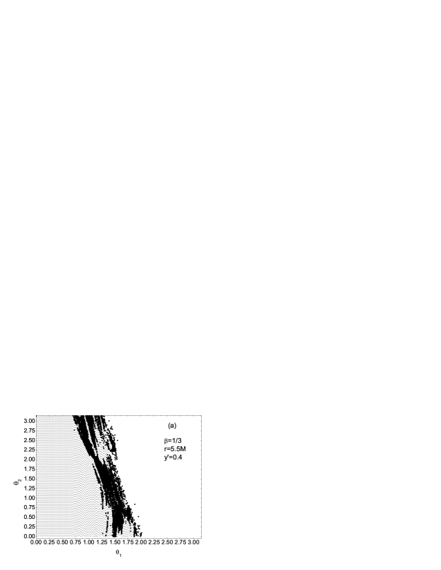
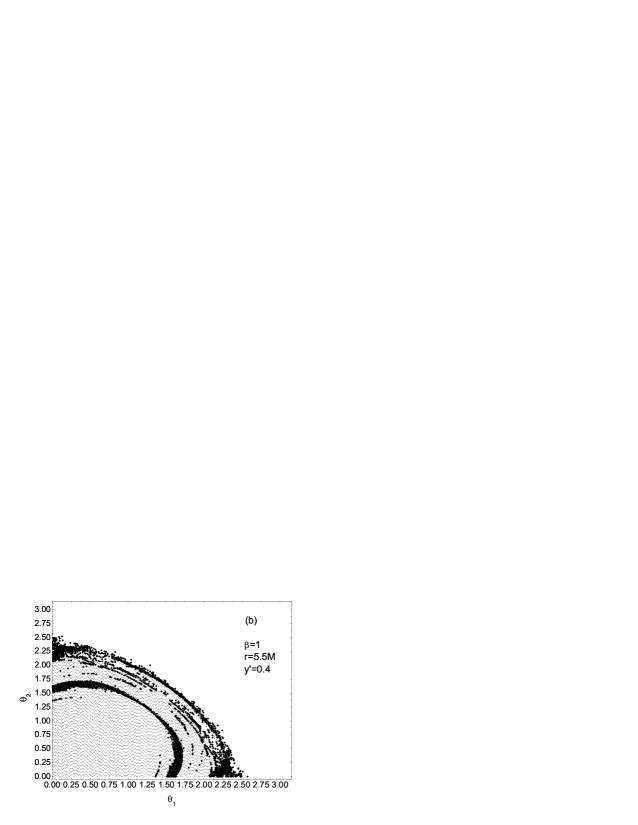
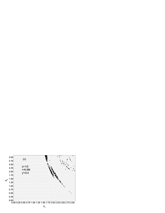
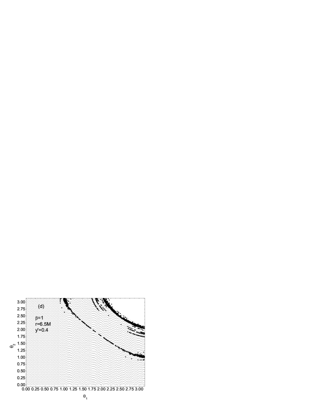
Figure 7: Scans of many groups of initial points in the $(\theta_{1},\theta_{2})$ plane. The black with $FLIs>6$ indicates chaos, but the gray with $FLIs\leq 6$ signals regular. As an illustration, $314\times 314$ orbits are computed in each of panels, and initial conditions color-coded white correspond to unstable merging pairs during the time scale integrated. Of course, the color-coded white regions should contain chaotic orbits as well as ordered ones. In particular, all the orbits in panel (c) are stable. This implies that the fractal basin boundary method becomes useless.

- (1) S. Suzuki and K. Maeda, Phys. Rev. D 55, 4848 (1997).
- (2) J. Levin, Phys. Rev. Lett. 84, 3515 (2000).
- (3) N.J. Cornish, Phys. Rev. Lett. 85, 3980 (2000).
- (4) N.J. Cornish, Phys. Rev. D 64, 084011 (2001).
- (5) J.D. Schnittman and F. A. Rasio, Phys. Rev. Lett. 87, 121101 (2001).
- (6) N.J. Cornish and J. Levin, Phys. Rev. Lett. 89, 179001 (2002).
- (7) N.J. Cornish and J. Levin, Phys. Rev. D 68, 024004 (2003).
- (8) J. Levin, Phys. Rev. D 67, 044013 (2003).
- (9) M.D. Hartl and A. Buonanno, Phys. Rev. D 71, 024027 (2005).
- (10) C. Königsdörffer and A. Gopakumar, Phys. Rev. D 71, 024039 (2005).
- (11) A. Gopakumar and C. Königsdörffer, Phys. Rev. D 72, 121501 (2005).
- (12) J. Levin, Phys. Rev. D 74, 124027 (2006).
- (13) Y. Xie and T.Y. Huang, Chinese J. Astron. Astrophys. 6, 705 (2006).
- (14) G. Tancredi, A. Sánchez, and F. Roig, Astron. J. 121, 1171 (2001).
- (15) X. Wu and Y. Xie, Phys. Rev. D 76, 124004 (2007).
- (16) C. Froeschlé and E. Lega, Celest. Mech. Dyn. Astron. 78, 167 (2000).
- (17) J. Laskar, Physica D 67, 257 (1993).
- (18) N. Voglis, G. Contopoulos, and C. Efthymiopoulos, Celest. Mech. Dyn. Astron. 73, 211 (1999).
- (19) Ch. Skokos, J. Phys. A 34, 10029 (2001).
- (20) G. Contopoulos, Order and Chaos in Dynamical Astronomy, Springer Verlag, (2002, 2004).
- (21) G. Contopoulos, N. Voglis and C. Efthymiopoulos, Celest. Mech. Dyn. Astron. 73, 1 (1999).
- (22) M. Szydlowski, Gen. Relativ. Gravit. 29, 185 (1997).
- (23) D. Hobill, D. Bernstein, D. Simpkmis and M. Welge, Classical Quantum Gravity 8, 1155 (1992).
- (24) G. Cushman and J. Sniatycki, Rep. Math. Phys. 36, 75 (1995).
- (25) G. Imponente and G. Montani, Phys. Rev. D 63, 103501 (2001).
- (26) A.E. Motter, Phys. Rev. Lett. 91, 231101 (2003).
- (27) X. Wu and T.Y. Huang, Phys. Lett. A 313, 77 (2003).
- (28) X. Wu and H. Zhang, Astrophys. J. 652, 1466 (2006).
- (29) X. Wu, T.Y. Huang and H. Zhang, Phys. Rev. D 74, 083001 (2006).
- (30) L. Blanchet, G. Faye and B. Ponsot, Phys. Rev. D 58, 124002 (1998).
- (31) H. Tagoshi, A. Ohashi and B.J. Owen, Phys. Rev. D 63, 044006 (2001).
- (32) L. Blanchet and B.R. Iyer, Classical Quantum Gravity 20, 755 (2003).
- (33) G. Faye, L. Blanchet and A. Buonanno, Phys. Rev. D 74, 104033 (2006).
- (34) L.E. Kidder, Phys. Rev. D 52, 821 (1995).
- (35) X. Wu, H. Zhang and X.S. Wan, Chinese J. Astron. Astrophys. 6, 125 (2006).
- (36) J.F. Zhu, X. Wu and D.Z. Ma, Chinese J. Astron. Astrophys. 7, 601 (2007).