Partial Dynamical Symmetries

Abstract

This overview focuses on the notion of partial dynamical symmetry (PDS), for which a prescribed symmetry is obeyed by a subset of solvable eigenstates, but is not shared by the Hamiltonian. General algorithms are presented to identify interactions, of a given order, with such intermediate-symmetry structure. Explicit bosonic and fermionic Hamiltonians with PDS are constructed in the framework of models based on spectrum generating algebras. PDSs of various types are shown to be relevant to nuclear spectroscopy, quantum phase transitions and systems with mixed chaotic and regular dynamics.

Keywords: Dynamical symmetry, partial symmetry, algebraic models, quantum phase transitions, regularity and chaos, pairing and seniority.

PACS numbers: 21.60.Fw, 03.65.Fd, 21.10.Re, 21.60.Cs, 05.45.-a

1 Introduction

Symmetries play an important role in dynamical systems. Constants of motion associated with a symmetry govern the integrability of a given classical system. At the quantum level, symmetries provide quantum numbers for the classification of states, determine spectral degeneracies and selection rules, and facilitate the calculation of matrix elements. An exact symmetry occurs when the Hamiltonian of the system commutes with all the generators ($g_{i}$) of the symmetry-group $G$, $[\,\hat{H}\,,\,g_{i}\,]=0$. In this case, all states have good symmetry and are labeled by the irreducible representations (irreps) of $G$. The Hamiltonian admits a block structure so that inequivalent irreps do not mix and all eigenstates in the same irrep are degenerate. In a dynamical symmetry the Hamiltonian commutes with the Casimir operator of $G$, $[\,\hat{H}\,,\,\hat{C}_{G}\,]=0$, the block structure of $\hat{H}$ is retained, the states preserve the good symmetry but, in general, are no longer degenerate. When the symmetry is completely broken then $[\,\hat{H}\,,\,g_{i}\,]\neq 0$, and none of the states have good symmetry. In-between these limiting cases there may exist intermediate symmetry structures, called partial (dynamical) symmetries, for which the symmetry is neither exact nor completely broken. This novel concept of symmetry and its implications for dynamical systems, in particular nuclei, are the focus of the present review.

Models based on spectrum generating algebras form a convenient framework to examine underlying symmetries in many-body systems and have been used extensively in diverse areas of physics [1]. Notable examples in nuclear physics are Wigner’s spin-isospin SU(4) supermultiplets [2], SU(2) single-$j$ pairing [3], Elliott’s SU(3) model [4], symplectic model [5], pseudo SU(3) model [6], Ginocchio’s monopole and quadrupole pairing models [7], interacting boson models (IBM) for even-even nuclei [8] and boson-fermion models (IBFM) for odd-mass nuclei [9]. Similar algebraic techniques have proven to be useful in the structure of molecules [10, 11] and of hadrons [12]. In such models the Hamiltonian is expanded in elements of a Lie algebra, ($G_{0}$), called the spectrum generating algebra. A dynamical symmetry occurs if the Hamiltonian can be written in terms of the Casimir operators of a chain of nested algebras, $G_{0}\supset G_{1}\supset\ldots\supset G_{n}$ [13]. The following properties are then observed. (i) All states are solvable and analytic expressions are available for energies and other observables. (ii) All states are classified by quantum numbers, $|\alpha_{0},\alpha_{1},\ldots,\alpha_{n}\rangle$, which are the labels of the irreps of the algebras in the chain. (iii) The structure of wave functions is completely dictated by symmetry and is independent of the Hamiltonian’s parameters.

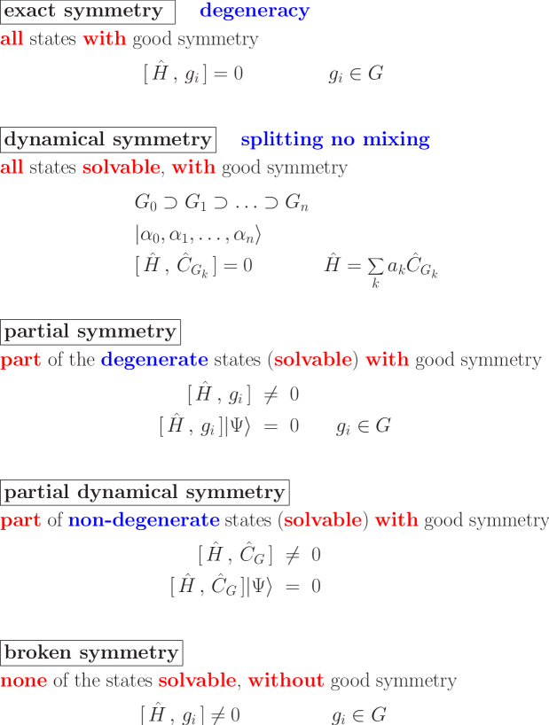
Figure 1: Hierarchy of symmetries.

A dynamical symmetry provides clarifying insights into complex dynamics and its merits are self-evident. However, in most applications to realistic systems, the predictions of an exact dynamical symmetry are rarely fulfilled and one is compelled to break it. The breaking of the symmetry is required for a number of reasons. First, one often finds that the assumed symmetry is not obeyed uniformly, i.e., is fulfilled by only some of the states but not by others. Certain degeneracies implied by the assumed symmetry are not always realized, (e.g., axially deformed nuclei rarely fulfill the IBM SU(3) requirement of degenerate $\beta$ and $\gamma$ bands [8]). Secondly, forcing the Hamiltonian to be invariant under a symmetry group may impose constraints which are too severe and incompatible with well-known features of nuclear dynamics (e.g., the models of [7] require degenerate single-nucleon energies). Thirdly, in describing transitional nuclei in-between two different structural phases, e.g., spherical and deformed, the Hamiltonian by necessity mixes terms with different symmetry character. In the models mentioned above, the required symmetry breaking is achieved by including in the Hamiltonian terms associated with (two or more) different sub-algebra chains of the parent spectrum generating algebra. In general, under such circumstances, solvability is lost, there are no remaining non-trivial conserved quantum numbers and all eigenstates are expected to be mixed. A partial dynamical symmetry (PDS) corresponds to a particular symmetry breaking for which some (but not all) of the virtues of a dynamical symmetry are retained. The essential idea is to relax the stringent conditions of complete solvability so that the properties (i)–(iii) are only partially satisfied. It is then possible to identify the following types of partial dynamical symmetries

• PDS type I:           part of the states have all the dynamical symmetry

• PDS type II:          all the states have part of the dynamical symmetry

• PDS type III:        part of the states have part of the dynamical symmetry.

In PDS of type I, only part of the eigenspectrum is analytically solvable and retains all the dynamical symmetry (DS) quantum numbers. In PDS of type II, the entire eigenspectrum retains some of the DS quantum numbers. PDS of type III has a hybrid character, in the sense that some (solvable) eigenstates keep some of the quantum numbers.

The notion of partial dynamical symmetry generalizes the concepts of exact and dynamical symmetries. In making the transition from an exact to a dynamical symmetry, states which are degenerate in the former scheme are split but not mixed in the latter, and the block structure of the Hamiltonian is retained. Proceeding further to partial symmetry, some blocks or selected states in a block remain pure, while other states mix and lose the symmetry character. A partial dynamical symmetry lifts the remaining degeneracies, but preserves the symmetry-purity of the selected states. The hierarchy of broken symmetries is depicted in Fig. 1.

The existence of Hamiltonians with partial symmetry or partial dynamical symmetry is by no means obvious. An Hamiltonian with the above property is not invariant under the group $G$ nor does it commute with the Casimir invariants of $G$, so that various irreps are in general mixed in its eigenstates. However, it posses a subset of solvable states, denoted by $|\Psi\rangle$ in Fig. 1, which respect the symmetry. The commutator $[\,\hat{H}\,,\,g_{i}\,]$ or $[\,\hat{H}\,,\,\hat{C}_{G}\,]$ vanishes only when it acts on these ‘special’ states with good $G$-symmetry.

In this review, we survey the various types of partial dynamical symmetries (PDS) and discuss algorithms for their realization in bosonic and fermionic systems. Hamiltonians with PDS are explicitly constructed, including higher-order terms. We present empirical examples of the PDS notion and demonstrate its relevance to nuclear spectroscopy, to quantum phase transitions and to mixed systems with coexisting regularity and chaos.

1.1 The interacting boson model

In order to illustrate the various notions of symmetries and consider their implications, it is beneficial to have a framework that has a rich algebraic structure and allows tractable yet detailed calculations of observables. Such a framework is provided by the interacting boson model (IBM) [8, 14, 15, 16], widely used in the description of low-lying quadrupole collective states in nuclei. The degrees of freedom of the model are one monopole boson ($s^{{\dagger}}$) and five quadrupole bosons ($d^{{\dagger}}_{\mu}$). The bilinear combinations $\{s^{{\dagger}}s,\,s^{{\dagger}}d_{\mu},\,d^{{\dagger}}_{\mu}s,\,d^{{\dagger}}_{\mu}d_{\mu^{\prime}}\}$ span a U(6) algebra. These generators can be transcribed in spherical tensor form as

$$\hat{n}_{s} = s^{{\dagger}}s\;\;,\;\;U^{(L)}_{\mu}=(d^{{\dagger}}\tilde{d})^{(L)}_{\mu}\quad L=0,1,2,3,4$$

$$\Pi^{(2)}_{\mu} = d^{{\dagger}}_{\mu}s+s^{{\dagger}}\tilde{d}_{\mu}\;\;,\;\;\bar{\Pi}^{(2)}_{\mu}=i(d^{{\dagger}}_{\mu}s-s^{{\dagger}}\tilde{d}_{\mu})~{},$$ (1)

where $\tilde{d}_{\mu}=(-1)^{\mu}d_{-\mu}$, and standard notation of angular momentum coupling is used. U(6) serves as the spectrum generating algebra and the invariant (symmetry) algebra is O(3), with generators $L^{(1)}_{\mu}=\sqrt{10}\,U^{(1)}_{\mu}$. The IBM Hamiltonian is expanded in terms of the operators (1) and consists of Hermitian, rotational-scalar interactions which conserve the total number of $s$- and $d$- bosons, $\hat{N}=\hat{n}_{s}+\hat{n}_{d}=s^{\dagger}s+\sum_{\mu}d^{\dagger}_{\mu}d_{\mu}$. Microscopic interpretation of the model suggests that for a given even-even nucleus the total number of bosons, $N$, is fixed and is taken as the sum of valence neutron and proton particle and hole pairs counted from the nearest closed shell [17].

The three dynamical symmetries of the IBM are

$$\begin{array}[]{lllllll}{\rm U(6)}&\supset&{\rm U(5)}&\supset{\rm O(5)}&\supset&{\rm O(3)}&\;{\rm anharmonic\;spherical\;vibrator}\\ {\rm U(6)}&\supset&{\rm SU(3)}&\supset{\rm O(3)}&&&\;{\rm axially}{\rm-deformed\;rotovibrator}\\ {\rm U(6)}&\supset&{\rm O(6)}&\supset{\rm O(5)}&\supset&{\rm O(3)}&\;\gamma{\rm-unstable\;deformed\;rotovibrator}\\ \end{array}$$ (5)

The associated analytic solutions resemble known limits of the geometric model of nuclei [18], as indicated above. Each chain provides a complete basis, classified by the irreps of the corresponding algebras, which can be used for a numerical diagonalization of the Hamiltonian in the general case. In the Appendix we collect the relevant information concerning the generators and Casimir operators of the algebras in Eq. (5). Electromagnetic moments and rates can be calculated in the IBM with transition operators of appropriate rank. For example, the most general one-body E2 operator reads

$$T(E2)=e_{B}\left[\,\Pi^{(2)}+\chi\,U^{(2)}\,\right]~{}.$$ (6)

A geometric visualization of the model is obtained by an energy surface

$$E_{N}(\beta,\gamma) = \langle\beta,\gamma;N|\hat{H}|\beta,\gamma;N\rangle~{},$$ (7)

defined by the expectation value of the Hamiltonian in the coherent (intrinsic) state [19, 20]

$$|\beta,\gamma;N\rangle = (N!)^{-1/2}(b^{\dagger}_{c})^{N}\,|0\,\rangle~{},$$ (8a)

$$b^{\dagger}_{c} = (1+\beta^{2})^{-1/2}[\beta\cos\gamma d^{\dagger}_{0}+\beta\sin{\gamma}(d^{\dagger}_{2}+d^{\dagger}_{-2})/\sqrt{2}+s^{\dagger}]~{}.$$ (8b)

Here $(\beta,\gamma)$ are quadrupole shape parameters whose values, $(\beta_{0},\gamma_{0})$, at the global minimum of $E_{N}(\beta,\gamma)$ define the equilibrium shape for a given Hamiltonian. The shape can be spherical $(\beta=0)$ or deformed $(\beta>0)$ with $\gamma=0$ (prolate), $\gamma=\pi/3$ (oblate), $\gamma$-independent, or triaxial $(0<\gamma<\pi/3)$. The latter shape requires terms of order higher than two-body in the boson Hamiltonian [21, 22]. The equilibrium deformations associated with the Casimir operators of the leading subalgebras in the dynamical symmetry chains (5) are, $\beta_{0}=0$ for U(5), $(\beta_{0}=\sqrt{2},\gamma_{0}=0)$ for SU(3) and $(\beta_{0}=1,\gamma_{0}\,{\rm arbitrary})$ for O(6).

2 PDS type I

PDS of type I corresponds to a situation for which the defining properties of a dynamical symmetry (DS), namely, solvability, good quantum numbers, and symmetry-dictated structure are fulfilled exactly, but by only a subset of states. An algorithm for constructing Hamiltonians with this property has been developed in [23] and further elaborated in [24]. The analysis starts from the chain of nested algebras

$$\begin{array}[]{ccccccc}G_{\rm dyn}&\supset&G&\supset&\cdots&\supset&G_{\rm sym}\\ \downarrow&&\downarrow&&&&\downarrow\\[0.0pt] [h]&&\langle\Sigma\rangle&&&&\Lambda\end{array}$$ (9)

where, below each algebra, its associated labels of irreps are given. Eq. (9) implies that $G_{\rm dyn}$ is the dynamical (spectrum generating) algebra of the system such that operators of all physical observables can be written in terms of its generators [11, 13]; a single irrep of $G_{\rm dyn}$ contains all states of relevance in the problem. In contrast, $G_{\rm sym}$ is the symmetry algebra and a single of its irreps contains states that are degenerate in energy. A frequently encountered example is $G_{\rm sym}={\rm O}(3)$, the algebra of rotations in 3 dimensions, with its associated quantum number of total angular momentum $L$. Other examples of conserved quantum numbers can be the total spin $S$ in atoms or total isospin $T$ in atomic nuclei.

The classification (9) is generally valid and does not require conservation of particle number. Although the extension from DS to PDS can be formulated under such general conditions, let us for simplicity assume in the following that particle number is conserved. All states, and hence the representation $[h]$, can then be assigned a definite particle number $N$. For $N$ identical particles the representation $[h]$ of the dynamical algebra $G_{\rm dyn}$ is either symmetric $[N]$ (bosons) or antisymmetric $[1^{N}]$ (fermions) and will be denoted, in both cases, as $[h_{N}]$. For particles that are non-identical under a given dynamical algebra $G_{\rm dyn}$, a larger algebra can be chosen such that they become identical under this larger algebra (generalized Pauli principle). The occurrence of a DS of the type (9) signifies that the Hamiltonian is written in terms of the Casimir operators of the algebras in the chain

$$\hat{H}_{DS} = \sum_{G}a_{G}\,\hat{C}_{G}$$ (10)

and its eigenstates can be labeled as $|[h_{N}]\langle\Sigma\rangle\dots\Lambda\rangle$; additional labels (indicated by $\dots$) are suppressed in the following. Likewise, operators can be classified according to their tensor character under (9) as $\hat{T}_{[h_{n}]\langle\sigma\rangle\lambda}$.

Of specific interest in the construction of a PDS associated with the reduction (9), are the $n$-particle annihilation operators $\hat{T}$ which satisfy the property

$$\hat{T}_{[h_{n}]\langle\sigma\rangle\lambda}|[h_{N}]\langle\Sigma_{0}\rangle\Lambda\rangle=0,$$ (11)

for all possible values of $\Lambda$ contained in a given irrep $\langle\Sigma_{0}\rangle$ of $G$. Any $n$-body, number-conserving normal-ordered interaction written in terms of these annihilation operators and their Hermitian conjugates (which transform as the corresponding conjugate irreps)

$$\hat{H}^{\prime} = \sum_{\alpha,\beta}A_{\alpha\beta}\,\hat{T}^{{\dagger}}_{\alpha}\hat{T}_{\beta}$$ (12)

has a partial G-symmetry. This comes about since for arbitrary coefficients, $A_{\alpha\beta}$, $\hat{H}^{\prime}$ is not a G-scalar, hence most of its eigenstates will be a mixture of irreps of G, yet relation (11) ensures that a subset of its eigenstates $|[h_{N}]\langle\Sigma_{0}\rangle\Lambda\rangle$, are solvable and have good quantum numbers under the chain (9). An Hamiltonian with partial dynamical symmetry is obtained by adding to $\hat{H}^{\prime}$ the dynamical symmetry Hamiltonian, $\hat{H}_{DS}$ (10), still preserving the solvability of states with $\langle\Sigma\rangle=\langle\Sigma_{0}\rangle$

$$\hat{H}_{PDS} = \hat{H}_{DS}+\hat{H}^{\prime}~{}.$$ (13)

If the operators $\hat{T}_{\beta}\equiv\hat{T}_{[h_{n}]\langle\sigma\rangle\lambda}$ span the entire irrep $\langle\sigma\rangle$ of G, then the annihilation condition (11) is satisfied for all $\Lambda$-states in $\langle\Sigma_{0}\rangle$, if none of the $G$ irreps $\langle\Sigma\rangle$ contained in the $G_{\rm dyn}$ irrep $[h_{N-n}]$ belongs to the $G$ Kronecker product $\langle\sigma\rangle\times\langle\Sigma_{0}\rangle$. So the problem of finding interactions that preserve solvability for part of the states (9) is reduced to carrying out a Kronecker product. In this case, although the generators $g_{i}$ of $G$ do not commute with $\hat{H}^{\prime}$, their commutator does vanish when it acts on the solvable states (11)

$$\left[\,g_{i}\,,\hat{H}^{\prime}\,\right] \neq 0~{},$$ (14a)

$$\left[\,g_{i}\,,\hat{H}^{\prime}\,\right]|[h_{N}]\langle\Sigma_{0}\rangle\Lambda\rangle = 0~{},\quad g_{i}\in G~{}.$$ (14b)

Eq. (14b) follows from $\left[\,g_{i}\,,\,\hat{T}^{{\dagger}}_{\alpha}\hat{T}_{\beta}\,\right]=\hat{T}^{{\dagger}}_{\alpha}\,\left[\,g_{i}\,,\hat{T}_{\beta}\,\right]+\left[\,g_{i}\,,\hat{T}^{{\dagger}}_{\alpha}\,\right]\hat{T}_{\beta}$ and the fact that $\left[\,g_{i}\,,\hat{T}_{\beta}\,\right]$ involves a linear combination of $G$-tensor operators which satisfy Eq. (11). The arguments for choosing the special irrep $\langle\Sigma\rangle=\langle\Sigma_{0}\rangle$ in Eq. (11), which contains the solvable states, are based on physical grounds. A frequently encountered choice is the irrep which contains the ground state of the system.

The above algorithm for constructing Hamiltonians with PDS of type I is applicable to any semisimple group. It can also address more general scenarios, in which relation (11) holds only for some states $\Lambda$ in the irrep $\langle\Sigma_{0}\rangle$ and/or some components $\lambda$ of the tensor $\hat{T}_{[h_{n}]\langle\sigma\rangle\lambda}$. In this case, the Kronecker product rule does not apply, yet the PDS Hamiltonian is still of the form as in Eqs. (12)-(13), but now the solvable states span only part of the corresponding $G$-irrep. This is not the case in the quasi-exactly solvable Hamiltonians, introduced in [25], where the solvable states form complete representations. The coexistence of solvable and unsolvable states, together with the availability of an algorithm, distinguish the notion of PDS from the notion of accidental degeneracy [26], where all levels are arranged in degenerate multiplets.

An Hamiltonian with PDS of type I does not have good symmetry but some of its eigenstates do. The symmetry of the latter states does not follow from invariance properties of the Hamiltonian. This situation is opposite to that encountered in a spontaneous symmetry breaking, where the Hamiltonian respects the symmetry but its ground state breaks it. The notion of PDS differs also from the notion of quasi-dynamical symmetry [27]. The latter corresponds to a situation in which selected states in a system continue to exhibit characteristic properties (e.g., energy and B(E2) ratios) of a dynamical symmetry, in the face of strong symmetry-breaking interactions. Such an “apparent” persistence of symmetry is due to the coherent nature of the mixing in the wave functions of these states. In contrast, in a PDS of type I, although the symmetry is broken (even strongly) in most states, the subset of solvable states preserve it exactly. In this sense, the symmetry is partial but exact!.

In what follows we present concrete constructions of Hamiltonians with PDS associated with the three DS chains (5) of the IBM. The partial symmetries in question involve continuous Lie groups. PDS can, however, be associated also with discrete groups which are relevant, e.g., to molecular physics. An example of a partial symmetry which involves point groups was presented in [28], employing a model of coupled anharmonic oscillators to describe the molecule $XY_{6}$. The partial symmetry of the Hamiltonian allowed a derivation of analytic expressions for the energies and eigenstates of a set of unique levels. Furthermore, the numerical calculations required to obtain the energies of the remaining (non-unique) levels were greatly simplified since the Hamiltonian could be diagonalized in a much smaller space.

2.1 U(5) PDS (type I)

The U(5) DS chain of the IBM and related quantum numbers are given by [14]

$$\begin{array}[]{ccccccc}{\rm U}(6)&\supset&{\rm U}(5)&\supset&{\rm O}(5)&\supset&{\rm O}(3)\\ \downarrow&&\downarrow&&\downarrow&&\downarrow\\[0.0pt] [N]&&\langle n_{d}\rangle&&(\tau)&n_{\Delta}&L\end{array}~{},$$ (18)

where the generators of the above groups are defined in Table 16 of the Appendix. For a given U(6) irrep $[N]$, the allowed U(5) and O(5) irreps are $n_{d}=0,1,2,\ldots,N$ and $\tau=n_{d},\,n_{d}-2,\dots 0$ or $1$, respectively. The values of $L$ contained in the O(5) irrep $(\tau)$, are obtained by partitioning $\tau=3n_{\Delta}~{}+~{}\lambda$, with $n_{\Delta},\,\lambda\geq 0$ integers, and $L=2\lambda,\,2\lambda-2,2\lambda-3,\ldots,\lambda$. The multiplicity label $n_{\Delta}$ in the ${\rm O(5)}\supset{\rm O(3)}$ reduction, counts the maximum number of $d$-boson triplets coupled to $L=0$ [29]. The eigenstates $|[N]\langle n_{d}\rangle(\tau)n_{\Delta}LM\rangle$ are obtained with a Hamiltonian with U(5) DS which, for one- and two-body interactions, can be transcribed in the form

$$\hat{H}_{\rm DS} = \epsilon\,\hat{n}_{d}+A\,\hat{n}_{d}(\hat{n}_{d}+4)+B\,\hat{C}_{{\rm O(5)}}+C\,\hat{C}_{{\rm O(3)}}~{}.$$ (19)

Here $\hat{n}_{d}$ and $\hat{n}_{d}(\hat{n}_{d}+4)$ are the linear and quadratic Casimir operators of U(5), respectively, and $\hat{C}_{G}$ denotes the quadratic Casimir operator of $G$, as defined in the Appendix. The Casimir operators of U(6) are omitted from Eq. (19) since they are functions of the total boson number operator, $\hat{N}=\hat{n}_{s}+\hat{n}_{d}$, which is a constant for all $N$-boson states. The spectrum of $\hat{H}_{\rm DS}$ is completely solvable with eigenenergies

$$E_{\rm DS} = \epsilon\,n_{d}+A\,n_{d}(n_{d}+4)+B\,\tau(\tau+3)+\,C\,L(L+1).$$ (20)

The U(5)-DS spectrum of Eq. (20) resembles that of an anharmonic spherical vibrator, describing quadrupole excitations of a spherical shape. The splitting of states in a given U(5) multiplet, $\langle n_{d}\rangle$, is governed by the O(5) and O(3) terms in $\hat{H}_{\rm DS}$ (19). The lowest U(5) multiplets involve states with quantum numbers $(n_{d}=0,\,\tau=0,\,L=0)$, $(n_{d}=1,\,\tau=1,\,L=2)$, and $(n_{d}=2,\,\tau=0,\,L=0)$, $(n_{d}=2,\,\tau=2,\,L=2,4)$.

Table 1: Normalized one- and two-boson U(5) tensors.

$n$	$n_{d}$	$\tau$	$n_{\Delta}$	$\ell$	$\hat{B}^{\dagger}_{[n]\langle n_{d}\rangle(\tau)n_{\Delta}\ell m}$
1	0	0	0	0	$s^{{\dagger}}$
1	1	1	0	2	$d^{{\dagger}}_{m}$
2	0	0	0	0	$\sqrt{\frac{1}{2}}(s^{{\dagger}})^{2}$
2	1	1	0	2	$s^{{\dagger}}d^{{\dagger}}_{m}$
2	2	0	0	0	$\sqrt{\frac{1}{2}}(d^{{\dagger}}d^{{\dagger}})^{(0)}_{0}$
2	2	2	0	2	$\sqrt{\frac{1}{2}}(d^{\dagger}d^{\dagger})^{(2)}_{m}$
2	2	2	0	4	$\sqrt{\frac{1}{2}}(d^{\dagger}d^{\dagger})^{(4)}_{m}$

The construction of Hamiltonians with U(5)-PDS is based on identification of $n$-boson operators which annihilate all states in a given U(5) irrep $\langle n_{d}\rangle$. A physically relevant choice is the irrep $n_{d}=0$ which consists of the ground state, with $\tau=L=0$, built of $N$ $s$-bosons

$$|[N],n_{d}=\tau=L=0\rangle = (N!)^{-1/2}\,(s^{{\dagger}})^{N}|0\rangle~{}.$$ (21)

Considering U(5) tensors, $\hat{B}^{\dagger}_{[n]\langle n_{d}\rangle(\tau)n_{\Delta}\ell m}$, composed of $n$ bosons of which $n_{d}$ are $d$-bosons then, clearly, the Hermitian conjugate of such operators with $n_{d}\neq 0$ will annihilate the $n_{d}=0$ state of Eq. (21). Explicit expressions for $n$-boson U(5) tensors, with $n=1,2$ are shown in Table 1. From them one can construct the following one- and two-body Hamiltonian with U(5)-PDS

$$\hat{H}_{PDS} = \epsilon_{d}\,d^{{\dagger}}\cdot\tilde{d}+u_{2}\,s^{{\dagger}}d^{{\dagger}}\cdot\tilde{d}s+v_{2}\,\left[\,s^{{\dagger}}d^{{\dagger}}\cdot(\tilde{d}\tilde{d})^{(2)}+H.c.\,\right]$$ (22)

$$+\sum_{L=0,2,4}c_{L}\,(d^{{\dagger}}d^{{\dagger}})^{(L)}\cdot(\tilde{d}\tilde{d})^{(L)}~{},$$

where $H.c.$ means Hermitian conjugate. By construction,

$$\hat{H}_{PDS}|[N],n_{d}=\tau=L=0\rangle = 0~{}.$$ (23)

Using Eq. (217), we can rewrite $\hat{H}_{PDS}$ in the form

$$\hat{H}_{PDS} = \hat{H}_{DS}+\hat{V}_{2}~{},$$ (24)

where $\hat{H}_{DS}$ is the U(5) dynamical symmetry Hamiltonian, Eq. (19), and $\hat{V}_{2}$ is given by

$$\hat{V}_{2} = v_{2}\left[\,s^{{\dagger}}d^{{\dagger}}\cdot(\tilde{d}\tilde{d})^{(2)}+H.c.\,\right]=v_{2}\,\Pi^{(2)}\cdot U^{(2)}=v_{2}\,U^{(2)}\cdot\Pi^{(2)}~{}.$$ (25)

The operators $\Pi^{(2)}_{\mu}$ and $U^{(2)}_{\mu}$ are defined in Eq. (1). The $\hat{V}_{2}$ term breaks the U(5) DS, however, it still has the U(5) basis states with $(n_{d}=\tau=L=0)$, Eq. (23), and $(n_{d}=\tau=L=3)$ as zero-energy eigenstates

$$\hat{V}_{2}\,|[N],n_{d}=\tau=L=3\rangle = 0~{}.$$ (26)

The last property follows from the U(5) selection rules of $\hat{V}_{2}$, $\Delta n_{d}=\pm 1$, and the fact that the irreps $(n_{d}=4,\tau=0,2,4)$ and $(n_{d}=2,\tau=0,2)$ do not contain an $L=3$ state. Altogether, $\hat{H}_{PDS}$ (24) is not diagonal in the U(5) chain, but retains the following solvable U(5) basis states with known eigenvalues

$$|[N],n_{d}=\tau=L=0\rangle\;\;\;\; E_{PDS}=0~{},$$ (27a)

$$|[N],n_{d}=\tau=L=3\rangle\;\;\;\; E_{PDS}=3\epsilon+21A+18B+12C~{}.\qquad\qquad$$ (27b)

As will be discussed in Section 6, this class of Hamiltonians with U(5)-PDS of type I is relevant to first-order quantum shape-phase transitions in nuclei.

A second class of Hamiltonians with U(5)-PDS can be obtained by considering the interaction

$$\hat{V}_{0} = v_{0}\left[\,(s^{{\dagger}})^{2}\tilde{d}\cdot\tilde{d}+H.c.\,\right]~{}.$$ (28)

This interaction breaks the U(5) DS, however, it still has selected U(5) basis states as zero-energy eigenstates

$$\hat{V}_{0}\,|[N],n_{d}=\tau=N,L\,\rangle = 0~{},$$ (29a)

$$\hat{V}_{0}\,|[N],n_{d}=\tau=N-1,L\,\rangle = 0~{},$$ (29b)

where $L$ takes the values compatible with the ${\rm O(5)}\supset{\rm O(3)}$ reduction. These properties follow from the fact that $s^{2}$ annihilates states with $n_{s}=0,\,1$ ($n_{d}=N,\,N-1$) and $\tilde{d}\cdot\tilde{d}$ annihilates states with $n_{d}=\tau$ [14]. Adding the interaction $\hat{V}_{0}$ to the U(5) dynamical symmetry Hamiltonian $\hat{H}_{DS}$ (19), we obtain the following Hamiltonian with U(5)-PDS

$$\hat{H}_{PDS}^{\prime} = \hat{H}_{DS}+\hat{V}_{0}~{}.$$ (30)

$\hat{H}_{PDS}^{\prime}$ is not diagonal in the U(5) chain, but retains the following solvable U(5) basis states with known eigenvalues

$$|[N],n_{d}=\tau=N,L\,\rangle\;\;\qquad\quad E_{PDS}^{\prime}=N[\,\epsilon_{d}+A(N+4)+B(N+3)\,]+CL(L+1)~{},\qquad\qquad$$ (31a)

$$|[N],n_{d}=\tau=N-1,L\,\rangle\;\;\;\quad E_{PDS}^{\prime}=(N-1)[\,\epsilon_{d}+A(N+3)+B(N+2)\,]+CL(L+1)~{}.\qquad\qquad$$ (31b)

The Hamiltonian $\hat{H}_{PDS}^{\prime}$ (30) with U(5)-PDS of type I, contains terms from both the U(5) and O(6) chains (5), hence preserves the common segment of subalgebras, ${\rm O(5)}\supset{\rm O(3)}$. As such, it exhibits also an O(5)-PDS of type II, to be discussed in Section 3. As will be shown in Section 6, this class of Hamiltonians is relevant to second-order quantum shape-phase transitions in nuclei.

2.2 SU(3) PDS (type I)

The SU(3) DS chain of the IBM and related quantum numbers are given by [15]

$$\begin{array}[]{ccccc}{\rm U}(6)&\supset&{\rm SU}(3)&\supset&{\rm O}(3)\\ \downarrow&&\downarrow&&\downarrow\\[0.0pt] [N]&&\left(\lambda,\mu\right)&K&L\end{array}~{},$$ (35)

where the generators of the above groups $G$ are defined in Table 16 of the Appendix. For a given U(6) irrep $[N]$, the allowed SU(3) irreps are $(\lambda,\mu)=(2N-4k-6m,2k)$ with $k,m$ non-negative integers, such that, $\lambda,\mu\geq 0$. The multiplicity label $K$ is needed for complete classification and corresponds geometrically to the projection of the angular momentum on the symmetry axis. The values of $L$ contained in the above SU(3) irreps are $L=K,K+1,K+2,\ldots,K+{\rm max}\{\lambda,\mu\}$, where $K=0,\,2,\ldots,{\rm min}\{\lambda,\mu\}$; with the exception of $K=0$ for which $L=0,\,2,\ldots,{\rm max}\{\lambda,\mu\}$. The states $|[N](\lambda,\mu)KLM\rangle$ form the (non-orthogonal) Elliott basis [4] and the Vergados basis $|[N](\lambda,\mu)\tilde{\chi}LM\rangle$ [30] is obtained from it by a standard orthogonalization procedure. The two bases coincide in the large-N limit and both are eigenstates of a Hamiltonian with SU(3) DS. The latter, for one- and two-body interactions, can be transcribed in the form

$$\hat{H}_{DS} = h_{2}\left[-\hat{C}_{{\rm SU(3)}}+2\hat{N}(2\hat{N}+3)\right]+C\,\hat{C}_{{\rm O(3)}}\quad~{},$$ (36)

where $\hat{C}_{G}$ is the quadratic Casimir operator of $G$, as defined in the Appendix. The spectrum of $\hat{H}_{DS}$ is completely solvable with eigenenergies

$$E_{\rm DS} = h_{2}\,\left[\,-f_{2}(\lambda,\mu)+2N(2N+3)\,\right]+C\,L(L+1)$$ (37)

$$= h_{2}\,6\left[2N(k+2m)-k(2k-1)-3m(2m-1)-6km\right]+CL(L+1)~{},\qquad$$

where $f_{2}(\lambda,\mu)=\lambda^{2}+\mu^{2}+\lambda\mu+3\lambda+3\mu$ and $(\lambda,\mu)=(2N-4k-6m,2k)$. The spectrum resembles that of an axially-deformed rotovibrator and the corresponding eigenstates are arranged in SU(3) multiplets. In a given SU(3) irrep $(\lambda,\mu)$, each $K$-value is associated with a rotational band and states with the same L, in different $K$-bands, are degenerate. The lowest SU(3) irrep is $(2N,0)$, which describes the ground band $g(K=0)$ of a prolate deformed nucleus. The first excited SU(3) irrep $(2N-4,2)$ contains both the $\beta(K=0)$ and $\gamma(K=2)$ bands. States in these bands with the same angular momentum are degenerate. This $\beta$-$\gamma$ degeneracy is a characteristic feature of the SU(3) limit of the IBM which, however, is not commonly observed [31]. In most deformed nuclei the $\beta$ band lies above the $\gamma$ band. In the IBM framework, with at most two-body interactions, one is therefore compelled to break SU(3) in order to conform with the experimental data. To do so, the usual approach has been to include in the Hamiltonian terms from other chains so as to lift the undesired $\beta$-$\gamma$ degeneracy. Such an approach was taken by Warner Casten and Davidson (WCD) in [32], where an O(6) term was added to the SU(3) Hamiltonian. However, in this procedure, the SU(3) symmetry is completely broken, all eigenstates are mixed and no analytic solutions are retained. Similar statements apply to the description in the consistent Q formalism (CQF) [33], where the Hamiltonian involves a non-SU(3) quadrupole operator. In contrast, partial SU(3) symmetry, to be discussed below, corresponds to breaking SU(3), but in a very particular way so that part of the states (but not all) will still be solvable with good symmetry. As such, the virtues of a dynamical symmetry (e.g., solvability) are fulfilled but by only a subset of states.

The construction of Hamiltonians with SU(3)-PDS is based on identification of $n$-boson operators which annihilate all states in a given SU(3) irrep $(\lambda,\mu)$, chosen here to be the ground band irrep $(2N,0)$. For that purpose, we consider the following boson-pair operators with angular momentum $L=0,\,2$

$$P^{\dagger}_{0} = d^{\dagger}\cdot d^{\dagger}-2(s^{\dagger})^{2}~{},$$ (38a)

$$P^{\dagger}_{2\mu} = 2d^{\dagger}_{\mu}s^{\dagger}+\sqrt{7}\,(d^{\dagger}\,d^{\dagger})^{(2)}_{\mu}~{}.$$ (38b)

Table 2: Normalized one- and two-boson SU(3) tensors. For the indicated irreps the labels of the Vergados basis ($\tilde{\chi}$) and Elliott basis ($K$) are identical, $\tilde{\chi}=K$.

$n$	$(\lambda,\mu)$	$\tilde{\chi}$	$\ell$	$\qquad\hat{B}^{\dagger}_{[n](\lambda,\mu)\tilde{\chi};\ell m}$
1	(2,0)	0	0	$s^{{\dagger}}$
1	(2,0)	0	2	$d^{{\dagger}}_{m}$
2	(4,0)	0	0	$\sqrt{\frac{5}{18}}(s^{{\dagger}})^{2}+\sqrt{\frac{2}{9}}(d^{{\dagger}}d^{{\dagger}})^{(0)}_{0}$
2	(4,0)	0	2	$\sqrt{\frac{7}{9}}s^{{\dagger}}d^{{\dagger}}_{m}-\frac{1}{3}(d^{{\dagger}}d^{{\dagger}})^{(2)}_{m}$
2	(4,0)	0	4	$\frac{1}{\sqrt{2}}(d^{{\dagger}}d^{{\dagger}})^{(4)}_{m}$
2	(0,2)	0	0	$-\sqrt{\frac{2}{9}}(s^{{\dagger}})^{2}+\sqrt{\frac{5}{18}}(d^{{\dagger}}d^{{\dagger}})^{(0)}_{0}\qquad$
2	(0,2)	0	2	$\sqrt{\frac{2}{9}}s^{{\dagger}}d^{{\dagger}}_{m}+\sqrt{\frac{7}{18}}(d^{{\dagger}}d^{{\dagger}})^{(2)}_{m}$

As seen from Table 2, these operators are proportional to two-boson SU(3) tensors, $B^{\dagger}_{[n](\lambda,\mu)\tilde{\chi};\ell m}$, with $n=2$ and $(\lambda,\mu)=(0,2)$

$$B^{\dagger}_{[2](0,2)0;00} = \frac{1}{3\sqrt{2}}\,P^{\dagger}_{0}~{},$$ (39a)

$$B^{\dagger}_{[2](0,2)0;2\mu} = \frac{1}{3\sqrt{2}}\,P^{\dagger}_{2\mu}~{}.$$ (39b)

The corresponding Hermitian conjugate boson-pair annihilation operators, $P_{0}$ and $P_{2\mu}$, transform as $(2,0)$ under SU(3), and satisfy

$$P_{0}\,|[N](2N,0)K=0,LM\rangle = 0~{},$$

$$P_{2\mu}\,|[N](2N,0)K=0,LM\rangle = 0~{}.$$ (40)

Equivalently, these operators satisfy

$$P_{0}|c;\,N\rangle = 0$$

$$P_{2\mu}|c;\,N\rangle = 0$$ (41)

where

$$|c;\,N\rangle = (N!)^{-1/2}(b^{{\dagger}}_{c})^{N}|0\rangle\;\;\;,\;\;\;b^{{\dagger}}_{c}=(\sqrt{2}\,d^{{\dagger}}_{0}+s^{{\dagger}})/\sqrt{3}~{}.$$ (42)

The state $|c;\,N\rangle$ is a condensate of $N$ bosons and is obtained by substituting the SU(3) equilibrium deformations in the coherent state of Eq. (8), $|c;\,N\rangle=|\beta=\sqrt{2},\gamma=0;N\rangle$. It is the lowest-weight state in the SU(3) irrep $(\lambda,\mu)=(2N,0)$ and serves as an intrinsic state for the SU(3) ground band [34]. The rotational members of the band $|[N](2N,0)K=0,LM\rangle$, Eq. (40), are obtained by angular momentum projection from $|c;\,N\rangle$. The relations in Eqs. (40)-(41) follow from the fact that the action of the operators $P_{L\mu}$ leads to a state with $N-2$ bosons in the U(6) irrep $[N-2]$, which does not contain the SU(3) irreps obtained from the product $(2,0)\times(2N,0)=(2N+2,0)\oplus(2N,1)\oplus(2N-2,2)$.

Following the general algorithm, a two-body Hamiltonian with partial SU(3) symmetry can now be constructed as [23, 35]

$$\hat{H}(h_{0},h_{2}) = h_{0}\,P^{\dagger}_{0}P_{0}+h_{2}\,P^{\dagger}_{2}\cdot\tilde{P}_{2}~{},$$ (43)

where $\tilde{P}_{2,\mu}=(-)^{\mu}P_{2,-\mu}$. For $h_{2}=h_{0}$, the Hamiltonian is an SU(3) scalar, related to the quadratic Casimir operator of SU(3)

$$\hat{H}(h_{0}=h_{2}) = h_{2}\,\left[P^{\dagger}_{0}P_{0}+P^{\dagger}_{2}\cdot\tilde{P}_{2}\right]=h_{2}\left[-\hat{C}_{{\rm SU(3)}}+2\hat{N}(2\hat{N}+3)\right]~{}.\qquad$$ (44)

For $h_{0}=-5h_{2}$, the Hamiltonian transforms as a $(2,2)$ SU(3) tensor component. For arbitrary $h_{0},h_{2}$ coefficients, $\hat{H}(h_{0},h_{2})$ is not an SU(3) scalar, nevertheless, the relations in Eqs. (40)-(41) ensure that it has a solvable zero-energy band with good SU(3) quantum numbers $(\lambda,\mu)=(2N,0)$. When the coefficients $h_{0},\,h_{2}$ are positive, $\hat{H}(h_{0},h_{2})$ becomes positive definite by construction, and the solvable states form its SU(3) ground band.

$\hat{H}(h_{0},h_{2})$ of Eq. (43) has additional solvable eigenstates with good SU(3) character. This comes about from Eq. (41) and the following properties

$$P_{L,\mu}|c;N\rangle\;=\;0\;\;\;,\;\;\;\left[P_{L,\mu}\,,\,P^{\dagger}_{2,2}\right]|c;N\rangle\;=\;\delta_{L,2}\delta_{\mu,2}\,6(2N+3)|c;N\rangle\;\;\;,\qquad$$

$$\left[\left[P_{L,\mu}\,,\,P^{\dagger}_{2,2}\right]\,,\,P^{\dagger}_{2,2}\right]\;=\;\delta_{L,2}\delta_{\mu,2}\,24P^{\dagger}_{2,2}\;\;\;,\qquad\quad L=0,2\quad~{}.$$ (45)

These relations imply that the sequence of states

$$|k\rangle\;\propto\;\left(P^{\dagger}_{2,2}\right)^{k}|c;N-2k\rangle~{},$$ (46)

are eigenstates of $\hat{H}(h_{0},h_{2})$ with eigenvalues $E_{k}\;=\;6h_{2}\left(2N+1-2k\right)k$. A comparison with Eq. (37) shows that these energies are the SU(3) eigenvalues of $\hat{H}(h_{0}=h_{2})$, Eq. (44), and identify the states $|k\rangle$ to be in the SU(3) irreps $(2N-4k,2k)$. They can be further shown to be the lowest-weight states in these irreps. Furthermore, $P_{0}$ satisfies

$$P_{0}\,|k\rangle = 0~{},$$ (47)

or equivalently,

$$P_{0}\,|[N](2N-4k,2k)K=2k,LM\rangle = 0~{}.$$ (48)

The states $|k\rangle$ (46) are deformed and serve as intrinsic states representing $\gamma^{k}$ bands with angular momentum projection ($K=2k$) along the symmetry axis [34]. In particular, as noted earlier, $|k=0\rangle=|c;N\rangle$ represents the ground band ($K=0$) and $|k=1\rangle$ is the $\gamma$-band ($K=2$). The rotational members of these bands, $|[N](2N-4k,2k)K=2k,LM\rangle\propto\hat{\cal P}_{LM}|k\rangle$, Eq. (48), can be obtained by O(3) projection from the corresponding intrinsic states $|k\rangle$. Relations (47) and (48) are equivalent, since the angular momentum projection operator, $\hat{\cal P}_{LM}$, is composed of O(3) generators, hence commutes with $P_{0}$. The intrinsic states $|k\rangle$ break the O(3) symmetry, but since the Hamiltonian in Eq. (43) is O(3) invariant, the projected states with good $L$ are also eigenstates of $\hat{H}(h_{0},h_{2})$ with energy $E_{k}$ and with good SU(3) symmetry. For the ground band $(k=0)$ the projected states span the entire SU(3) irrep $(2N,0)$. For excited bands $(k\neq 0)$, the projected states span only part of the corresponding SU(3) irreps. There are other states originally in these irreps (as well as in other irreps) which do not preserve the SU(3) symmetry and therefore get mixed. In particular, the ground $g(K=0)$, and $\gamma(K=2)$ bands retain their SU(3) character $(2N,0)$ and $(2N-4,2)$ respectively, but the first excited $K=0$ band is mixed. This situation corresponds precisely to that of partial SU(3) symmetry. An Hamiltonian $\hat{H}(h_{0},h_{2})$ which is not an SU(3) scalar has a subset of solvable eigenstates which continue to have good SU(3) symmetry.

All of the above discussion is applicable also to the case when we add to the Hamiltonian of Eq. (43) the Casimir operator of O(3), and by doing so, convert the partial SU(3) symmetry into partial dynamical SU(3) symmetry. The additional rotational term contributes just an $L(L+1)$ splitting but does not affect the wave functions. The most general one- and two-body Hamiltonian with SU(3)-PDS can thus be written in the form

$$\hat{H}_{PDS} = \hat{H}(h_{0},h_{2})+C\,\hat{C}_{{\rm O(3)}}=\hat{H}_{DS}+(h_{0}-h_{2})\,P^{\dagger}_{0}P_{0}~{}.$$ (49)

Here $\hat{H}_{DS}$ is the SU(3) dynamical symmetry Hamiltonian, Eq. (36), with parameters $h_{2}$ and $C$. The $P^{{\dagger}}_{0}P_{0}$ term in Eq. (49) is not diagonal in the SU(3) chain (35), but Eqs. (40) and (48) ensure that it annihilates a subset of states with good SU(3) quantum numbers. Consequently, $\hat{H}_{PDS}$ retains selected solvable bands with good SU(3) symmetry. Specifically, the solvable states are members of the ground $g(K=0)$ band

$$|N,(2N,0)K=0,L\rangle\;\;\;\;L=0,2,4,\ldots,2N$$ (50a)

$$E_{PDS}=CL(L+1)$$ (50b)

and $\gamma^{k}(K=2k)$ bands

$$|N,(2N-4k,2k)K=2k,L\rangle\;\;\;\;\;\;L=K,K+1,\ldots,(2N-2k)\qquad\qquad$$ (51a)

$$E_{PDS}=h_{2}\,6k\left(2N-2k+1\right)+CL(L+1)\qquad k>0~{}.$$ (51b)

The solvable states (50)-(51) are those projected from the intrinsic states $|k\rangle$ of Eq. (46), and are simply selected members of the Elliott basis $\phi_{E}((\lambda,\mu)KLM)$ [4]. In particular, the states belonging to the ground and $\gamma$ bands are the Elliott states $\phi_{E}((2N,0)K=0,LM)$ and $\phi_{E}((2N-4,2)K=2,LM)$ respectively. Their wave functions can be expressed in terms of the orthonormal Vergados basis, $\Psi_{V}((\lambda,\mu)\tilde{\chi}LM)$ [30]. For the ground band and for members of the $\gamma$ band with $L$ odd, the Vergados and Elliott bases are identical. The Elliott states in the $\gamma(K=2)$ band with $L$ even are mixtures of Vergados states in the SU(3) irrep $(2N-4,2)$

$$\phi_{E}((2N-4,2)K=2,LM)=$$

$$\qquad\quad\left[\,\Psi_{V}((2N-4,2)\tilde{\chi}=2,LM)-x^{(L)}_{20}\,\Psi_{V}((2N-4,2)\tilde{\chi}=0,LM)\,\right]/x^{(L)}_{22}~{},\qquad\quad$$ (52)

where $x^{(L)}_{20},\,x^{(L)}_{22}$ are known coefficients which appear in the transformation between the two bases [30].

Since the wave functions of the solvable states are known, it is possible to obtain analytic expressions for matrix elements of observables between them. For calculating E2 rates, it is convenient to rewrite the relevant E2 operator, Eq. (6), in the form

$$T(E2)\;=\;\alpha\,Q^{(2)}+\theta\,\Pi^{(2)}~{},$$ (53)

where $Q^{(2)}$ is the quadrupole SU(3) generator [$\,Q^{(2)}=\Pi^{(2)}-(\sqrt{7}/2)\,U^{(2)}\,$] and $\Pi^{(2)}$ is a $(2,2)$ tensor under SU(3). The B(E2) values for $g\to g$ and $g\to\gamma$ transitions

$$B(E2;g,L\rightarrow g,L^{\prime})=\qquad\qquad\qquad\qquad\qquad\qquad\qquad\qquad\qquad\qquad\qquad$$

$$\frac{|\langle\phi_{E}((2N,0)K=0,L^{\prime})||\alpha\,Q^{(2)}+\theta\,\Pi^{(2)}||\phi_{E}((2N,0)K=0,L)\rangle|^{2}}{(2L+1)}~{},$$ (54a)

$$B(E2;\gamma,L\rightarrow g,L^{\prime})=\qquad\qquad\qquad\qquad\qquad\qquad\qquad\qquad\qquad\qquad\qquad$$

$$\theta^{2}\,\frac{|\langle\phi_{E}((2N,0)K=0,L^{\prime})||\Pi^{(2)}||\phi_{E}((2N-4,2)K=2,L)\rangle|^{2}}{(2L+1)}~{}.$$ (54b)

can be expressed in terms of E2 matrix elements in the Vergados basis, for which analytic expressions are available [15, 36].

The Hamiltonian of Eq. (49), with SU(3)-PDS, was used in [35] to describe spectroscopic data of ¹⁶⁸Er. The experimental spectra [32] of the ground $g(K=0^{+}_{1})$, $\gamma(K=2^{+}_{1})$ and $K=0^{+}_{2}$ bands in this nucleus is shown in Fig. 2, and compared with an exact DS, PDS and broken SU(3) calculations.

Figure 2: Spectra of ¹⁶⁸Er ($N=16$). Experimental energies (EXP) are compared with IBM calculations in an exact SU(3) dynamical symmetry [SU(3)], in a broken SU(3) symmetry (WCD) [32] and in a partial dynamical SU(3) symmetry (PDS). The latter employs the Hamiltonian of Eq. (49) with $h_{0}=8,\,h_{2}=4,\,C=13$ keV. Adapted from [35].

Figure 3: SU(3) decomposition of wave functions of the ground ($K=0_{1}$), $\gamma$ ($K=2_{1}$), and $K=0_{2}$ bands of ¹⁶⁸Er ($N=16$) in a SU(3)-PDS calculation and in broken-SU(3) calculations: CQF [33] and WCD [32]. Adapted from [37].

According to the previous discussion, the SU(3)-PDS spectrum of the solvable ground and $\gamma$ bands is given by

$$E_{g}(L) = CL(L+1)~{},$$

$$E_{\gamma}(L) = 6h_{2}(2N-1)+CL(L+1)~{}.$$ (55)

$\hat{H}_{PDS}$ (49) is specified by three parameters (N=16 for ¹⁶⁸Er according to the usual boson counting). The values of $C$ and $h_{2}$ were extracted from the experimental energy differences $[E(2^{+}_{g})-E(0^{+}_{g})]$ and $[E(2^{+}_{\gamma})-E(2^{+}_{g})]$ respectively. The spectrum of an exact SU(3) DS, Eq. (37), obtained for $h_{0}=h_{2}$, deviates considerably from the experimental data since empirically the $K=0^{+}_{2}$ and $\gamma(K=2^{+}_{1})$ bands are not degenerate. In the SU(3)-PDS calculation, the parameter $h_{0}$ was varied so as to reproduce the bandhead energy of the $K=0^{+}_{2}$ band. The prediction for other rotational members of the $K=0^{+}_{1},\,0^{+}_{2},\,2^{+}_{1}$ bands is shown in Fig. 2. Clearly, the SU(3) PDS spectrum is an improvement over the schematic, exact SU(3) dynamical symmetry description, since the $\beta$-$\gamma$ degeneracy is lifted. The ground and $\gamma$ bands are solvable, still, the quality of the calculated PDS spectrum is similar to that obtained in the broken-SU(3) calculation (WCD) [32].

The resulting SU(3) decomposition of the lowest bands for the SU(3)-PDS calculation is shown in Fig. 3, and compared [37] to the conventional broken-SU(3) calculations WCD [32] and CQF [33]. In the latter calculations all states are mixed with respect to SU(3). In contrast, in the PDS calculation, the good SU(3) character, $(32,0)$ for the ground band and $(28,2)$ for $\gamma$ band, is retained, while the $K=0^{+}_{2}$ band contains about $13\%$ admixtures into the dominant $(28,2)$ irrep. Thus, the breaking of the SU(3) symmetry induced by $\hat{H}_{PDS}$ (49) is not small, and can lead to an appreciable SU(3) mixing in the remaining non-solvable states. Nevertheless, the special solvable states carry good SU(3) labels. The SU(3) symmetry is therefore partial but exact.

Table 3: B(E2) branching ratios from states in the $\gamma$ band in ¹⁶⁸Er. The column EXP lists the experimental ratios [32], PDS is the SU(3) partial dynamical symmetry calculation [35] and WCD is the broken SU(3) calculation [32]. Adapted from [35].

$L^{\pi}_{i}$	$L^{\pi}_{f}$	EXP	PDS	WCD		$L^{\pi}_{i}$	$L^{\pi}_{f}$	EXP	PDS	WCD
$2^{+}_{\gamma}$	$0^{+}_{g}$	$54.0$	$64.27$	$66.0$		$6^{+}_{\gamma}$	$4^{+}_{g}$	$0.44$	$0.89$	$0.97$
	$2^{+}_{g}$	$100.0$	$100.0$	$100.0$			$6^{+}_{g}$	$3.8$	$4.38$	$4.3$
	$4^{+}_{g}$	$6.8$	$6.26$	$6.0$			$8^{+}_{g}$	$1.4$	$0.79$	$0.73$
$3^{+}_{\gamma}$	$2^{+}_{g}$	$2.6$	$2.70$	$2.7$			$4^{+}_{\gamma}$	$100.0$	$100.0$	$100.0$
	$4^{+}_{g}$	$1.7$	$1.33$	$1.3$			$5^{+}_{\gamma}$	$69.0$	$58.61$	$59.0$
	$2^{+}_{\gamma}$	$100.0$	$100.0$	$100.0$		$7^{+}_{\gamma}$	$6^{+}_{g}$	$0.74$	$2.62$	$2.7$
$4^{+}_{\gamma}$	$2^{+}_{g}$	$1.6$	$2.39$	$2.5$			$5^{+}_{\gamma}$	$100.0$	$100.0$	$100.0$
	$4^{+}_{g}$	$8.1$	$8.52$	$8.3$			$6^{+}_{\gamma}$	$59.0$	$39.22$	$39.0$
	$6^{+}_{g}$	$1.1$	$1.07$	$1.0$		$8^{+}_{\gamma}$	$6^{+}_{g}$	$1.8$	$0.59$	$0.67$
	$2^{+}_{\gamma}$	$100.0$	$100.0$	$100.0$			$8^{+}_{g}$	$5.1$	$3.57$	$3.5$
$5^{+}_{\gamma}$	$4^{+}_{g}$	$2.91$	$4.15$	$4.3$			$6^{+}_{\gamma}$	$100.0$	$100.0$	$100.0$
	$6^{+}_{g}$	$3.6$	$3.31$	$3.1$			$7^{+}_{\gamma}$	$135.0$	$28.64$	$29.0$
	$3^{+}_{\gamma}$	$100.0$	$100.0$	$100.0$
	$4^{+}_{\gamma}$	$122.0$	$98.22$	$98.5$

Electromagnetic transitions are a more sensitive probe to the structure of states, hence are an important indicator for testing the predictions of SU(3)-PDS. Based on the analytic expressions of Eq. (54), the parameters $\alpha$ and $\theta$ of the E2 operator can be extracted from the experimental values of $B(E2;0^{+}_{g}\rightarrow 2^{+}_{g})$ and $B(E2;0^{+}_{g}\rightarrow 2^{+}_{\gamma})$. The corresponding ratio for ¹⁶⁸Er is $\theta/\alpha=4.261$. As shown in Table 3, the resulting SU(3) PDS E2 rates for transitions originating within the $\gamma$ band are found to be in excellent agreement with experiment and are similar to the WCD broken-SU(3) calculation [32]. In particular, the SU(3) PDS calculation reproduces correctly the $(\gamma\rightarrow\gamma)/(\gamma\rightarrow g)$ strengths. The only significant discrepancy is that for the $8^{+}_{\gamma}\rightarrow 7^{+}_{\gamma}$ transition which is very weak experimentally, with an intensity error of $50\%$ and an unknown M1 component [32]. The expressions in Eq. (54) imply that $\gamma\rightarrow g$ $B(E2)$ ratios are independent of both E2 parameters $\alpha$ and $\theta$. Furthermore, since the ground and $\gamma$ bands have pure SU(3) character, $(2N,0)$ and $(2N-4,2)$ respectively, the corresponding wave-functions do not depend on parameters of the Hamiltonian and hence are determined solely by symmetry. Consequently, the B(E2) ratios for $\gamma\rightarrow g$ transitions quoted in Table 3 are parameter-free predictions of SU(3) PDS. The agreement between these predictions and the data confirms the relevance of SU(3)-PDS to the spectroscopy of ¹⁶⁸Er.

PDS has important implications not only for the structure of the pure (solvable) states, but it also affects the mixing of the remaining (non-solvable) states. Of particular interest is the nature of the lowest $K=0^{+}_{2}$ excitation, for which the role of double-$\gamma$-phonon admixtures is still subject to controversy [38]. A closer look at the SU(3) decomposition in Fig. 3, shows that in the SU(3)-PDS calculation, the $K=0_{2}$ band is mixed and has the structure [37]

$$|L,K=0_{2}\rangle = A_{1}\,\tilde{\phi}_{E}((2N-4,2)\tilde{K}=0,L)+A_{2}\,\tilde{\phi}_{E}((2N-8,4)\tilde{K}=0,L)$$ (56)

$$+A_{3}\,\phi_{E}((2N-6,0)K=0,L)~{}.$$

Here $\tilde{\phi}_{E}$ denote states orthogonal to the solvable $\gamma^{k}_{K=2k}$ Elliott’s states. The notation $\tilde{K}=0$ signifies that $K=0$ is only the dominant component in these states. For example,

$$\tilde{\phi}_{E}((2N-4,2)\tilde{K}=0,L)=$$

$$\qquad\qquad\Bigl{[}\phi_{V}((2N-4,2)\tilde{\chi}=0,L)+x^{(L)}_{20}\phi_{V}((2N-4,2)\tilde{\chi}=2,L)\Bigr{]}/x^{(L)}_{22}~{},\qquad\quad$$ (57)

is the state orthogonal to the Elliott state in Eq. (52). For ¹⁶⁸Er, the $K=0_{2}$ band was found [37] to contain $9.6\%$ $(26,0)$ and $2.9\%$ $(24,4)$ admixtures into the dominant $(28,2)$ irrep. Using the geometric analogs of the SU(3) bands [39], $(2N-4,2)K=0\sim\beta$, $(2N-8,4)K=0\sim(\sqrt{2}\beta^{2}+\gamma{{}^{2}}_{K=0})$, $(2N-6,0)K=0\sim(\beta^{2}-\sqrt{2}\gamma^{2}_{K=0})$, the wave function of Eq. (56) can be expressed in terms of the probability amplitudes for single- and double- phonon $K=0$ excitations

$$A_{\beta} = A_{1}~{},\quad A_{\gamma^{2}}=(A_{2}-\sqrt{2}A_{3})/\sqrt{3}~{},\quad A_{\beta^{2}}=(\sqrt{2}A_{2}+A_{3})/\sqrt{3}~{}.$$ (58)

It follows that in the PDS calculation, the $K=0_{2}$ band in ¹⁶⁸Er contains admixtures of $12.4\%$ $\gamma^{2}_{K=0}$ and $0.1\%$ $\beta^{2}$ into the $\beta$ mode, i.e. $12.5\%$ double-phonon admixtures into the dominant single-phonon component. These findings support the conventional single-phonon interpretation for this band with small but significant double-$\gamma$-phonon admixture.

General properties of the $K=0_{2}$ band have been studied [37] by examining the SU(3)-PDS Hamiltonian of Eq. (43). The empirical value of the ratio of $K=0_{2}$ and $\gamma$ bandhead energies $E(0^{+}_{2})/[E(2^{+}_{\gamma})-E(2^{+}_{g})]=0.8-1.8$, in the rare-earth region [41, 40] constrains the parameters of $\hat{H}(h_{0},h_{2})$ to be in the range $0.7\leq h_{0}/h_{2}\leq 2.4$. In general, one finds that the $K=0_{2}$ wave function retains the form as in Eq. (56) and, therefore, a three-band mixing calculation is sufficient to describe its structure. The SU(3) breaking and double-phonon admixture is more pronounced when the $K=0_{2}$ band is above the $\gamma$ band. For most of the relevant range of $h_{0}/h_{2}$, corresponding to bandhead ratio in the range $0.8-1.65$, the double-phonon admixture is at most $\sim 15\%$. Only for higher values of the bandhead ratio can one obtain larger admixtures and even dominance of the $\gamma^{2}_{K=0}$ component in the $K=0_{2}$ wave function.

Table 4: Comparison of calculated (Calc) and experimental (Exp) [42] absolute B(E2) values [W.u.] for transitions from the $K=0_{2}$ band in ¹⁶⁸Er. PDS is the SU(3) partial dynamical symmetry calculation [37], while WCD [32] and CQF [33] are broken SU(3) calculations. Adapted from [37].

Exp			Calc
Transition	B(E2)	Range	PDS	WCD	CQF
$2^{+}_{K=0_{2}}\rightarrow 0^{+}_{g}$	0.4	0.06–0.94	0.65	0.15	0.03
$2^{+}_{K=0_{2}}\rightarrow 2^{+}_{g}$	0.5	0.07–1.27	1.02	0.24	0.03
$2^{+}_{K=0_{2}}\rightarrow 4^{+}_{g}$	2.2	0.4–5.1	2.27	0.50	0.10
$2^{+}_{K=0_{2}}\rightarrow 2^{+}_{\gamma}$ a)	6.2 (3.1)	1–15 (0.5–7.5)	4.08	4.2	4.53
$2^{+}_{K=0_{2}}\rightarrow 3^{+}_{\gamma}$ a)	7.2 (3.6)	1–19 (0.5–9.5)	7.52	7.9	12.64
a) The two numbers in each entry correspond to an assumption of pure E2
and (in parenthesis) 50% E2 multipolarity.

An important clue to the structure of $K=0_{2}$ collective excitations comes from E2 transitions connecting the $K=0_{2}$ and $K=0_{1}$ bands. If we recall that only the ground band has the SU(3) component $(\lambda,\mu)=(2N,0)$, that $Q^{(2)}$, as a generator, cannot connect different SU(3) irreps and that $\Pi^{(2)}$, as a $(2,2)$ tensor under SU(3), can connect the $(2N,0)$ irrep only with the $(2N-4,2)$ irrep, we obtain the following expression for the B(E2) values of $K=0_{2}\rightarrow g$ transitions

$$B(E2;K=0_{2},L\rightarrow g,L^{\prime})=\qquad\qquad\qquad\qquad\qquad\qquad\qquad\qquad\qquad\qquad\qquad$$

$$A_{\beta}^{2}\,\theta^{2}\,\frac{|\langle\phi_{E}((2N,0)K=0,L^{\prime})||\Pi^{(2)}||\tilde{\phi}_{E}((2N-4,2)\tilde{K}=0,L)\rangle|^{2}}{(2L+1)}~{}.\qquad$$ (59)

Employing Eq. (57), this B(E2) value can be expressed in terms of known B(E2) values in the Vergados basis [15, 36]. Using Eq. (54b), the E2 parameter $\theta$ can be determined from the known $2^{+}_{\gamma}\rightarrow 0^{+}_{g}$ E2 rates, and for ¹⁶⁸Er is found to be $\theta^{2}=2.175$ W.u. As seen from Eq. (59), the B(E2) values for $K=0_{2}\rightarrow g$ transitions are proportional to $(A_{\beta})^{2}$, hence, they provide a direct way for extracting the amount of SU(3) breaking and the admixture of double-phonon excitations in the $K=0_{2}$ wave function. In Table 4 we compare the predictions of the PDS and broken-SU(3) calculations with the B(E2) values deduced from a lifetime measurement of the $2^{+}_{K=0_{2}}$ level in ¹⁶⁸Er [42] (the indicated range for the B(E2) values correspond to different assumptions on the feeding of the level). The PDS and WCD calculations are seen to agree well with the empirical values but the CQF calculation under predicts the measured $K=0_{2}\rightarrow g$ data.

The SU(3)-PDS discussed above, is relevant to rotational-vibrational states of a prolate deformed shape, with equilibrium deformations ($\beta=\sqrt{2},\gamma=0)$ and a symmetry $z$-axis. It is also possible to identify an $\overline{{\rm SU(3)}}$-PDS corresponding to an oblate shape with equilibrium deformations ($\beta=\sqrt{2},\gamma=\pi/3)$ and a symmetry $y$-axis. The Hamiltonian with $\overline{{\rm SU(3)}}$-PDS has the same form as in Eq. (49) but the $L=0,2$ boson-pairs are obtained from Eq. (38) by a change of phase: $s^{{\dagger}}\to-s^{{\dagger}}$, $s\to-s$. The generators and quadratic Casimir operator of $\overline{{\rm SU(3)}}$ are listed in the Appendix. The relevant $\overline{{\rm SU(3)}}$ irreps, $(\bar{\lambda},\bar{\mu})=(2k,2N-4k-6m)$, are conjugate to the SU(3) irreps, $(\lambda,\mu)$, encountered in the SU(3) chain, Eq. (35).

2.3 O(6) PDS (type I)

The O(6) DS chain of the IBM and related quantum numbers are given by [16]

$$\begin{array}[]{ccccccc}{\rm U}(6)&\supset&{\rm O}(6)&\supset&{\rm O}(5)&\supset&{\rm O}(3)\\ \downarrow&&\downarrow&&\downarrow&&\downarrow\\[0.0pt] [N]&&\langle\sigma\rangle&&(\tau)&n_{\Delta}&L\end{array}~{},$$ (63)

where the generators of the above groups are listed in Table 16 of the Appendix. For a given U(6) irrep $[N]$, the allowed O(6) and O(5) irreps are $\sigma=N,\,N-2,\dots 0$ or $1$, and $\tau=0,\,1,\,\ldots\sigma$, respectively. The ${\rm O(5)}\supset{\rm O(3)}$ reduction is the same as in the U(5) chain. The eigenstates $|[N]\langle\sigma\rangle(\tau)n_{\Delta}LM\rangle$ are obtained with a Hamiltonian with O(6) DS which, for one- and two-body interactions, can be transcribed in the form

$$\hat{H}_{\rm DS} = h_{0}\left[-\hat{C}_{{\rm O(6)}}+\hat{N}(\hat{N}+4)\right]+B\,\hat{C}_{{\rm O(5)}}+C\,\hat{C}_{{\rm O(3)}}~{}.$$ (64)

The quadratic Casimir operators, $\hat{C}_{G}$, are defined in the Appendix. The spectrum of $\hat{H}_{\rm DS}$ is completely solvable with eigenenergies

$$E_{\rm DS} = h_{0}\,(N-\sigma)(N+\sigma+4)+B\,\tau(\tau+3)+\,C\,L(L+1)~{}.$$ (65)

The spectrum resembles that of a $\gamma$-unstable deformed rotovibrator, where states are arranged in O(6) multiplets with quantum number $\sigma$. The ground band corresponds to the O(6) irrep with $\sigma=N$. The splitting of states in a given O(6) multiplet is governed by the O(5) and O(3) terms in $\hat{H}_{\rm DS}$ (64). The lowest members in each band have quantum numbers $(\tau=0,\,L=0)$, $(\tau=1,\,L=2)$ and $(\tau=2,\,L=2,4)$.

Table 5: Normalized one- and two-boson O(6) tensors.

$n$	$\sigma$	$\tau$	$n_{\Delta}$	$\ell$	$\hat{B}^{\dagger}_{[n]\langle\sigma\rangle(\tau)n_{\Delta};\ell m}$
1	1	0	0	0	$s^{{\dagger}}$
1	1	1	0	2	$d^{{\dagger}}_{m}$
2	2	0	0	0	$\sqrt{\frac{1}{12}}(d^{\dagger}d^{\dagger})^{(0)}_{0}+\sqrt{\frac{5}{12}}(s^{\dagger})^{2}$
2	2	1	0	2	$s^{\dagger}d^{{\dagger}}_{m}$
2	2	2	0	2	$\sqrt{\frac{1}{2}}(d^{\dagger}d^{\dagger})^{(2)}_{m}$
2	2	2	0	4	$\sqrt{\frac{1}{2}}(d^{\dagger}d^{\dagger})^{(4)}_{m}$
2	0	0	0	0	$\sqrt{\frac{5}{12}}(d^{\dagger}d^{\dagger})^{(0)}_{0}-\sqrt{\frac{1}{12}}(s^{\dagger})^{2}$

The construction of Hamiltonians with O(6)-PDS is based on identification of $n$-boson operators which annihilate all states in a given O(6) irrep, $\langle\sigma\rangle$, chosen here to be the ground band irrep $\langle\sigma\rangle=\langle N\rangle$. For that purpose, a relevant operator to consider is

$$P^{\dagger}_{0} = d^{\dagger}\cdot d^{\dagger}-(s^{\dagger})^{2}~{}.$$ (66)

As seen from Table 5, the above operator is proportional to a two-boson O(6) tensor, $\hat{B}^{\dagger}_{[n]\langle\sigma\rangle(\tau)n_{\Delta}\ell m}$, with $n=2$ and $\sigma=\tau=L=0$

$$\hat{B}^{\dagger}_{[2]\langle 0\rangle(0)0;00} = \frac{1}{2\sqrt{3}}\,P^{\dagger}_{0}~{}.$$ (67)

The corresponding Hermitian conjugate boson-pair annihilation operator, $P_{0}$, transforms also as $\langle\sigma\rangle=\langle 0\rangle$ under O(6) and satisfies

$$P_{0}\,|[N]\langle N\rangle(\tau)n_{\Delta}LM\rangle=0~{}.$$ (68)

Equivalently, this operator satisfies

$$P_{0}|c;\,N\rangle = 0$$ (69)

where

$$|c;\,N\rangle = (N!)^{-1/2}(b^{{\dagger}}_{c})^{N}|0\rangle$$

$$b^{{\dagger}}_{c} = [\,\cos\gamma\,d^{{\dagger}}_{0}+\sin\gamma\,(d^{{\dagger}}_{2}+d^{{\dagger}}_{-2})/\sqrt{2}+s^{{\dagger}}\,]/\sqrt{2}~{}.$$ (70)

The state $|c;\,N\rangle$ is obtained by substituting the O(6) equilibrium deformations in the coherent state of Eq. (8), $|c;\,N\rangle=|\beta=1,\gamma;N\rangle$. It is the lowest-weight state in the O(6) irrep $\langle\sigma\rangle=\langle N\rangle$ and serves as an intrinsic state for the O(6) ground band [43]. The rotational members of the band, $|[N]\langle N\rangle(\tau)n_{\Delta}LM\rangle$, Eq. (68), are obtained by O(5) projection from $|c;\,N\rangle$ and span the entire O(6) irrep $\langle\sigma\rangle=\langle N\rangle$. The relations in Eqs. (68)-(69) follow from the fact that the action of the operator $P_{0}$ leads to a state with $N-2$ bosons in the U(6) irrep $[N-2]$, which does not contain the O(6) irrep $\langle N\rangle$ obtained from the product of $\langle 0\rangle\times\langle N\rangle$.

Since both $P^{{\dagger}}_{0}$ and $P_{0}$ (66) are O(6) scalars, they give rise to the following O(6)-invariant interaction

$$P^{{\dagger}}_{0}P_{0} = \left[-\hat{C}_{{\rm O(6)}}+\hat{N}(\hat{N}+4)\right]~{},$$ (71)

which is simply the O(6) term in $\hat{H}_{\rm DS}$, Eq. (64), with an exact O(6) symmetry. Thus, in this case, unlike the situation encountered with SU(3)-PDS, the algorithm does not yield an O(6)-PDS of type I with two-body interactions. In the IBM framework, an Hamiltonian with a genuine O(6)-PDS of this class, requires higher-order terms. A construction of three-body Hamiltonians with such property will be presented in Subsection 8.2.

3 PDS type II

PDS of type II corresponds to a situation for which all the states of the system preserve part of the dynamical symmetry,

$$G_{0}\supset G_{1}\supset G_{2}\supset\ldots\supset G_{n}~{}.$$ (72)

In this case, there are no analytic solutions, yet selected quantum numbers (of the conserved symmetries) are retained. This occurs, for example, when the Hamiltonian contains interaction terms from two different chains with a common symmetry subalgebra, e.g.,

$$G_{0}\supset\left\{\begin{array}[]{c}G_{1}\\ G_{1}^{\prime}\end{array}\right\}\supset G_{2}\supset\ldots\supset G_{n}$$ (75)

If $G_{1}$ and $G_{1}^{\prime}$ are incompatible, i.e., do not commute, then their irreps are mixed in the eigenstates of the Hamiltonian. On the other hand, since $G_{2}$ and its subalgebras are common to both chains, then the labels of their irreps remain as good quantum numbers. An Hamiltonian based on a spectrum generating algebra $G_{0}$ and a symmetry algebra $G_{n}$ common to all chains of $G_{0}$, has by definition, a $G_{n}$-PDS of type II, albeit a trivial one [e.g., $G_{n}={\rm O(3)}$]. Therefore, the notion of PDS type II is physically relevant when the common segment of the two DS chains, contains subalgebras which are different from the symmetry algebra, i.e., $G_{2}\neq G_{n}$ in Eq. (75).

An alternative situation where PDS of type II occurs is when the Hamiltonian preserves only some of the symmetries $G_{i}$ in the chain (72) and only their irreps are unmixed. A systematic procedure for identifying interactions with such property was proposed in [44]. Let $G_{1}\supset G_{2}\supset G_{3}$ be a set of nested algebras which may occur anywhere in the reduction (72), in-between the spectrum generating algebra $G_{0}$ and the invariant symmetry algebra $G_{n}$. The procedure is based on writing the Hamiltonian in terms of generators, $g_{i}$, of $G_{1}$, which do not belong to its subalgebra $G_{2}$. By construction, such Hamiltonian preserves the $G_{1}$ symmetry but, in general, not the $G_{2}$ symmetry, and hence will have the $G_{1}$ labels as good quantum numbers but will mix different irreps of $G_{2}$. The Hamiltonians can still conserve the $G_{3}$ labels e.g., by choosing it to be a scalar of $G_{3}$. The procedure for constructing Hamiltonians with the above properties involves the identification of the tensor character under $G_{2}$ and $G_{3}$ of the operators $g_{i}$ and their products, $g_{i}g_{j}\ldots g_{k}$. The Hamiltonians obtained in this manner belong to the integrity basis of $G_{3}$-scalar operators in the enveloping algebra of $G_{1}$ and, hence, their existence is correlated with their order. In the discussion below we exemplify the two scenarios for constructing Hamiltonians with PDS of type II within the IBM framework.

3.1 O(5) PDS (type II)

An example of mixing two incompatible chains with a common symmetry subalgebra is the U(5) and O(6) chains in the IBM [45]

$${\rm U(6)}\supset\left\{\begin{array}[]{c}{\rm U(5)}\\ {\rm O(6)}\end{array}\right\}\supset{\rm O(5)}\supset{\rm O(3)}~{}.$$ (78)

The corresponding quantum numbers were discussed in Subsection 2.1 and 2.3. The most general Hamiltonian which conserves the O(5) symmetry, involves a combination of terms from these two chains, and for one- and two-body interactions reads

$$\hat{H}_{O(5)} = \epsilon\,\hat{n}_{d}+\alpha\,\hat{n}_{d}(\hat{n}_{d}+4)+A\,P^{{\dagger}}_{0}P_{0}+B\,\hat{C}_{{\rm O(5)}}+C\,\hat{C}_{{\rm O(3)}}~{}.$$ (79)

The d-boson number operator, $\hat{n}_{d}$, is the linear Casimir of U(5), the O(6)-pairing term, $P^{{\dagger}}_{0}P_{0}$, is related to the Casimir operator of O(6), Eq. (71), and the Casimir operators of O(5) and O(3) can be replaced by their eigenvalues $B\,\tau(\tau+1)+C\,L(L+1)$. In this case, all eigenstates of $\hat{H}_{{\rm O(5)}}$ have good O(5) symmetry but, with a few exceptions, none of them have good U(5) symmetry nor good O(6) symmetry, and hence only part of the dynamical symmetry of each chain in Eq. (78) is observed. These are precisely the defining features of O(5)-PDS of type II. In general, $\hat{H}_{{\rm O(5)}}$ (79) mixes U(5) irreps, characterized by $n_{d}$, as well as mixes irreps of O(6) characterized by $\sigma$, but retains the ${\rm O(5)}\supset{\rm O(3)}$ labels, $(\tau,L)$ as good quantum numbers. The conserved O(5) symmetry has important consequences which will be discussed briefly below [45].

The first four terms in (79) are O(5) scalars, hence level-spacings within an O(5) irrep ($\tau$-multiplet) are the same throughout the U(5)-O(6) transition region. They are given only by $CL(L+1)$ and are independent of the values of the other parameters in $\hat{H}_{{\rm O(5)}}$. The various multiplets with the same value of $\tau$ are distinguished by another label, $\nu=1,\ldots$ which indicates its relative position in the spectrum. The actual positions of the various $\tau$-multiplets, as well as the wave functions of their states, are determined by diagonalization of the Hamiltonian (79). The wave function of any state in the $\nu$th $\tau$-multiplet can be expressed in the U(5) basis as

$$|\nu;N,\tau,n_{\Delta},L,M\rangle = \sum_{n_{d}}\,\xi_{n_{d}}^{(\nu,\tau)}\,|[N]\langle n_{d}\rangle(\tau)n_{\Delta}LM\rangle$$ (80)

with $n_{d}=\tau,\tau+2,\ldots,N-1$ or $N$. Similarly, the same wave functions can be expressed in the O(6) basis as

$$|\nu;N,\tau,n_{\Delta},L,M\rangle = \sum_{\sigma}\,\eta_{\sigma}^{(\nu,\tau)}\,|[N]\langle\sigma\rangle(\tau)n_{\Delta}LM\rangle$$ (81)

with $\sigma=N,N-2,\ldots,(\tau+1)$ or $\tau$. The amplitudes in Eqs. (80)-(81) depend, in general, on the actual values of $\epsilon,\,\alpha,\,A$ as well as on $N$.

The O(5) symmetry of (79) can be further used to derive special properties of electromagnetic transitions. The $\Pi^{(2)}$ part of the E2 operator, Eq. (6), is a $\tau=1$ tensor under O(5) and connects states with $\Delta\tau=\pm 1$. The $U^{(2)}$ part is a $\tau=2$ tensor under O(5) and connects states with $\Delta\tau=0,\pm 2$. The B(E2) values of transitions from a state with $\tau^{\prime},n_{\Delta}^{\prime},L^{\prime}$ in the $\nu^{\prime}$ multiplet to a state with $\tau,n_{\Delta},L$ in the $\nu$ multiplet can be written in the form

$$B(E2;\nu^{\prime},\tau^{\prime},n_{\Delta}^{\prime},L^{\prime}\to\nu,\tau,n_{\Delta},L)$$

$$\qquad\qquad=e_{B}^{2}\,{\cal F}_{N}(\nu,\nu^{\prime},\tau)\left\langle\begin{array}[]{cc|c}\tau^{\prime}&1&\tau\\ n_{\Delta}^{\prime}L^{\prime}&2&n_{\Delta}L\end{array}\right\rangle^{2}\quad\quad\;\;\;\tau^{\prime}=\tau\pm 1~{},\qquad\quad$$ (82c)

$$\qquad\qquad=(e_{B}\chi)^{2}\,{\cal G}_{N}(\nu,\nu^{\prime},\tau)\left\langle\begin{array}[]{cc|c}\tau^{\prime}&2&\tau\\ n_{\Delta}^{\prime}L^{\prime}&2&n_{\Delta}L\end{array}\right\rangle^{2}\quad\tau^{\prime}=\tau\,,\,\tau\pm 2~{}.\qquad\quad$$ (82f)

Each B(E2) is a product of two factors. The first factor which is determined by the Hamiltonian depends on $N$ and on $\nu,\tau$ of the initial and final states. The second factor is the ${\rm O(5)}\supset{\rm O(3)}$ isoscalar factor (ISF). It is the same for every Hamiltonian (79), is completely determined by O(5) symmetry and depends only on the $\tau,\,n_{\Delta},\,L$ of the intial and final states. Analytic expressions for some of these ISF are available [8, 9, 46], as well as a computer code for their evaluation [47].

The factorization observed in Eq. (82) is a manifestation of the Wigner-Eckart theorem for the O(5) group and has important implications with respect to E2 rates. First, consider transitions between states in any $\nu,\tau$-multiplet to states in any $\nu^{\prime}\tau^{\prime}$-multiplet (including $\nu=\nu^{\prime}$). A direct consequence of (82) is that B(E2) ratios of such transitions are equal to the ratios of ISFs, hence, are independent of $\nu,\,\nu^{\prime}$ throughout the O(6)-U(5) region. Such ratios are also independent of $N$ and the actual parameters in (79), i.e., they should be the same in all O(5) nuclei considered. Second, consider E2 transitions between a state with given $\tau,\,n_{\Delta},\,L$ and a state with given $\tau^{\prime},\,n_{\Delta}^{\prime},\,L^{\prime}$ either with $\nu=\nu^{\prime}$ or $\nu\neq\nu^{\prime}$, and even in different nuclei. In B(E2) ratios of such transitions the ISFs in Eq. (82) cancel, and the ratio of the other factors [e.g., $e_{B}^{2}{\cal F}_{N}(\nu,\nu^{\prime},\tau)/e_{B}^{\prime 2}{\cal F}_{N^{\prime}}(\nu^{\prime\prime},\nu^{\prime\prime\prime},\tau^{\prime\prime})$] is independent of $n_{\Delta},L,n_{\Delta}^{\prime},L^{\prime}$. Thus, such ratios should be the same for all transitions between the states of the $\tau,\,\tau^{\prime}$-multiplets considered.

The very definite statements made above about E2 transitions follow directly from O(5) symmetry. They hold exactly for any values of $N$ and of parameters in the Hamiltonian (79) and, in particular, at the O(6) and U(5) limits. They played an instrumental role in identifying empirical signatures of O(5) symmetry which are common to all IBM Hamiltonians (79) in the O(6)-U(5) region and which should be clearly distinguished from features, e.g., absolute B(E2) values, that can yield crucial evidence for O(6) or U(5) symmetries or for deviations from these limits [48, 49, 50].

Hamiltonians with O(5)-PDS of type II have been used extensively for studying transitional nuclei in the Ru-Pd [51] and Xe-Ba [52] regions, whose structure varies from spherical [U(5)] to $\gamma$-unstable deformed [O(6)]. Such O(5)-PDS is also relevant to the coexistence of normal and intruder levels in ¹¹²Cd [53]. The particular Hamiltonian $\hat{H}_{{\rm O(5)}}$ of Eq. (79), with O(5)-PDS of type II, has also selected U(5) basis states as eigenstates and hence exhibits also U(5)-PDS of type I. This follows from the fact that $AP^{{\dagger}}_{0}P_{0}$, which is the only term in $\hat{H}_{\rm{O(5)}}$ that breaks the U(5) DS, involves the operator $P_{0}=\tilde{d}\cdot\tilde{d}-s^{2}$. The latter operator annihilates the U(5) basis states, $|[N],n_{d}=\tau=N,L\,\rangle$ and $|[N],n_{d}=\tau=N-1,L\,\rangle$, for reasons given after Eq. (29).

3.2 O(6) PDS (type II)

An alternative situation where PDS of type II can occur is when the entire eigenspectrum retains only some of the symmetries $G_{i}$ in a given dynamical symmetry chain (72). Such a scenario was considered in [44] in relation to the O(6) chain

$$\begin{array}[]{ccccccc}{\rm U(6)}&\supset&{\rm O(6)}&\supset&{\rm O(5)}&\supset&{\rm O(3)}\\ \downarrow&&\downarrow&&\downarrow&&\downarrow\\[0.0pt] \left[N\right]&&\langle 0,\sigma,0\rangle&&(\tau,0)&n_{\Delta}&L\end{array}.$$ (83)

The following Hamiltonian, with O(6)-PDS of type II, has been proposed

$$\hat{H}_{1}\;=\;\kappa_{0}P^{\dagger}_{0}P_{0}+\kappa_{2}\Bigl{(}\Pi^{(2)}\times\Pi^{(2)}\Bigr{)}^{(2)}\cdot\Pi^{(2)}~{}.$$ (84)

The $\kappa_{0}$ term is the O(6) pairing term of Eq. (71). It is diagonal in the dynamical-symmetry basis $|[N]\langle\sigma\rangle(\tau)n_{\Delta}LM\rangle$ of Eq. (83) with eigenvalues $\kappa_{0}(N-\sigma)(N+\sigma+4)$. The $\kappa_{2}$ term is constructed only from the O(6) generator, $\Pi^{(2)}=d^{\dagger}s+s^{\dagger}\tilde{d}$, which is not a generator of O(5). Therefore, it cannot connect states in different O(6) irreps but can induce O(5) mixing subject to $\Delta\tau=\pm 1,\pm 3$. Consequently, all eigenstates of $\hat{H}_{1}$ have good O(6) quantum number $\sigma$ but do not possess O(5) symmetry $\tau$. These are the necessary ingredients of an O(6) PDS of type II associated with the chain of Eq. (83).

As shown in Fig. 4, a typical spectra of $\hat{H}_{1}$ displays rotational bands of an axially-deformed nucleus. All bands of $\hat{H}_{1}$ are pure with respect to O(6). This is demonstrated in the left panel of Fig. 5 for the $K=0_{1},2_{1},2_{3}$ bands which have $\sigma=N$, and for the $K=0_{2}$ band which has $\sigma=N-2$. In this case, the diagonal $\kappa_{0}$-term in Eq. (84) simply shifts each band as a whole in accord with its $\sigma$ assignment. On the other hand, the $\kappa_{2}$-term in Eq. (84) is an O(5) tensor with $(\tau,0)=(3,0)$ and, therefore, all eigenstates of $\hat{H}_{1}$ are mixed with respect to O(5). This mixing is demonstrated in the right panel of Fig. 5 for the $L=0,2$ members of the ground band.

A key element in the above procedure for constructing Hamiltonians with O(6)-PDS of type II, is the tensorial character of the generators contained in O(6) but not in O(5) [44]. In the present case, the tensor character of the operator $\Pi^{(2)}$ under O(5) is $(\tau,0)=(1,0)$ and under O(3), $L=2$. A quadratic interaction $\Pi^{(2)}\cdot\Pi^{(2)}$ corresponds to the O(5) multiplication $(1,0)\times(1,0)=(2,0)\oplus(1,1)\oplus(0,0)$. Since only the irrep $(0,0)$ contains an $L=0$, it follows that the quadratic terms must be an O(5) scalar. Indeed, from Table 16 of the Appendix, we find $\Pi^{(2)}\cdot\Pi^{(2)}=\hat{C}_{{\rm O(6)}}-\hat{C}_{{\rm O(5)}}$. In the next cubic order, the interaction $(\Pi^{(2)}\times\Pi^{(2)})^{(2)}\cdot\Pi^{(2)}$ corresponds to $(1,0)\times(1,0)\times(1,0)$; O(5) multiplication show that there is only one O(3) scalar and it has O(5) character $(3,0)$. Consequently, $(\Pi^{(2)}\times\Pi^{(2)})^{(2)}\cdot\Pi^{(2)}$ is an example of a $\sigma$-conserving, $\tau$-violating interaction; it mixes $(\tau,0)$ with $(\tau\pm 1,0)$ and $(\tau\pm 3,0)$. This discussion highlights the fact that the existence of Hamiltonians with PDS of type II, constructed in this manner, may necessitate higher-order terms.

A similar procedure can been applied to the ${\rm U(6)}\supset{\rm U(5)}\supset{\rm O(5)}\supset{\rm O(3)}$ chain of the IBM [44]. The generators contained in U(5) but not in O(5) are $U^{(L)}_{\mu}\equiv(d^{{\dagger}}\tilde{d})^{(L)}_{\mu}$ with $L=0,2,4$. $U^{(0)}$ is a scalar in O(5) and hence does not mix O(5) irreps. The operators $U^{(2)}_{\mu}$ and $U^{(4)}_{\mu}$, on the other hand, have O(5) character $(2,0)$. O(3)-scalar interactions obtained from quadratic combinations of such tensors involve terms of the U(5) DS Hamiltonian, Eq. (19), hence do not induce O(5) mixing among symmetric, $(\tau,0)$ irreps. On the other hand, cubic O(3)-scalar combinations of $U^{(2)}_{\mu}$ and $U^{(4)}_{\mu}$ can lead to two independent $d$-boson interaction terms that can induce O(5) mixing but conserve the U(5) quantum number, $n_{d}$. By definition, such $n_{d}$-conserving but $\tau$-violating cubic terms exemplify a U(5) PDS of type II.

4 PDS type III

PDS of type III combines properties of both PDS of type I and II. Such a generalized PDS [54] has a hybrid character, for which part of the states of the system under study preserve part of the dynamical symmetry. In relation to the dynamical symmetry chain of Eq. (9), $G_{\rm dyn}\supset G\supset\cdots\supset G_{\rm sym}$, with associated basis, $|[h_{N}]\langle\Sigma\rangle\Lambda\rangle$, this can be accomplished by relaxing the condition of Eq. (11), $\hat{T}_{[h_{n}]\langle\sigma\rangle\lambda}|[h_{N}]\langle\Sigma_{0}\rangle\Lambda\rangle=0$, so that it holds only for selected states $\Lambda$ contained in a given irrep $\langle\Sigma_{0}\rangle$ of $G$ and/or selected (combinations of) components $\lambda$ of the tensor $\hat{T}_{[h_{n}]\langle\sigma\rangle\lambda}$. Under such circumstances, let $G^{\prime}\neq G_{sym}$ be a subalgebra of $G$ in the aforementioned chain, $G\supset G^{\prime}$. In general, the Hamiltonians, constructed from these tensors, in the manner shown in Eq. (12), are not invariant under $G$ nor $G^{\prime}$. Nevertheless, they do posses the subset of solvable states, $|[h_{N}]\langle\Sigma_{0}\rangle\Lambda\rangle$, with good $G$-symmetry, $\langle\Sigma_{0}\rangle$, while other states are mixed. At the same time, the symmetry associated with the subalgebra $G^{\prime}$, is broken in all states (including the solvable ones). Thus, part of the eigenstates preserve part of the symmetry. These are precisely the requirements of PDS of type III. In what follows we explicitly construct Hamiltonians with such properties within the IBM framework.

4.1 O(6) PDS (type III)

PDS of type III associated with the O(6) chain, Eq. (83), can be realized in terms of Hamiltonians which have a subset of solvable states with good O(6) symmetry but broken O(5) symmetry. Hamiltonians with such property can be constructed [54] by means of the following boson-pair operators with angular momentum $L=0,\,2$

$$P^{\dagger}_{0} = d^{\dagger}\cdot d^{\dagger}-(s^{\dagger})^{2}~{},$$ (85a)

$$P^{\dagger}_{2\mu} = \sqrt{2}d^{\dagger}_{\mu}s^{\dagger}+\sqrt{7}\,(d^{\dagger}\,d^{\dagger})^{(2)}_{\mu}~{}.$$ (85b)

Figure 4: Experimental spectra (EXP) of ¹⁶²Dy compared with calculated spectra of $\hat{H}_{1}+C_{1}\,\hat{C}_{{\rm O(3)}}$, Eq. (84), with O(6)-PDS type II and of $\hat{H}_{2}+C_{2}\,\hat{C}_{{\rm O(3)}}$, Eq. (91), with O(6)-PDS of type III. The parameters (in keV) are $\kappa_{0}=8$, $\kappa_{2}=1.364$, $C_{1}=8$ and $h_{0}=28.5$, $h_{2}=6.3$, $C_{2}=13.45$, and boson number $N=15$. Adapted from [54].

Figure 5: Left:  O(6) decomposition of wave functions of states in the bands $K=0_{1},\,2_{1},\,0_{2},\,(L=K^{+})$, and $K=2_{3},\,(L=3^{+})$, for $\hat{H}_{1}$ (84) with O(6)-PDS type II (upper portion) and $\hat{H}_{2}$ (91) with O(6)-PDS type III (lower portion). Right: O(5) decomposition of wave functions of $L=0,\,2$ states in the $\sigma=N$ ground bands ($K=0_{1}$) of $\hat{H}_{1}$ (upper portion) and $\hat{H}_{2}$ (lower portion). Adapted from [54].

From Table 5 one sees that the $P^{{\dagger}}_{0}$ pair is an O(6) tensor with $(\sigma=0,\tau=0,L=0)$, while $P^{{\dagger}}_{2\mu}$ involves a combination of tensors with $(\sigma=2,\tau=1,L=2)$ and $(\sigma=2,\tau=2,L=2)$

$$P^{\dagger}_{0} = 2\sqrt{3}\,\hat{B}^{\dagger}_{[2]\langle 0\rangle(0)0;00}~{},$$ (86a)

$$P^{\dagger}_{2\mu} = \sqrt{2}\,\hat{B}^{\dagger}_{[2]\langle 2\rangle(1)0;2\mu}+\sqrt{14}\,\hat{B}^{\dagger}_{[2]\langle 2\rangle(2)0;2\mu}~{}.$$ (86b)

These operators satisfy

$$P_{0}|c;\,N\rangle = 0$$ (87a)

$$P_{2\mu}|c;\,N\rangle = 0$$ (87b)

where

$$|c;\,N\rangle = (N!)^{-1/2}(b^{{\dagger}}_{c})^{N}|0\rangle\;\;\;,\;\;\;b^{{\dagger}}_{c}=(\,d^{{\dagger}}_{0}+s^{{\dagger}})/\sqrt{2}~{}.$$ (88)

The state $|c;\,N\rangle$ is obtained by substituting the O(6) deformation, $\beta=1$, as well as $\gamma=0$ in the coherent state of Eq. (8), $|c;\,N\rangle=|\beta=1,\gamma=0;N\rangle$. It has good O(6) character, $\langle\sigma\rangle=\langle N\rangle$, and serves as an intrinsic state for a prolate-deformed ground band. Rotational members of the band with $\sigma=N$ and even values of $L$, are obtained by angular momentum projection, $|[N]\langle N\rangle LM\rangle\propto\hat{\cal P}_{LM}|c;\,N\rangle$. The projection operator, $\hat{\cal P}_{LM}$, involves an O(3) rotation which commutes with $P_{0}$ and transforms $\tilde{P}_{2\mu}$ among its various components. Consequently, $P_{0}$ and $P_{2\mu}$ annihilate also the projected states

$$P_{0}\,|[N]\langle N\rangle LM\rangle = 0~{},$$ (89a)

$$P_{2\mu}\,|[N]\langle N\rangle LM\rangle = 0~{},\qquad L=0,2,4,\ldots,2N~{}.$$ (89b)

It should be noted that $P^{{\dagger}}_{2\mu}$ and $P_{2\mu}$, Eq. (86b), span only part of the $\sigma=2$ irrep. Consequently, the projected states $|[N]\langle N\rangle LM\rangle$ of Eq. (89) span only part of the O(6) irrep, $\langle\sigma\rangle=\langle N\rangle$. The corresponding wave functions contain a mixture of components with different O(5) symmetry $\tau$, and their expansion in the O(6) basis $|[N]\langle\sigma\rangle(\tau)n_{\Delta}LM\rangle$ reads

$$|[N]\langle N\rangle LM\rangle = {\cal N}_{N}^{(L)}\sum_{\tau,n_{\Delta}}\,a_{\tau,n_{\Delta}}^{(N,L)}\,|[N]\langle N\rangle(\tau)n_{\Delta}LM\rangle~{},$$ (90a)

$$a_{\tau,n_{\Delta}}^{(N,L)} = \left[(N-\tau)!(N+\tau+3)!\right]^{-1/2}\,f_{\tau,n_{\Delta}}^{(L)}~{}.$$ (90b)

Here ${\cal N}_{N}^{(L)}$ is a normalization coefficient and explicit expressions of the factors $f_{\tau,n_{\Delta}}^{(L)}$ for $L=0,2,4$ are given in Table 8.

Following the general algorithm, a two-body Hamiltonian with O(6) partial symmetry can now be constructed [54] from the boson-pairs operators of Eq. (85) as

$$\hat{H}_{2}=h_{0}\,P^{\dagger}_{0}P_{0}+h_{2}\,P^{\dagger}_{2}\cdot\tilde{P}_{2}~{}.$$ (91)

The $h_{0}$ term is the O(6)-scalar interaction of Eq. (71). The multipole form of the $h_{2}$ term involves the Casimir operators of O(5) and O(3) which are diagonal in $\sigma$ and $\tau$, terms involving $\hat{n}_{d}$ which is a scalar under O(5) but can connect states differing by $\Delta\sigma=0,\pm 2$ and a $\Pi^{(2)}\cdot U^{(2)}$ term which induces both O(6) and O(5) mixing subject to $\Delta\sigma=0,\pm 2$ and $\Delta\tau=\pm 1,\pm 3$. Although $\hat{H}_{2}$ is not an O(6)-scalar, relations (87) and (89) ensure that it has an exactly solvable ground band with good O(6) symmetry, $\langle\sigma\rangle=\langle N\rangle$, but broken O(5) symmetry. The Casimir operator of O(3) can be added to $\hat{H}_{2}$ to obtain

$$\hat{H}_{PDS}=\hat{H}_{2}+C\,\hat{C}_{{\rm O(3)}}~{}.$$ (92)

The solvable states of $\hat{H}_{PDS}$ form an axially–deformed ground band

$$|[N]\langle N\rangle LM\rangle\qquad L=0,2,4,\ldots,2N$$ (93a)

$$E_{PDS}=C\,L(L+1)~{}.$$ (93b)

Thus, $\hat{H}_{PDS}$ (92) has a subset of solvable states with good O(6) symmetry, which is not preserved by other states. All eigenstates of $\hat{H}_{PDS}$ break the O(5) symmetry but preserve the O(3) symmetry. These are precisely the required features of O(6)-PDS of type III.

Table 6: Calculated and observed (Exp) B(E2) values (in $10^{-2}e^{2}b^{2})$ for $g\to g$ and $\gamma\to g$ transitions in ¹⁶²Dy. The parameters of the E2 operator, Eq. (6), are $e_{B}=0.138$ $[0.127]$ $eb$ and $\chi=-0.235$ $[-0.557]$ for $\hat{H}_{1}$ (84) [$\hat{H}_{2}$ (91)]. The Hamiltonian $\hat{H}_{1}$ ($\hat{H}_{2}$) has O(6)-PDS of type II (type III). Adapted from  [54].

Transition	$H_{1}$	$H_{2}$	Exp	Transition	$H_{1}$	$H_{2}$	Exp
$2^{+}_{K=0_{1}}\rightarrow 0^{+}_{K=0_{1}}$	107	107	107(2)	$2^{+}_{K=2_{1}}\rightarrow 0^{+}_{K=0_{1}}$	2.4	2.4	2.4(1)
$4^{+}_{K=0_{1}}\rightarrow 2^{+}_{K=0_{1}}$	151	152	151(6)	$2^{+}_{K=2_{1}}\rightarrow 2^{+}_{K=0_{1}}$	3.8	4.0	4.2(2)
$6^{+}_{K=0_{1}}\rightarrow 4^{+}_{K=0_{1}}$	163	165	157(9)	$2^{+}_{K=2_{1}}\rightarrow 4^{+}_{K=0_{1}}$	0.24	0.26	0.30(2)
$8^{+}_{K=0_{1}}\rightarrow 6^{+}_{K=0_{1}}$	166	168	182(9)	$3^{+}_{K=2_{1}}\rightarrow 2^{+}_{K=0_{1}}$	4.2	4.3
$10^{+}_{K=0_{1}}\rightarrow 8^{+}_{K=0_{1}}$	164	167	183(12)	$3^{+}_{K=2_{1}}\rightarrow 4^{+}_{K=0_{1}}$	2.2	2.3
$12^{+}_{K=0_{1}}\rightarrow 10^{+}_{K=0_{1}}$	159	163	168(21)	$4^{+}_{K=2_{1}}\rightarrow 2^{+}_{K=0_{1}}$	1.21	1.14	0.91(5)
				$4^{+}_{K=2_{1}}\rightarrow 4^{+}_{K=0_{1}}$	4.5	4.7	4.4(3)
				$4^{+}_{K=2_{1}}\rightarrow 6^{+}_{K=0_{1}}$	0.59	0.61	0.63(4)
				$5^{+}_{K=2_{1}}\rightarrow 4^{+}_{K=0_{1}}$	3.4	3.3	3.3(2)
				$5^{+}_{K=2_{1}}\rightarrow 6^{+}_{K=0_{1}}$	2.9	3.1	4.0(2)
				$6^{+}_{K=2_{1}}\rightarrow 4^{+}_{K=0_{1}}$	0.84	0.72	0.63(4)
				$6^{+}_{K=2_{1}}\rightarrow 6^{+}_{K=0_{1}}$	4.5	4.7	5.0(4)

Table 7: Calculated and observed (Exp) [55] B(E2) values (in $e^{2}b^{2}$) for transitions from the $K=0_{2}$ band in ¹⁶²Dy. The calculations involve the Hamiltonian $\hat{H}_{2}$ (91) with O(6)-PDS of type III and the CQF Hamiltonian with broken O(6) symmetry. Adapted from [55].

Transition	$H_{2}$	CQF	Exp	Transition	$H_{2}$	CQF	Exp
$0^{+}_{K=0_{2}}\rightarrow 2^{+}_{K=0_{1}}$	0.0023	0.0011		$4^{+}_{K=0_{2}}\rightarrow 2^{+}_{K=0_{1}}$	0.0005	0.0002
$0^{+}_{K=0_{2}}\rightarrow 2^{+}_{K=2_{1}}$	0.1723	0.151		$4^{+}_{K=0_{2}}\rightarrow 4^{+}_{K=0_{1}}$	0.0004	0.0001
$2^{+}_{K=0_{2}}\rightarrow 0^{+}_{K=0_{1}}$	0.0004	0.0002		$4^{+}_{K=0_{2}}\rightarrow 6^{+}_{K=0_{1}}$	0.0015	0.0006	0.0034(7)
$2^{+}_{K=0_{2}}\rightarrow 2^{+}_{K=0_{1}}$	0.0005	0.0002		$4^{+}_{K=0_{2}}\rightarrow 2^{+}_{K=2_{1}}$	0.0005	0.0001	0.0015(5)
$2^{+}_{K=0_{2}}\rightarrow 4^{+}_{K=0_{1}}$	0.0014	0.0006	0.013(2)	$4^{+}_{K=0_{2}}\rightarrow 3^{+}_{K=2_{1}}$	0.0085	0.0030	0.0011(3)
$2^{+}_{K=0_{2}}\rightarrow 2^{+}_{K=2_{1}}$	0.0369	0.0242	0.016(3)	$4^{+}_{K=0_{2}}\rightarrow 4^{+}_{K=2_{1}}$	0.0446	0.0283	0.011(2)
$2^{+}_{K=0_{2}}\rightarrow 3^{+}_{K=2_{1}}$	0.0849	0.0716	0.052(5)	$4^{+}_{K=0_{2}}\rightarrow 5^{+}_{K=2_{1}}$	0.0737	0.0631	0.018(4)
$2^{+}_{K=0_{2}}\rightarrow 4^{+}_{K=2_{1}}$	0.0481	0.0474	$\equiv$0.048	$4^{+}_{K=0_{2}}\rightarrow 6^{+}_{K=2_{1}}$	0.0373	0.0361

The calculated spectra of $\hat{H}_{2}$ (91) and $\hat{H}_{1}$ (84), supplemented with an O(3) term, are compared with the experimental spectrum of ¹⁶²Dy in Fig. 4. The spectra display rotational bands of an axially-deformed nucleus, in particular, a ground band $(K=0_{1})$ and excited $K=2_{1}$ and $K=0_{2}$ bands. The O(6) and O(5) decomposition of selected bands are shown in Fig. 5. For $\hat{H}_{1}$, characteristic features of the results were discussed in Subsection 3.2. For $\hat{H}_{2}$, the solvable $K=0_{1}$ ground band has $\sigma=N$ and all eigenstates are mixed with respect to O(5). However, in contrast to $\hat{H}_{1}$, excited bands of $\hat{H}_{2}$ can have components with different O(6) character. For example, the $K=0_{2}$ band of $\hat{H}_{2}$ has components with $\sigma=N$ $(85.50\%)$, $\sigma=N-2$ $(14.45\%)$, and $\sigma=N-4$ $(0.05\%)$. These $\sigma$-admixtures can, in turn, be interpreted in terms of multi-phonon excitations. Specifically, the $K=0_{2}$ band is composed of $36.29\%$ $\beta$, $63.68\%$ $\gamma^{2}_{K=0}$, and $0.03\%$ $\beta^{2}$ modes, i.e., it is dominantly a double-gamma phonon excitation with significant single-$\beta$ phonon admixture. The $K=2_{1}$ band has only a small O(6) impurity and is an almost pure single-gamma phonon band. The results of Fig. 5 illustrate that $\hat{H}_{2}$ (91) possesses O(6)-PDS of type III which is distinct from the O(6)-PDS of type II exhibited by $\hat{H}_{1}$ (84).

In Table 6 the experimental B(E2) values for E2 transitions in ¹⁶²Dy, are compared with PDS calculations. The B(E2) values predicted by $\hat{H}_{1}$ (84) and $\hat{H}_{2}$ (91) for $K=0_{1}\rightarrow K=0_{1}$ and $K=2_{1}\rightarrow K=0_{1}$ transitions are very similar and agree well with the measured values. On the other hand, their predictions for interband transitions from the $K=0_{2}$ band are very different [54]. For $\hat{H}_{1}$, the $K=0_{2}\rightarrow K=0_{1}$ and $K=0_{2}\rightarrow K=2_{1}$ transitions are comparable and weaker than $K=2_{1}\rightarrow K=0_{1}$. In contrast, for $\hat{H}_{2}$, $K=0_{2}\rightarrow K=2_{1}$ and $K=2_{1}\rightarrow K=0_{1}$ transitions are comparable and stronger than $K=0_{2}\rightarrow K=0_{1}$. The results of a recent detailed measurement [55] of ¹⁶²Dy, shown in Table 7, indicate that characteristic features of the $K=0_{2}$ band in this nucleus are reproduced by both $\hat{H}_{2}$ with O(6)-PDS of type III, and the CQF Hamiltonian with broken O(6) symmetry, but refinements are necessary.

5 Partial Solvability

The PDS of type I and III, discussed so far, involve subsets of solvable states with good symmetry character, with respect to algebras in a given dynamical symmetry chain. A further extension of this concept is possible, for which the selected solvable states are not associated with any underlying symmetry. Such a situation can be referred to as partial solvability. In the PDS examples considered within the IBM framework, the solvable states were obtained by choosing specific deformations and projecting from an intrinsic state, Eq. (8), representing the ground band

$$|\,\beta,\gamma;N\rangle \propto \left[\,\beta\cos\gamma\,d^{\dagger}_{0}+\beta\sin{\gamma}\,(d^{\dagger}_{2}+d^{\dagger}_{-2})/\sqrt{2}+s^{\dagger}\,\right]^{N}|0\rangle~{}.$$ (94)

Specifically, for SU(3)-PDS of type I, the solvable ground band was associated with deformations $(\beta=\sqrt{2},\gamma=0)$, while for O(6)-PDS of type III, it was associated with $(\beta=1,\gamma=0)$. More generally, a natural candidate for a solvable ground band would be the set states of good O(3) symmetry $L$, projected from the prolate-deformed intrinsic state, $|\,\beta,\gamma=0;N\rangle$, with arbitrary deformation $\beta>0$ [56]

$$|\,\beta;N,LM\rangle \propto \left[\Gamma_{N}^{(L)}(\beta)\right]^{-1/2}\hat{\cal{P}}_{LM}|\beta,\gamma=0;N\rangle\qquad L=0,2,4,\ldots,2N$$

$$\Gamma_{N}^{(L)}(\beta) = \frac{1}{N!}\int_{0}^{1}dx\left[1+\beta^{2}\,P_{2}(x)\right]^{N}P_{L}(x)~{}.\qquad$$ (95)

Here $P_{L}(x)$ is a Legendre polynomial with $L$ even and $\Gamma_{N}^{(L)}(\beta)$ is a normalization factor. In general, these $L$-projected states do not have good symmetry properties with respect to any of the IBM dynamical symmetry chains (5). Their wave functions have the following expansion in the U(5) basis

$$|\,\beta;N,LM\rangle = \sum_{n_{d},\tau,n_{\Delta}}\frac{1}{2}\left[1+(-1)^{n_{d}-\tau}\right]\,\xi_{n_{d},\tau,n_{\Delta}}^{(N,L)}|\,[N]\langle n_{d}\rangle(\tau)n_{\Delta}LM\rangle~{},$$ (96)

where $(\tau,n_{\Delta})$ take the values compatible with the ${\rm O(5)}\supset{\rm O(3)}$ reduction and the $n_{d}$ summation covers the range $\tau\leq n_{d}\leq N$. The coefficients $\xi_{n_{d},\tau,n_{\Delta}}^{(N,L)}$ are of the form [57]

$$\xi_{n_{d},\tau,n_{\Delta}}^{(N,L)} = \left[\Gamma_{N}^{(L)}(\beta)\right]^{-1/2}\frac{\beta^{n_{d}}}{\left[(N-n_{d})!(n_{d}-\tau)!!(n_{d}+\tau+3)!!\right]^{1/2}}\,f_{\tau,n_{\Delta}}^{(L)}~{}.$$ (97)

Explicit expressions [57] for some of the factors $f_{\tau,n_{\Delta}}^{(L)}$ are given in Table 8.

Table 8: The factors $f_{\tau,n_{\Delta}}^{(L)}$, Eq. (97), for the states $|\beta;N,LM\rangle$, Eq. (96), with $L=0,2,4$. The label $n_{\Delta}$ is not required, since these $L$-states are multiplicity-free.

	$f_{\tau=0,3,6,\ldots}^{(L)}$	$f_{\tau=1,4,7,\ldots}^{(L)}$	$f_{\tau=2,5,8,\ldots}^{(L)}$
$L=0$	$(-)^{\tau}\sqrt{2\tau+3}$
$L=2$		$(-)^{\tau+1}\sqrt{\tau+2}$	$(-)^{\tau+1}\sqrt{\tau+1}$
$L=4\quad$	$(-1)^{\tau}\sqrt{\frac{7(2\tau+3)\tau(\tau+3)}{3(2\tau+5)(2\tau+1)}}\quad$	$(-1)^{\tau}\sqrt{\frac{5(\tau+2)(\tau-1)}{6(2\tau+5)}}\quad$	$(-1)^{\tau}\sqrt{\frac{5(\tau+1)(\tau+4)}{6(2\tau+1)}}$

The construction of partially-solvable Hamiltonians which have the set of states (95) as eigenstates, can be accomplished [58] by means of the following boson-pair operators with angular momentum $L=0,\,2$

$$P^{\dagger}_{0}(\beta_{0}) = d^{\dagger}\cdot d^{\dagger}-\beta_{0}^{2}(s^{\dagger})^{2}~{},$$ (98a)

$$P^{\dagger}_{2\mu}(\beta_{0}) = \beta_{0}\sqrt{2}d^{\dagger}_{\mu}s^{\dagger}+\sqrt{7}\,(d^{\dagger}\,d^{\dagger})^{(2)}_{\mu}~{}.$$ (98b)

These operators satisfy

$$P_{0}(\beta_{0})\,|\,\beta_{0},\gamma=0;N\rangle = 0~{},$$ (99a)

$$P_{2\mu}(\beta_{0})\,|\,\beta_{0},\gamma=0;N\rangle = 0~{},$$ (99b)

or equivalently,

$$P_{0}(\beta_{0})\,|\,\beta_{0};N,LM\rangle = 0~{},$$

$$P_{2\mu}(\beta_{0})\,|\,\beta_{0};N,LM\rangle = 0~{}.$$ (100)

The following Hamiltonian [58, 59, 60]

$$\hat{H}(h_{0},h_{2},\beta_{0}) = h_{0}\,P^{\dagger}_{0}(\beta_{0})P_{0}(\beta_{0})+h_{2}\,P^{\dagger}_{2}(\beta_{0})\cdot\tilde{P}_{2}(\beta_{0})~{},$$ (101)

has a solvable zero-energy prolate-deformed ground band, composed of the states in Eq. (95). The Casimir operator of O(3) can be added to it to form a partially solvable (PSolv) Hamiltonian

$$\hat{H}_{PSolv} = \hat{H}(h_{0},h_{2},\beta_{0})+C\,\hat{C}_{{\rm O(3)}}~{}.$$ (102)

The solvable states and energies are

$$|\,\beta_{0};N,LM\rangle\;\;\;\;L=0,2,4,\ldots,2N$$ (103a)

$$E_{PSolv}=CL(L+1)~{}.$$ (103b)

Since the wave functions of these states are known, it is possible to obtain closed form expressions for related observables. For example, for the E2 operator of Eq. (6), the B(E2) values for transitions between members of the solvable ground band read [56, 61]

$$B(E2;L+2\to L)=e_{B}^{2}\,(L+2,0;2,0|L,0)^{2}\,\beta^{2}\,\frac{[\,a_{1}\,\Gamma_{N-1}^{(L)}(\beta)+a_{2}\,\Gamma_{N-1}^{(L+2)}(\beta)\,]^{2}}{\Gamma_{N}^{(L)}(\beta)\,\Gamma_{N}^{(L+2)}(\beta)}~{},\qquad\quad$$

$$a_{1}=1-\beta\sqrt{\frac{2}{7}}\chi L/(2L+3)\;\;\;,\;\;\;a_{2}=1-\beta\sqrt{\frac{2}{7}}\chi(L+3)/(2L+3)~{},$$ (104)

where the symbol $(...|..)$ denotes an O(3) Clebsch Gordan coefficient.

The Hamiltonian $\hat{H}_{PSolv}$ of Eq. (102) is partially solvable for any value of $\beta_{0}>0$. For $\beta_{0}=\sqrt{2}$, it reduces to the Hamiltonian of Eq. (49) with SU(3)-PDS of type I. In this case, the solvable states span the SU(3) irrep $(2N,0)$ and the normalization factor in Eq. (95) is given by

$$\Gamma_{N}^{(L)}(\beta=\sqrt{2}) = \frac{3^{N}(2N)!}{(2N-L)!!(2N+L+1)!!N!}~{}.$$ (105)

Relation (96) then provides transformation brackets between these SU(3) states and the U(5) basis and Eq. (104) reduces to a well-known expression for E2 transitions among states in the SU(3) ground band [15, 36]. When $\beta_{0}=1$, the Hamiltonian $\hat{H}_{PSolv}$ (102) coincides with the Hamiltonian of Eq. (92) with O(6)-PDS of type III.

When $h_{2}=0$, the Hamiltonian of Eq. (101) takes the form

$$\hat{H}(h_{0},\beta_{0}) = h_{0}\,P^{\dagger}_{0}(\beta_{0})P_{0}(\beta_{0})~{}.$$ (106)

Both $P^{{\dagger}}(\beta_{0})$ and $P_{0}(\beta_{0})$, Eq. (98a), are O(5)-scalars. Futhermore, $P_{0}(\beta_{0})$ annihilates the intrinsic state, Eq. (94), with $\beta=\beta_{0}$ and arbitrary $\gamma$

$$P_{0}(\beta_{0})\,|\,\beta_{0},\gamma;N\rangle = 0~{}.$$ (107)

Equivalently,

$$P_{0}(\beta_{0})\,|\beta_{0};N,\tau,n_{\Delta},LM\rangle = 0~{},$$ (108)

where the indicated states, with good $\tau$ and $L$ quantum numbers, are obtained by O(5) projection from the deformed intrinsic state $|\,\beta_{0},\gamma;N\rangle$ (94)

$$|\beta;N,\tau,n_{\Delta},LM\rangle \propto \left[F_{N}^{(\tau)}(\beta)\right]^{-1/2}\hat{\cal{P}}_{\tau,n_{\Delta},LM}|\beta,\gamma;N\rangle$$

$$F_{N}^{(\tau)}(\beta) = \sum_{n_{d}}\frac{1}{2}\left[1+(-1)^{n_{d}-\tau}\right]\frac{\beta^{2n_{d}}}{(N-n_{d})!\,(n_{d}-\tau)!!\,(n_{d}+\tau+3)!!}~{}.\qquad$$ (109)

Here $F_{N}^{(\tau)}(\beta)$ is a normalization factor and the $n_{d}$ summation covers the range $\tau\leq n_{d}\leq N$. The corresponding wave functions have the following expansion in the U(5) basis [62]

$$|\,\beta;N,\tau,n_{\Delta},LM\rangle = \sum_{n_{d}}\frac{1}{2}\left[1+(-1)^{n_{d}-\tau}\right]\,\theta_{n_{d}}^{(N,\tau)}|\,[N]\langle n_{d}\rangle(\tau)n_{\Delta}LM\rangle~{},$$ (110a)

$$\theta_{n_{d}}^{(N,\tau)} = \left[F_{N}^{(\tau)}(\beta)\right]^{-1/2}\frac{\beta^{n_{d}}}{[(N-n_{d})!(n_{d}-\tau)!!(n_{d}+\tau+3)!!]^{1/2}}~{}.\qquad$$ (110b)

The Hamiltonian (106) mixes the U(5) and O(6) chains but preserves the common O(5) subalgebra. This is explicitly seen from its multipole form

$$\hat{H}(h_{0},\beta_{0}) = h_{0}\beta_{0}^{2}\left[\,-\hat{C}_{{\rm O(6)}}+5\hat{N}+\beta_{0}^{2}\hat{N}(\hat{N}-1)\,\right]$$ (111)

$$+h_{0}(1-\beta_{0}^{2})\left[4\hat{n}_{d}+2\beta_{0}^{2}(\hat{N}-1)\hat{n}_{d}+(1-\beta_{0}^{2})\hat{n}_{d}(\hat{n}_{d}-1)-\hat{C}_{{\rm O(5)}}\right]~{}.\qquad\;$$

It has a solvable zero-energy $\gamma$-unstable deformed ground band, composed of the states in Eq. (109). The Casimir operators of O(5) and O(3) can be added to it to form a partially solvable (PSolv) Hamiltonian

$$\hat{H}_{PSolv} = \hat{H}(h_{0},\beta_{0})+B\,\hat{C}_{{\rm O(5)}}+C\,\hat{C}_{{\rm O(3)}}~{}.$$ (112)

$\hat{H}_{PSolv}$ (112) has also an O(5)-PDS of type II in the sense discussed in Subsection 3.1. The solvable states and energies are

$$|\,\beta_{0};N,\tau,n_{\Delta},LM\rangle~{},$$ (113a)

$$E_{PSolv}=B\,\tau(\tau+3)+C\,L(L+1)~{},$$ (113b)

where the $(\tau,n_{\Delta},L)$ assignments are the same as for states in the O(6) irrep with $\sigma=N$. Closed form expressions can be derived for observables in these states. For example, for the general E2 operator of Eq. (6), we find [62]

$$B(E2;\tau+1,n_{\Delta}^{\prime},L^{\prime}\to\tau,n_{\Delta},L)$$

$$\qquad\qquad=e_{B}^{2}\frac{\tau+1}{2\tau+5}\beta^{2}\,\frac{[\,F^{(\tau)}_{N-1}(\beta)+F^{(\tau+1)}_{N-1}(\beta)\,]^{2}}{F^{(\tau)}_{N}(\beta)F^{(\tau+1)}_{N}(\beta)}\left\langle\begin{array}[]{cc|c}\tau+1&1&\tau\\ n_{\Delta}^{\prime}L^{\prime}&2&n_{\Delta}L\end{array}\right\rangle^{2}~{}.$$ (116)

This expression is similar in form to that encountered in Eq. (82c), but now the factor in front of the O(5) isoscalar factor is explicitly known. The Hamiltonian of Eq. (112) is partially solvable for any value of $\beta_{0}>0$. For $\beta_{0}=1$, it reduces to the Hamiltonian of Eq. (64) with O(6) dynamical symmetry. The solvable states (113) then span the O(6) irrep $\langle\sigma\rangle=\langle N\rangle$ and the normalization factor (109) becomes

$$F_{N}^{(\tau)}(\beta=1) = \frac{2^{N+1}(N+1)!}{(N-\tau)!(N+\tau+3)!}~{}.$$ (117)

In this case, relation (110) corresponds to known transformation brackets between these O(6) states and the U(5) basis, and one recovers from Eq. (116) a familiar expression for the indicated $B(E2)$ in the O(6) limit of the IBM [16].

In addition to the states shown in Eq. (108), the operator $P_{0}(\beta_{0})$ (98a) annihilates also the following U(5) basis states

$$P_{0}\,|[N],n_{d}=\tau=N,n_{\Delta},LM\,\rangle = 0~{},$$ (118a)

$$P_{0}\,|[N],n_{d}=\tau=N-1,n_{\Delta},LM\,\rangle = 0~{},$$ (118b)

for reasons explained after Eq. (29). Consequently, $\hat{H}_{PSolv}$ of Eq. (112) has also a U(5)-PDS of type I, in the sense discussed in Subsection 2.1. The additional solvable eigenstates and energies are

$$|[N],n_{d}=\tau=N,n_{\Delta},LM\,\rangle\;\;\qquad\quad E_{Psolv}=B\,N(N+3)+C\,L(L+1)~{},\qquad\qquad$$ (119a)

$$|[N],n_{d}=\tau=N-1,n_{\Delta},LM\,\rangle\;\;\;\quad E_{Psolv}=B\,(N-1)(N+2)+C\,L(L+1)~{},\qquad\qquad$$ (119b)

where the $(\tau,n_{\Delta},L)$ assignments are those of the ${\rm O(5)}\supset{\rm O(3)}$ reduction.

The Hamiltonian $\hat{H}(h_{0},h_{2},\beta_{0})$ of Eq. (101) is a prototype of an intrinsic Hamiltonian which generate band-structure [58, 59, 60]. Its energy surface, defined as in Eq. (7),

$$E_{N}(\beta,\gamma) = N(N-1)(1+\beta^{2})^{-2}\left[h_{0}(\beta^{2}-\beta_{0}^{2})^{2}+2h_{2}\beta^{2}(\beta^{2}-2\beta_{0}\beta\cos 3\gamma+\beta_{0}^{2})\right]\qquad\;$$ (120)

has a global minimum at $(\beta_{0}>0,\gamma_{0}=0)$, corresponding to a prolate-deformed shape. $\hat{H}(h_{0},h_{2},\beta_{0})$ is O(3)-invariant, but has the deformed equilibrium intrinsic state, $|\beta_{0},\gamma=0;N\rangle$ (94), as a zero-energy eigenstate. The O(3) symmetry is thus spontaneously broken. The two Goldstone modes are associated with rotations about directions perpendicular to the symmetry axis. The intrinsic modes involve the one-dimensional $\beta$ mode and two-dimensional $\gamma$ modes of vibrations. For large N, the spectrum of $\hat{H}(h_{0},h_{2},\beta_{0})$ (101) is harmonic, involving $\beta$ and $\gamma$ vibrations about the deformed minimum with frequencies given by [58, 60]

$$\epsilon_{\beta} = 2N\beta_{0}^{2}(2h_{0}+h_{2})\;\;,\;\;\epsilon_{\gamma}=18N\beta_{0}^{2}(1+\beta_{0}^{2})^{-1}h_{2}~{}.$$ (121)

The importance of $\hat{H}(h_{0},h_{2},\beta_{0})$ lies in the fact that the most general one- and two-body IBM Hamiltonian with equilibrium deformations $(\beta_{0}>0,\gamma_{0}=0)$, can be resolved into intrinsic and collective parts [59, 60]

$$\hat{H}_{IBM} = \hat{H}(h_{0},h_{2},\beta_{0})+\hat{H}_{c}~{}.$$ (122)

The intrinsic part is the partially-solvable Hamiltonian of Eq. (101). The collective part, $\hat{H}_{c}$, involves kinetic rotational terms which do not affect the shape of the energy surface

$$\hat{H}_{c} = c_{3}\left[\,\hat{C}_{{\rm O(3)}}-6\hat{n}_{d}\,\right]+c_{5}\left[\,\hat{C}_{{\rm O(5)}}-4\hat{n}_{d}\,\right]+\,c_{6}\left[\,\hat{C}_{\overline{{\rm O(6)}}}-5\hat{N}\,\right]+E_{0}~{}.$$ (123)

The various Casimir operators in Eq. (123) are defined in the Appendix. The $L$-projected states, $|\,\beta;N,LM\rangle$, of Eq. (95) can now be used to construct an $L$-projected energy surface, $E^{(N)}_{L}(\beta)=\langle\beta;N,LM|\hat{H}_{IBM}|\beta;N,LM\rangle$, for the IBM Hamiltonian (122)

$$E^{(N)}_{L}(\beta) = h_{0}\,(\beta^{2}-\beta^{2}_{0})^{2}\,S_{2,L}^{(N)}+2h_{2}\,(\beta-\beta_{0})^{2}\,\Sigma_{2,L}^{(N)}+c_{3}\left[L(L+1)-6D_{1,L}^{(N)}\right]$$ (124)

$$+\,c_{5}\left[D_{2,L}^{(N)}-\beta^{4}\,S_{2,L}^{(N)}\right]+\,c_{6}\left[N(N-1)-(1+\beta^{2})^{2}\,S_{2,L}^{(N)}\right]+E_{0}~{}.\qquad$$

Here $D_{1,L}^{(N)}$, $S_{2,L}^{(N)}$, $D_{2,L}^{(N)}$ and $\Sigma_{2,L}^{(N)}$ denote the expectation values in the states $|\beta;N,LM\rangle$ of $\hat{n}_{d}$, $\hat{n}_{s}(\hat{n}_{s}-1)$, $\hat{n}_{d}(\hat{n}_{d}-1)$ and $\hat{n}_{s}\hat{n}_{d}$ respectively. All these quantities are expressed in terms of the expectation value of $\hat{n}_{s}$, denoted by $S^{(N)}_{1,L}$. Specifically, $D_{1,L}^{(N)}=N-S_{1,L}^{(N)}$, $S^{(N)}_{2,L}=S^{(N)}_{1,L}S^{(N-1)}_{1,L}$, $\Sigma^{(N)}_{2,L}=(N-1)S^{(N)}_{1,L}-S^{(N)}_{2,L}$, $D_{2,L}^{(N)}=N(N-1)-2(N-1)S^{(N)}_{1,L}+S^{(N)}_{2,L}$. The quantity $S^{(N)}_{1,L}$ itself is determined by the normalization factors of Eq. (95)

$$S^{(N)}_{1,L}=\langle\beta;N,LM|\hat{n}_{s}|\beta;N,LM\rangle=\Gamma^{(L)}_{N-1}(\beta)/\Gamma^{(L)}_{N}(\beta)~{}.$$ (125)

It also satisfies the following recursion relation [56]

$$S^{(N)}_{1,L}=\frac{(N-L/2)(2N+L+1)}{(\beta^{2}+4)(N-1)+3+(\beta^{2}-2)(1+\beta^{2})S^{(N-1)}_{1,L}}~{}.$$ (126)

For $h_{2}=0$, the intrinsic part of the IBM Hamiltonian in Eq. (122) reduces to the Hamiltonian $\hat{H}(h_{0},\beta_{0})$ of Eq. (106), which is O(5)-invariant. The unprojected energy surface (120) is now independent of $\gamma$ and the equilibrium shape is deformed $(\beta_{0}>0)$ and $\gamma$-unstable. The O(5) symmetry is spontaneously broken in the intrinsic state, $|\beta_{0},\gamma;N\rangle$ (94), which is a zero-energy eigenstate of $\hat{H}(h_{0},\beta_{0})$. As a result, the $\gamma$ and three rotational modes are Goldstone modes, and only the $\beta$ vibration in Eq. (121) survives as a genuine mode [58, 60]. In this case, $\hat{H}_{IBM}(h_{2}=0)$ in Eq. (122) preserves the O(5) symmetry, $\tau$, and the O(5)-projected states of Eq. (109) can be used to construct its $\tau$-projected energy surface, $E^{(N)}_{\tau,L}(\beta)=\langle\beta;N,\tau,n_{\Delta},LM|\hat{H}_{IBM}(h_{2}=0)|\beta;N,\tau,n_{\Delta},LM\rangle$,

$$E_{\tau,L}^{(N)}(\beta) = h_{0}\,(\beta^{2}-\beta^{2}_{0})^{2}\,S_{2,\tau}^{(N)}+c_{3}\left[L(L+1)-6D_{1,\tau}^{(N)}\right]$$ (127)

$$+\,c_{5}\left[\tau(\tau+3)-4D_{1,\tau}^{(N)}\right]+\,c_{6}\left[N(N-1)-(1+\beta^{2})^{2}\,S_{2,\tau}^{(N)}\right]+E_{0}~{}.\qquad$$

Here $D_{1,\tau}^{(N)}$ and $S_{2,\tau}^{(N)}$ denote the expectation values in the states $|\beta;N,\tau,n_{\Delta},LM\rangle$ of $\hat{n}_{d}$ and $\hat{n}_{s}(\hat{n}_{s}-1)$ respectively. All these quantities are expressed in terms of the expectation value of $\hat{n}_{s}$, denoted by $S^{(N)}_{1,\tau}$. Specifically, $D_{1,\tau}^{(N)}=N-S_{1,\tau}^{(N)}$, $S^{(N)}_{2,\tau}=S^{(N)}_{1,\tau}S^{(N-1)}_{1,\tau}$. The quantity $S^{(N)}_{1,\tau}$ itself is determined by the normalization factors of Eq. (109)

$$S^{(N)}_{1,\tau}=\langle\beta;N,\tau,n_{\Delta},LM|\hat{n}_{s}|\beta;N,\tau,n_{\Delta},LM\rangle=F^{(\tau)}_{N-1}(\beta)/F^{(\tau)}_{N}(\beta)~{}.$$ (128)

It also satisfies the following recursion relation

$$S^{(N)}_{1,\tau}=\frac{(N-\tau)(N+\tau+3)}{2(N+1)+(\beta^{4}-1)S^{(N-1)}_{1,\tau}}~{}.$$ (129)

6 PDS and Quantum Phase Transitions

Symmetry plays a profound role in quantum phase transitions (QPT). The latter occur at zero temperature as a function of a coupling constant in the Hamiltonian. Such ground-state energy phase transitions [63] are a pervasive phenomenon observed in many branches of physics, and are realized empirically in nuclei as transitions between different shapes. QPTs occur as a result of a competition between terms in the Hamiltonian with different symmetry character, which lead to considerable mixing in the eigenfunctions, especially at the critical-point where the structure changes most rapidly. An interesting question to address is whether there are any symmetries (or traces of) still present at the critical points of QPT. As shown below, unexpectedly, partial dynamical symmetries (PDS) can survive at the critical point in spite of the strong mixing [61]. The feasibility of such persisting symmetries gains support from the recently proposed [64] and empirically confirmed [65] analytic descriptions of critical-point nuclei, and the emergence of quasi-dynamical symmetries [27] in the vicinity of such critical-points.

A convenient framework to study symmetry-aspects of QPT in nuclei is the IBM [8], whose dynamical symmetries (5) correspond to possible phases of the system. The starting point is the energy surface of the Hamiltonian, Eq. (7), which for one- and two- body interactions has the form

$$E_{N}(\beta,\gamma) = E_{0}+N(N-1)f(\beta,\gamma)~{},$$

$$f(\beta,\gamma) = (1+\beta^{2})^{-2}\beta^{2}\left[a-b\beta\cos 3\gamma+c\beta^{2}\right]~{}.$$ (130)

The coefficients $E_{0},a,b,c$ involve particular linear combinations of the Hamiltonian’s parameters [60].

Figure 6: Energy surfaces at the critical points, Eq. (131). (a) First-order transition. The position and height of the barrier are $\beta=\beta_{+}=(-1+\sqrt{1+\beta_{0}^{2}}\;)/\beta_{0}\,$ and $h=f(\beta_{+},\gamma=0)=(-1+\sqrt{1+\beta_{0}^{2}}\,)^{2}/4\,$ respectively. (b) Second-order transition. In this case $f(\beta,\gamma)$ is independent of $\gamma$. Asymptotically, $f(\beta\to\infty,\gamma)=1$.

Phase transitions can be studied by IBM Hamiltonians of the form, $\hat{H}(\alpha)=(1-\alpha)\,\hat{H}_{1}+\alpha\,\hat{H}_{2}$, involving terms from different dynamical symmetry chains [20]. The nature of the phase transition is governed by the topology of the corresponding surface (130), which serves as a Landau’s potential with the equilibrium deformations as order parameters. The conditions on the parameters and resulting surfaces at the critical-points of first- and second-order transitions are given by

$$1^{st}\,{\rm order}\quad b^{2}=4ac,\;a>0,\;b>0 f(\beta,\gamma=0)=c(1+\beta^{2})^{-2}\beta^{2}\left(\beta-\beta_{0}\right)^{2}~{},\qquad\;\;$$ (131a)

$$2^{nd}\,{\rm order}\quad a=0,\;b=0,\;c>0\;\;\;\; f(\beta,\gamma)=c(1+\beta^{2})^{-2}\beta^{4}~{}.$$ (131b)

As shown in Fig. 6, the first-order critical-surface has degenerate spherical and deformed minima at $\beta=0$ and $(\beta=\beta_{0}>0,\gamma=0)$, where $\beta_{0}=2a/b$. The position ($\beta_{+}$) and height ($h$) of the barrier are indicated in the caption. The second-order critical-surface is independent of $\gamma$ and is flat bottomed $(\sim\beta^{4})$ for small $\beta$. The conditions on $a,\,b,\,c$ in Eq. (131) fix the critical value of the control parameter $(\alpha=\alpha_{c})$ which, in turn, determines the critical-point Hamiltonian, $\hat{H}_{cri}=\hat{H}(\alpha=\alpha_{c})$. IBM Hamiltonians of this type have been used extensively for studying shape-phase transitions in nuclei [20, 66, 27, 61, 62, 63, 64, 65, 57, 56, 67]. We now show that a large class of such critical-point Hamiltonians exhibit PDS [61].

The spherical to deformed $\gamma$-unstable shape-phase transition is modeled in the IBM by the Hamiltonian

$$\hat{H}_{cri} = \epsilon\,\hat{n}_{d}+A\left[\,d^{\dagger}\cdot d^{\dagger}-(s^{\dagger})^{2}\,\right]\left[\,H.c.\,\right]$$

$$\epsilon = 4(N-1)A~{}.$$ (132)

The $A$-term is the O(6) pairing term of Eq. (71). $\hat{H}_{cri}$ satisfies condition (131b) with $c=4A$, hence qualifies as a second-order critical Hamiltonian. It involves a particular combination of the U(5) and O(6) Casimir operators, hence is recognized to be a special case of the Hamiltonian $\hat{H}_{{\rm O(5)}}$ of Eq. (79) with O(5)-PDS of type II. In fact, since O(5) is a good symmetry common to both the U(5) and O(6) chains (78), the O(5) PDS is valid throughout the U(5)-O(6) transition region. As mentioned at the end of Subsection 3.1, $\hat{H}_{{\rm O(5)}}$ and, therefore, $\hat{H}_{cri}$ (132), has also U(5)-PDS of type I, with the following solvable U(5) basis states

$$|[N],n_{d}=\tau=N,L\,\rangle\;\;\qquad\quad E=\epsilon\,N~{},\qquad\qquad$$ (133a)

$$|[N],n_{d}=\tau=N-1,L\,\rangle\;\;\;\quad E=\epsilon\,\,(N-1)~{},\qquad\qquad$$ (133b)

where $L$ takes the values compatible with the ${\rm O(5)}\supset{\rm O(3)}$ reduction.

The dynamics at the critical point of a spherical to prolate-deformed shape-phase transition can be modeled in the IBM by the following Hamiltonian [56]

Figure 7: Left: spectrum of a first-order critical Hamiltonian $\hat{H}_{cri}(\beta_{0})$, Eq. (134), with $h_{2}=0.05$, $\beta_{0}=1.3$ and $N=10$. The solvable eigenstates are the deformed states, Eq. (135), forming a zero-energy $K=0_{1}$ ground band and the spherical states, $L=0_{2},\,3_{1}$, Eq. (137), with good U(5) symmetry. Right: U(5) ($n_{d}$) decomposition for selected eigenstates of $\hat{H}_{cri}(\beta_{0})$. Adapted from [56].

$$\hat{H}_{cri}(\beta_{0}) = h_{2}\,P^{\dagger}_{2}(\beta_{0})\cdot\tilde{P}_{2}(\beta_{0})~{},$$ (134)

where $P^{\dagger}_{2\mu}(\beta_{0})$ is the $L=2$ boson-pair of Eq. (98b) and $h_{2},\,\beta_{0}>0$. The corresponding surface in Eq. (130) has coefficients $a=2h_{2}\beta_{0}^{2},b=4h_{2}\beta_{0},c=2h_{2}$, which satisfy condition (131a). This qualifies $\hat{H}_{cri}(\beta_{0})$ as a first-order critical Hamiltonian whose potential accommodates two degenerate minima at $\beta=0$ and $(\beta,\gamma)=(\beta_{0},0)$. $\hat{H}_{cri}(\beta_{0})$ is recognized to be a special case of the partially-solvable Hamiltonian, $\hat{H}_{PSolv}$ of Eq. (102). As such, it has a solvable prolate-deformed ground band, composed of the states of Eq. (103)

$$|\beta_{0};N,L\rangle\quad E=0\qquad\;\;L=0,2,4,\ldots,2N~{}.\qquad\quad$$ (135)

On the other hand, the following multipole form of $\hat{H}_{cri}(\beta_{0})$

$$\hat{H}_{cri}(\beta_{0})=$$

$$\qquad\;\;\;h_{2}\left[2(\beta_{0}^{2}\hat{N}-2)\hat{n}_{d}+2(1-\beta_{0}^{2})\hat{n}_{d}^{2}+2\hat{C}_{{\rm O(5)}}-\hat{C}_{{\rm O(3)}}+\sqrt{14}\,\beta_{0}\,\Pi^{(2)}\cdot U^{(2)}\right]\qquad\quad$$ (136)

identifies it as the Hamiltonian of Eq. (24) with U(5)-PDS of type I. As such, it has also the solvable spherical eigenstates of Eq. (27), with good U(5) symmetry

$$|N,n_{d}=\tau=L=0\rangle\;\; E=0$$ (137a)

$$|N,n_{d}=\tau=L=3\rangle\;\; E=6h_{2}[\beta_{0}^{2}(N-3)+5]~{}.\qquad\quad$$ (137b)

The spectrum of $\hat{H}_{cri}(\beta_{0})$ (134) and the U(5) ($n_{d}$) decomposition of selected eigenstates is shown in Fig. 7. The spectrum displays a coexistence of spherical states (some of which solvable with good U(5) symmetry) and deformed states (some of which solvable), signaling a first-order transition. The remaining non-solvable states in the spectrum are either predominantly spherical (with characteristic dominance of single $n_{d}$ components) or deformed states (with a broad $n_{d}$ distribution) arranged in several excited bands [56].

The critical Hamiltonian of Eq. (134) with $\beta_{0}=\sqrt{2}$ is a special case of the Hamiltonian of Eq. (49), shown to have SU(3)-PDS of type I. As such, it has a subset of solvable states, Eqs. (50)-(51), which are members of the ground $g(K=0)$ and $\gamma^{k}(K=2k)$ bands, with good SU(3) symmetry, $(\lambda,\mu)=(2N-4k,2k)$

$$|N,(2N,0)K=0,L\rangle\;\;\;\;E=0\qquad L=0,2,4,\ldots,2N$$ (138a)

$$|N,(2N-4k,2k)K=2k,L\rangle\;\;\;\;\;\;\;\;E=h_{2}\,6k\left(2N-2k+1\right)\qquad\qquad$$

$$L=K,K+1,\ldots,(2N-2k)\qquad\;k>0~{}.$$ (138b)

In addition, $\hat{H}_{cri}(\beta_{0}=\sqrt{2})$ has the spherical states of Eq. (137), with good U(5) symmetry, as eigenstates. The spherical $L=0$ state, Eq. (137a), is exactly degenerate with the SU(3) ground band, Eq. (138a), and the spherical $L=3$ state, Eq. (137b), is degenerate with the SU(3) $\gamma$-band, Eq. (138b) with $k=1$. The remaining levels of $\hat{H}_{cri}(\beta_{0}=\sqrt{2})$, shown in Fig. 8 are calculated numerically and their wave functions are spread over many U(5) and SU(3) irreps. This situation, where some states are solvable with good U(5) symmetry, some are solvable with good SU(3) symmetry and all other states are mixed with respect to both U(5) and SU(3), defines a U(5) PDS of type I coexisting with a SU(3) PDS of type I.

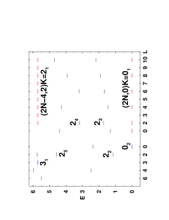
Figure 8: Left: spectrum of $\hat{H}_{cri}(\beta_{0}=\sqrt{2})$, Eq. (134), with $h_{2}=0.05$ and $N=10$. $L(K=0_{1})$ and $L(K=2_{1})$ are the solvable SU(3) states of Eq. (138a) and Eq. (138b) with $k=1$, respectively. $L=0_{2},3_{1}$ are the solvable U(5) states of Eq. (137). Right: U(5) ($n_{d}$) and SU(3) $[(\lambda,\mu)]$ decomposition for selected eigenstates of $\hat{H}_{cri}(\beta_{0}=\sqrt{2})$. Adapted from [61].

The critical Hamiltonian of Eq. (134) with $\beta_{0}=1$ is a special case of the Hamiltonian of Eq. (92), shown to have O(6)-PDS of type III. As such, it has a subset of solvable states Eq. (93), which are members of a prolate-deformed ground band, with good O(6) symmetry, $\langle\sigma\rangle=\langle N\rangle$, but broken O(5) symmetry

$$|N,\sigma=N,L\rangle\qquad E=0\qquad L=0,2,4,\ldots,2N~{}.\quad$$ (139)

In addition, $\hat{H}_{cri}(\beta_{0}=1)$ has the spherical states of Eq. (137), with good U(5) symmetry, as eigenstates. The remaining eigenstates of $\hat{H}_{cri}(\beta_{0}=1)$ shown in Fig. 9 are mixed with respect to both U(5) and O(6). Apart from the solvable U(5) states of Eq. (137), all eigenstates of $\hat{H}_{cri}(\beta_{0}=1)$ are mixed with respect to O(5) [including the solvable O(6) states of Eq. (139), as shown in the bottom right panel of Fig. 9]. It follows that the Hamiltonian has a subset of states with good U(5) symmetry and a subset of states with good O(6) but broken O(5) symmetry, and all other states are mixed with respect to both U(5) and O(6). These are precisely the required features of U(5) PDS of type I coexisting with O(6) PDS of type III.

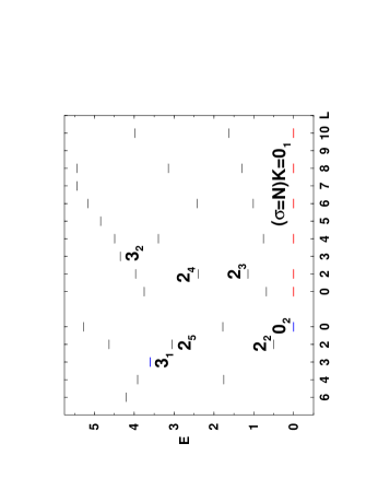
Figure 9: Upper panel: spectrum of $\hat{H}_{cri}(\beta_{0}=1)$, Eq. (134), with $h_{2}=0.05$ and $N=10$. $L(K=0_{1})$ are the solvable states of Eq. (139) with good O(6) but broken O(5) symmetry. $L=0_{2},3_{1}$ are the solvable U(5) states of Eq. (137). Bottom left panel: U(5) ($n_{d}$) and O(6) $(\sigma)$ decomposition for selected spherical and deformed eigenstates of $\hat{H}_{cri}(\beta_{0}=1)$. Bottom right panel: O(5) ($\tau$) decomposition for the $L=0,\,2$ states, Eq. (139), members of the ground band ($K=0_{1}$) of $\hat{H}_{cri}(\beta_{0}=1)$. Both states have O(6) symmetry $\sigma=N$. Adapted from [61].

In conclusion, the above results demonstrate the relevance of the PDS notion to critical-points of QPT, with phases characterized by Lie-algebraic symmetries. In the example considered, second-order critical Hamiltonians mix incompatible symmetries but preserve a common lower symmetry, resulting in a single PDS with selected quantum numbers conserved. First-order critical Hamiltonians exhibit distinct subsets of solvable states with good symmetries, giving rise to a coexistence of different PDS. The ingredients of an algebraic description of QPT is a spectrum generating algebra and an associated geometric space, formulated in terms of coherent (intrinsic) states. The same ingredients are used in the construction of Hamiltonians with PDS. These, in accord with the present discussion, can be used as tools to explore the role of partial symmetries in governing the critical behaviour of dynamical systems undergoing QPT.

7 PDS and Mixed Regular and Chaotic Dynamics

Partial dynamical symmetries can play a role not only for discrete spectroscopy but also for analyzing statistical aspects of nonintegrable systems [68, 69]. Hamiltonians with dynamical symmetry are always completely integrable [70]. The Casimir invariants of the algebras in the chain provide a set of constants of the motion in involution. The classical motion is purely regular. A dynamical symmetry-breaking is connected to nonintegrability and may give rise to chaotic motion [70, 71, 72]. Hamiltonians with PDS are not completely integrable, hence can exhibit stochastic behavior, nor are they completely chaotic, since some eigenstates preserve the symmetry exactly. Consequently, such Hamiltonians are optimally suitable to the study of mixed systems with coexisting regularity and chaos.

The dynamics of a generic classical Hamiltonian system is mixed [73]; KAM islands of regular motion and chaotic regions coexist in phase space. In the associated quantum system, if no separation between regular and irregular states is done, the statistical properties of the spectrum are usually intermediate between the Poisson and the Gaussian orthogonal ensemble (GOE) statistics. In a PDS of type I, the symmetry of the subset of solvable states is exact, yet does not arise from invariance properties of the Hamiltonian. This offers an important opportunity to study how the existence of partial (but exact) symmetries affects the dynamics of the system. If the fraction of solvable states remains finite in the classical limit, one might expect that a corresponding fraction of the phase space would consist of KAM tori and exhibit regular motion. It turns out that PDS has an even greater effect on the dynamics. It is strongly correlated with suppression (i.e., reduction) of chaos even though the fraction of solvable states approaches zero in the classical limit [68, 69].

We consider the IBM Hamiltonian of Eq. (101)

$$\hat{H}(\beta_{0}) = h_{0}\,P^{\dagger}_{0}(\beta_{0})P_{0}(\beta_{0})+h_{2}\,P^{\dagger}_{2}(\beta_{0})\cdot\tilde{P}_{2}(\beta_{0})~{}.$$ (140)

As discussed in Section 5, when $\beta_{0}=\sqrt{2}$, the Hamiltonian (140) has an SU(3)-PDS of type I. In this case, the solvable states are those of Eqs. (50)-(51). At a given spin per boson $l=L/N$, and to leading order in $1/N$, the fraction $f$ of solvable states decreases like $1/N^{2}$ with boson number. However, at a given boson number $N$, this fraction increases with $l$, a feature which is valid also for finite $N$ [68]. The classical limit of (140) is obtained [74, 75, 76] through the use of coherent states parametrized by the six complex numbers $\{\alpha_{s},\alpha_{\mu};\mu=-2,\ldots,2\}$ and taking $N\to\infty$. The classical Hamiltonian is then obtained from (140) by the substitution $s^{{\dagger}},d^{{\dagger}}_{\mu}\to\alpha_{s}^{*},\alpha_{\mu}^{*}$ and $s,d_{\mu}\to\alpha_{s},\alpha_{\mu}$ and rescaling the parameters $h_{i}\to Nh_{i}$ $(i=0,2)$. Here $1/N$ plays the role of $\hbar$.

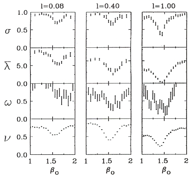
Figure 10: Classical $(\sigma,\bar{\lambda})$ and quantal $(\omega,\nu)$ measures of chaos versus $\beta_{0}$ for the Hamiltonian (140) with $h_{2}/h_{0}=7.5$. Shown are three cases with classical spins $l=0.08,\,0.4$, and $1$. The quantal calculations $(\omega,\nu)$ are done for $N=25$ bosons and spins $L=2,10$, and $25$, respectively. Notice that with increasing spin the minimum gets deeper and closer to $\beta_{0}=\sqrt{2}$. The suppression of chaos near $\beta_{0}=\sqrt{2}$ is seen both for finite $N$ through the measures $\omega,\,\nu$ and in the classical limit $N\to\infty$ through the measures $\sigma,\,\bar{\lambda}$. Adapted from [68].

To study the effect of the SU(3) PDS on the dynamics, we fix the ratio $h_{2}/h_{0}$ at a value far from the exact SU(3) symmetry (for which $h_{0}/h_{2}=1)$. We then change $\beta_{0}$ in the range $1\leq\beta_{0}\leq 2$. Classically, we determine the fraction $\sigma$ of chaotic volume and the average largest Lyapunov exponent $\bar{\lambda}$. To analyze the quantum Hamiltonian, we study spectral and transition intensity distributions. The nearest neighbors level spacing distribution is fitted by a Brody distribution, $P_{\omega}(S)=AS^{\omega}\exp(-\alpha S^{1+\omega})$, where $A$ and $\alpha$ are determined by the conditions that $P_{\omega}(S)$ is normalized to $1$ and $\langle S\rangle=1$. For the Poisson statistics $\omega=0$ and for GOE $\omega=1$, corresponding to integrable and fully chaotic classical motion [77, 78], respectively. The intensity distribution of the SU(3) E2 operator, $Q^{(2)}$ of Eq. (53), is fitted by a $\chi^{2}$ distribution in $\nu$ degrees of freedom [79], $P_{\nu}(y)=[(\nu/2\langle y\rangle)^{\nu/2}/\Gamma(\nu/2)]y^{\nu/2-1}\exp(-\nu y/2\langle y\rangle)$. For the GOE, $\nu=1$ and $\nu$ decreases as the dynamics become more regular.

Fig. 10 shows the two classical measures $\sigma$, $\bar{\lambda}$ and the two quantum measures $\omega$, $\nu$ for the Hamiltonian (140) as a function of $\beta_{0}$. The parameters of the Hamiltonian are taken to be $h_{2}/h_{0}=7.5$ and the number of bosons is $N=25$. Shown are three classical spins $l=0.08,\,0.4$ and $1$, which correspond in the quantum case to $L=2,\,10$ and $25$. All measures show a pronounced minimum which gets deeper and closer to $\beta_{0}=\sqrt{2}$ [where the partial SU(3) symmetry occurs] as the classical spin increases. This behaviour is correlated with the fraction of solvable states (at a constant $N$) being larger at higher $l$. We remark that the classical measures show a clear enhancement of the regular motion near $\beta_{0}=\sqrt{2}$ even though the fraction of solvable states vanishes as $1/N^{2}$ in the classical limit $N\to\infty$.

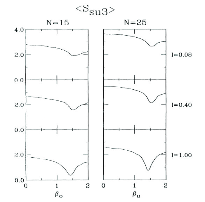
Figure 11: The average SU(3) entropy of the eigenstates of the Hamiltonian (140) (for $h_{2}/h_{0}=7.5$) versus $\beta_{0}$, for three values of the spin (per boson), $l=0.08,\,0.4$, and $1$. Left: $N=15$ bosons; right: $N=25$ bosons. Adapted from [68].

To confirm that the observed suppression of chaos is related to the SU(3) PDS, we employ the concept of an entropy [80, 81] associated with a given symmetry. To determine the SU(3) entropy, we expand any eigenstate $|\alpha LM\rangle$ in an SU(3) basis, $|\alpha LM\rangle=\sum_{(\lambda\mu),K}c^{(\alpha)}_{(\lambda,\mu)K}|(\lambda,\mu)KLM\rangle$. Denoting by $p^{(\alpha)}_{\lambda\mu}$ the probability to be in the SU(3) irrep $(\lambda,\mu)$, $p^{(\alpha)}_{\lambda\mu}=\sum_{K}|c^{(\alpha)}_{(\lambda,\mu)K}|^{2}$, the SU(3) entropy of the state $|\alpha LM\rangle$ is defined as $S^{(\alpha)}_{SU(3)}=-\sum_{\lambda,\mu}p^{(\alpha)}_{\lambda\mu}\ln p^{(\alpha)}_{\lambda\mu}$. The entropy vanishes when the state has a good SU(3) symmetry. The averaged entropy $\langle S_{{\rm SU(3)}}\rangle$ over all eigenstates is then a measure of the global SU(3) symmetry. This quantity is plotted in Fig. 11, versus $\beta_{0}$ for $N=15$ and 25 and for the same spin values (per boson) $l$ as in Fig. 10. We observe a minimum which is well correlated with the minimum in Fig. 10. The maximum SU(3) entropy is the logarithm of the number of allowed SU(3) irreps for the given $N$ and $l$. The average SU(3) entropy therefore increases with $N$. The depth of the minimum increases with $N$ and $l$ though the fraction of solvable states is smaller at $N=25$ than at $N=15$ by a factor of about 3. The existence of an SU(3) PDS seems to have an effect of increasing the SU(3) symmetry of all states, not just those with an exact SU(3) symmetry [68].

In order to better understand the strong suppression of classical chaos induced by PDS, we consider a simpler model and use its PDS to infer relationships between the classical and quantum dynamics of a Hamiltonian in a mixed KAM régime [69]. The model is based on a U(3) spectrum generating algebra and its building blocks are three types of bosons $a^{\dagger}$, $b^{\dagger}$, $c^{\dagger}$ satisfying the usual commutation relations. The nine number-conserving bilinear products of creation and destruction operators comprise the U(3) algebra. The conservation of the total boson-number $\hat{N}=\hat{n}_{a}+\hat{n}_{b}+\hat{n}_{c}$ ($\hat{n}_{a}=a^{\dagger}a$ with eigenvalue $n_{a}$ etc.) ensures that the model describes a system with only two independent degrees of freedom. All states of the model are assigned to the totally symmetric representation [N] of U(3). One of the dynamical symmetries of the model is associated with the following chain of algebras

$${\rm U(3)}\supset{\rm U(2)}\supset{\rm U(1)}$$ (141)

Here ${\rm U}(2)\equiv{\rm SU}(2)\times{\rm U}_{ab}(1)$ with a linear Casimir $\hat{n}_{ab}=\hat{n}_{a}+\hat{n}_{b}$ [which is also the generator of ${\rm U}_{ab}(1)$]. The generators of SU(2) are $\hat{J}_{+}=b^{\dagger}a$, $\hat{J}_{-}=a^{\dagger}b$, $\hat{J}_{z}=(\hat{n}_{b}-\hat{n}_{a})/2$ and its Casimir $\mbox{\boldmath$J^{2}$}=\hat{n}_{ab}(\hat{n}_{ab}+2)/4$. The subalgebra U(1) in Eq. (141) is composed of the operator $\hat{J}_{z}$. A choice of Hamiltonian with a U(2) dynamical symmetry is

$$\hat{H}_{0} = \omega_{a}a^{\dagger}a+\omega_{b}b^{\dagger}b\;\;=\;\;\hat{n}_{ab}-2A\hat{J}_{z}$$ (142)

where $\omega_{a,b}=1\pm A$, and $A$ is introduced to break degeneracies. Diagonalization of this Hamiltonian is trivial and leads to eigenenergies $E_{n_{a},n_{b}}=\omega_{a}n_{a}+\omega_{b}n_{b}$ and eigenstates $|n_{a},n_{b},n_{c}\rangle$ or equivalently $|N,J,J_{z}\rangle$ where the label $J=n_{ab}/2$ identifies the SU(2) irrep. These are states with well defined $n_{a}$, $n_{b}$ and $n_{c}=N-n_{a}-n_{b}$. To create a PDS we add the term

$$\hat{H}_{1}=b^{\dagger}(b^{\dagger}a+b^{\dagger}c+a^{\dagger}b+c^{\dagger}b)b~{},$$ (143)

which preserves the total boson number but not the individual boson numbers, so it breaks the dynamical symmetry. However, states of the form $|n_{a},n_{b}=0,n_{c}\rangle$ (or equivalently $|N,J=n_{a}/2,J_{z}=-J\rangle$ ) with $n_{a}=0,1,2,\ldots N$ are annihilated by $\hat{H}_{1}$ and therefore remain eigenstates of $\hat{H}_{0}+B\hat{H}_{1}$. The latter Hamiltonian is not an SU(2) scalar yet has a subset of $(N+1)$ “special” solvable states with SU(2) symmetry, and therefore has PDS. There is one special state per SU(2) irrep $J=n_{a}/2$ (the lowest weight state in each case) with energy $\omega_{a}n_{a}$ independent of the parameter B. Other eigenstates are mixed. Although $\hat{H}_{0}$ and $\hat{H}_{1}$ do not commute, when acting on the “special” states they satisfy

$$\Bigl{[}\hat{H}_{0}\,,\,\hat{H}_{1}\Bigr{]}|n_{a},n_{b}=0,n_{c}\rangle\;=0~{}.$$ (144)

To break the PDS we introduce a third interaction

$$\hat{H}_{2}=a^{\dagger}c+c^{\dagger}a+b^{\dagger}c+c^{\dagger}b~{}.$$ (145)

The complete Hamiltonian is then

$$\hat{H}=\hat{H}_{0}+B\,\hat{H}_{1}+C\,\hat{H}_{2}~{}.$$ (146)

For $B=C=0$ we have the full dynamical symmetry; for $B\neq 0,\,C=0$ we have partial dynamical symmetry and for $C\neq 0$ we have neither.

The classical Hamiltonian ${\cal H}_{cl}$ is obtained from (146) by replacing $(a^{\dagger},b^{\dagger},c^{\dagger})$ by complex c-numbers $(\alpha^{*},\beta^{*},\gamma^{*})$ and taking $N\rightarrow\infty$. The latter limit is obtained by rescaling ${\bar{B}}=NB$, $\alpha\rightarrow\alpha/\sqrt{N}$ etc. and considering the classical Hamiltonian per boson ${\cal H}={\cal H}_{cl}/N$. In the present model the latter has the form

$${\cal H} = {\cal H}_{0}+\bar{B}\,{\cal H}_{1}+C\,{\cal H}_{2}~{}.$$ (147)

Number conservation imposes a constraint $\alpha^{*}\alpha+\beta^{*}\beta+\gamma^{*}\gamma=1$, so that the phase space is compact and four-dimensional with a volume $2\pi^{2}$. The total number of quantum states is $(N+1)(N+2)/2$. Assigning, to leading order in $N$, one state per $(2\pi\hbar)^{2}$ volume of phase space, we identify $\hbar=1/N$, so that the classical limit is $N\rightarrow\infty$.

Figure 12: Classical ($\mu$) and quantum ($\omega$) measures of chaos [denoted by ($\bullet$) and ($\times$), respectively] versus $C$ for the Hamiltonian (146) with ${\bar{B}}=0.5$. Adapted from [69].

In all calculations reported below [69] we take $A=0.8642$ and $N=60$. As a first step, we fix ${\bar{B}}=0.5$ and vary $C$. As previously done, for the classical analysis we randomly sample the phase space and determine the fraction $\mu$ of chaotic volume (same as $\sigma$ in Fig. 10). For the quantum analysis we evaluate the energy levels, calculated the nearest neighbors level spacing distribution of the unfolded spectrum and fitted it to a Brody distribution. The latter is specified by the fit parameter $\omega$, mentioned above. As shown in Fig. 12, both of these measures indicate a suppression of chaos near $C=0$ similar to the results of Fig. 10. To appreciate the strong effect of the PDS (at $C=0$) on the underlying dynamics, it should be noted that the fraction of the solvable states $|n_{a},n_{b}=0,n_{c}\rangle$ is $2/(N+2)$, which approaches zero in the classical limit. To measure the extent to which each eigenstate $|\Psi\rangle$ has SU(2) symmetry, we define variances $\sigma_{i}^{2}=\langle\Psi|\hat{n}_{i}^{2}|\Psi\rangle-\langle\Psi|\hat{n}_{i}|\Psi\rangle^{2}$ $(i=a,b)$. A state which belongs to just one irrep of SU(2) (with well defined $J,J_{z}$) has zero variances, while a mixed state has large variances. These variances have the same physical content as the entropies considered before. It is instructive to display the average $\langle\hat{n}_{a}\rangle$ and variance of each state, as done in Fig. 13. SU(2) PDS is present in Fig. 13(a) ($B\neq 0$, $C=0$), Fig. 13(b) is a blow up of Fig 13(a), and in Fig. 13(c) the symmetry is completely broken ($C\neq 0$). In Figs. 13(a) and 13(b) we see states with zero variance. These are just the special $N+1$ states ($n_{b}=0$) discussed before, which preserve the SU(2) symmetry. In addition, we see families of states with small variance and small $\langle n_{b}\rangle$ which suggests that the presence of PDS increases the purity of states other than the special ones. By contrast, in Fig. 13(c) we see no particular structure because of the destruction of the PDS for $C\neq 0$.

Figure 13: (Left panel). The values of $\langle n_{a}\rangle$ and of the variance $\sigma_{b}$ (denoted by $\diamond$) of each eigenstate of the Hamiltonian (146). (a) ${\bar{B}}=0.5$, $C=0$ (partial dynamical symmetry). (b) a blow up of (a) with superimposed results [denoted by ($+$)] of quantum perturbation theory. The families of states with low $\sigma_{b}$ have small values of $\langle n_{b}\rangle$. (c) ${\bar{B}}=0.3$, $C=0.5$ (broken symmetry). Adapted from [69]. Figure 14: (Right panel). Poincaré sections $J_{b}$ versus $\theta_{b}$ at energy $E=1.0$. (a) ${\bar{B}}=0.5$, $C=0$ (partial dynamical symmetry). (b) a blow up of (a) with superimposed results (dashed curves) of classical perturbation theory. (c) ${\bar{B}}=0.3$, $C=0.5$ (broken symmetry). Adapted from [69].

Considerable insight is gained by examining the classical phase space structure in terms of action-angle variables $\alpha=\sqrt{J_{a}}\exp(-i\theta_{a})$, $\beta=\sqrt{J_{b}}\exp(-i\theta_{b})$ and $\gamma=\sqrt{J_{c}}=\sqrt{1-J_{a}-J_{a}}$. The $\theta_{a}=-\pi/2$ Poincaré section is shown in Fig. 14 for energy $E=1.0$. When SU(2) PDS is present (${\bar{B}}\neq 0,\,C=0$), we see in Figs. 14(a) and 14(b) a torus with $J_{b}=0$, and additional perturbed tori in its neighborhood (small $J_{b}$). This structure is absent when the symmetry is completely broken ($C\neq 0$), as shown in Fig. 14(c). The features in Fig. 14 persist also at other energies. To understand them, we recall that for ${\bar{B}}=C=0$, the Hamiltonian (147) is integrable and all trajectories wind around invariant tori. By standard torus quantization (without turning points) the actions are quantized as $J_{i}=n_{i}\hbar=n_{i}/N$ $(i=a,b)$. In the integrable limit, quantum states are associated with toroidal manifolds in phase space. In case of a partial symmetry (${\bar{B}}\neq 0,\,C=0$) we are led by analogy with Eq. (144) to seek manifolds ${\cal M}$ in phase space on which

$$\Bigl{.}\Bigl{\{}{\cal H}_{0}\,,\,{\cal H}_{1}\Bigr{\}}\Bigr{|}_{\cal M}\;=0$$ (148)

vanishes even though the Poisson bracket is not zero everywhere. In addition, we demand that $\{\{{\cal H}_{0}\,,\,{\cal H}_{1}\},{\cal H}_{0}+{\cal H}_{1}\}|_{\cal M}=0$ (in analogy to the quantum relation $[[\,H_{0},H_{1}]\,,\,H_{0}+H_{1}]|n_{a},n_{b}=0,n_{c}\rangle=0$) so that a trajectory starting on ${\cal M}$ remains on ${\cal M}$. The solution to these conditions is the manifold $J_{b}=\beta^{*}\beta=0$, which may be interpreted as a (degenerate) torus of the ${\cal H}_{0}$ Hamiltonian. It is also a stable isolated periodic orbit of ${\cal H}_{0}+\bar{B}{\cal H}_{1}$. Quantization of the torus with $J_{b}=0$ proceeds exactly as before, so we correctly predict no change in the quantum energies associated with it. The manifold ${\cal M}$ ($J_{b}=0$) is the direct classical analogue of the special quantum states $|n_{b}=0\rangle$. It refers, however, to a region of phase space of measure zero, and so cannot by itself explain the observed (global) suppression of chaos. However, as suggested by Fig. 14, the presence of PDS induces a quasi-regular region foliated by tori in the vicinity of the special torus. The dynamics on a finite measure of phase space can be understood by performing a perturbative calculation in the neighbourhood of ${\cal M}$ [69].

For the classical perturbation calculation we set $C=0$ in Eq. (147) and treat $\bar{B}$ as an expansion parameter, assuming $\bar{B}{\cal H}_{1}$ in Eq. (147) is small in the neighbourhood of the special periodic orbit. The second order correction reproduces well the perturbed tori on the Poincaré sections as shown in Fig. 14(b). The variances can be calculated in quantum perturbation theory. In Fig. 13(b) we show the results [denoted by ($+$)] of the quantum perturbation theory (to order $B^{5}$). We see that the first few families of states are reproduced. It is these states which we can recover from perturbation theory and whose approximate symmetry is induced by the symmetry of the special states.

The following physical picture emerges from the foregoing analysis. Near the special orbit, there are KAM tori, some of which are quantized. The quantum eigenstates lie on these tori, so knowing the classical variance of the actions of the tori tells us the variances of the states themselves, in the semiclassical limit. Large variances indicate the extent to which the corresponding states fail to respect the symmetry. This provides a measure for a separation of regular and irregular levels, as conceived in [82]. In the present model, the quantum states can be grouped into three classes: i) the special states, which observe the symmetry; ii) the “almost special states” which are accessible by perturbation theory; iii) the rest of the states, which are mixed. As in [73], the frontier between regular states (sets (i) and (ii) ) and irregular states (set (iii) ) is not sharp.

The above discussion illustrates the effect of PDS on the quantum and classical dynamics of a mixed system. At the quantum level, PDS by definition implies the existence of a “special” subset of states, which observe the symmetry. The PDS affects the purity of other states in the system; in particular, neighboring states, accessible by perturbation theory, possess approximately good symmetry. Analogously, at the classical level, the region of phase space near the “special” torus also has toroidal structure. As a consequence of having PDS, a finite region of phase space is regular and a finite fraction of states is approximately “special”. This clarifies the observed suppression of chaos. Based on these arguments and the above results, it is anticipated that the suppression of chaos will persist in higher dimensional systems with PDS.

8 PDS and Higher-Order Terms

In applications of algebraic modeling to dynamical systems, there is occasionally a need, based on phenomenological and/or microscopic grounds, to include higher-order terms in the Hamiltonian. For example, in the IBM, accommodating rigid triaxial shapes and describing large anharmonicities in excited bands, requires at least cubic terms in the boson Hamiltonian. From a microscopic point of view, many-body boson interactions in the IBM, are generated by the mapping of fermion pairs into bosons [83, 84] and the truncation to only monopole and quadrupole bosons, with the associated renormalization of the effective interaction in the truncated space [85, 86, 87]. From this perspective, to confine to two-body interactions in the boson space, is only a convenient lowest-order approximation.

The advantages of using higher-order terms with PDS are twofold. First, the algorithms for realizing such symmetry structures provide a systematic procedure for identifying and selecting interactions of a given order. Having at hand a selection criteria is highly desirable, since, if higher-order terms or new degrees of freedom are added, one is immediately faced with the problem of many possible interactions and a proliferation of free parameters. Second, Hamiltonians with PDS break the dynamical symmetry but retain selected subsets of solvable eigenstates with good symmetry. Such qualities are a virtue, since interactions with a PDS can be introduced, in a controlled manner, without destroying results previously obtained with a dynamical symmetry for a segment of the spectrum.

In general, the existence of quantum Hamiltonians with PDS is closely related to the order of the interaction among the constituents. IBM Hamiltonians with higher-order terms, exhibiting PDS of type II were already encountered in Subsection 3.2. In what follows, we present examples of three-body IBM Hamiltonians with U(5) and O(6) PDS of type I. Work on three-body IBM Hamiltonians with SU(3)-PDS of type I, is currently in progress and will be reported elsewhere [88].

8.1 U(5) PDS (type I) with three-body terms

The U(5) dynamical symmetry (DS) chain, ${\rm U(6)}\supset{\rm U(5)}\supset{\rm O(5)}\supset{\rm O(3)}$, and its related basis states, $|[N]\langle n_{d}\rangle(\tau)n_{\Delta}LM\rangle$, were discussed in Section 2.1. In this case, new terms show up in the DS Hamiltonian at the level of three-body interactions. The DS Hamiltonian and related spectrum now read

$$\hat{H}_{DS} = t_{1}\,\hat{n}_{d}+t_{2}\,\hat{n}_{d}^{2}+t_{3}\,\hat{n}_{d}^{3}+t_{4}\,\hat{C}_{{\rm O(5)}}+t_{5}\,\hat{n}_{d}\hat{C}_{{\rm O(5)}}+t_{6}\,\hat{C}_{{\rm O(3)}}+t_{7}\,\hat{n}_{d}\hat{C}_{{\rm O(3)}}~{},\qquad$$ (149a)

$$E_{DS} = t_{1}\,n_{d}+t_{2}\,n_{d}^{2}+t_{3}\,n_{d}^{3}+t_{4}\,\tau(\tau+3)+t_{5}\,n_{d}\tau(\tau+3)+t_{6}\,L(L+1)$$ (149b)

$$+t_{7}\,n_{d}L(L+1)~{}.$$

Terms of the form $\hat{N}\hat{C}_{G}$, with $\hat{C}_{G}$ a quadratic Casimir operator of $G={\rm U(5)},\,{\rm O(5)},\,{\rm O(3)}$, are included in $\hat{H}_{DS}$ by allowing the parameters $t_{i}$ to depend on $N$.

Table 9: Normalized three-boson U(5) tensors.

$n$	$n_{d}$	$\tau$	$n_{\Delta}$	$\ell$	$\hat{B}^{\dagger}_{[n]\langle n_{d}\rangle(\tau)n_{\Delta}\ell m}$
3	0	0	0	0	$\sqrt{\frac{1}{6}}(s^{{\dagger}})^{3}$
3	1	1	0	2	$\sqrt{\frac{1}{2}}(s^{{\dagger}})^{2}d^{{\dagger}}_{m}$
3	2	0	0	0	$\sqrt{\frac{1}{2}}s^{{\dagger}}(d^{{\dagger}}d^{{\dagger}})^{(0)}_{0}$
3	2	2	0	2	$\sqrt{\frac{1}{2}}s^{{\dagger}}(d^{\dagger}d^{\dagger})^{(2)}_{m}$
3	2	2	0	4	$\sqrt{\frac{1}{2}}s^{{\dagger}}(d^{\dagger}d^{\dagger})^{(4)}_{m}$
3	3	1	0	2	$\sqrt{\frac{5}{14}}((d^{\dagger}d^{\dagger})^{(0)}d^{\dagger})^{(2)}_{m}$
3	3	3	1	0	$\sqrt{\frac{1}{6}}((d^{\dagger}d^{\dagger})^{(2)}d^{\dagger})^{(0)}_{m}$
3	3	3	0	3	$\sqrt{\frac{7}{30}}((d^{\dagger}d^{\dagger})^{(2)}d^{\dagger})^{(3)}_{m}$
3	3	3	0	4	$\sqrt{\frac{7}{22}}((d^{\dagger}d^{\dagger})^{(2)}d^{\dagger})^{(4)}_{m}$
3	3	3	0	6	$\sqrt{\frac{1}{6}}((d^{\dagger}d^{\dagger})^{(4)}d^{\dagger})^{(6)}_{m}$

The construction of U(5)-PDS Hamiltonians with three-body terms follows the general algorithm by considering operators which annihilate, for example, the U(5) ground state, $|[N],n_{d}=\tau=L=0\rangle$. This can be accomplished by means of those U(5) tensors in Table 9 with $n_{d}\neq 0$. Several families of U(5)-PDS Hamiltonians can be defined by identifying specific three-body terms which annihilate additional U(5) basis states. One such family involves the interaction

$$\hat{V}_{0}=r_{0}\,G^{{\dagger}}_{0}G_{0}+e_{0}\left(G^{{\dagger}}_{0}K_{0}+K^{{\dagger}}_{0}G_{0}\right)$$ (150a)

$$\hat{V}_{0}|[N],n_{d}=\tau,\tau,n_{\Delta}=0,LM\rangle=0\qquad L=\tau,\tau+1,\ldots,2\tau-2,2\tau\qquad\qquad$$ (150b)

where $G^{{\dagger}}_{L,\mu}=[(d^{\dagger}d^{\dagger})^{(\rho)}d^{\dagger}]^{(L)}_{\mu}$ with $(\rho,L)=(2,0),\,(0,2),\,(2,3),\,(2,4),\,(4,6)$ and $K^{{\dagger}}_{L,\mu}=s^{{\dagger}}(d^{{\dagger}}d^{{\dagger}})^{(L)}$ with $L=0,\,2,\,4$. As shown in [89], the states of Eq. (150b) may be projected from states created by acting on the vacuum by a product of $\tau$ operators $d^{{\dagger}}_{m_{i}}$ with $m_{i}\geq 1$ for $i=1,\dots,\tau$. Hence, such states are guaranteed to contain no three $d$-boson states coupled to $L=0$ and, therefore, are annihilated by $G_{0}$. The same set of states are annihilated also by $K_{0}$, since all states with $n_{d}=\tau$ vanish under the action of $\tilde{d}\cdot\tilde{d}$ [14]. The remaining eigenstates of $\hat{V}_{0}$ (150) are mixed with respect to both U(5) and O(5). Clearly, $\hat{H}_{DS}+\hat{V}_{0}$ exhibits a U(5)-PDS of type I.

A second family of PDS Hamiltonians involves the interaction

$$\hat{V}_{2}=a_{2}\,\Pi^{(2)}\cdot U^{(2)}+\sum_{L=0,2,4}e_{L}\left(\,G^{{\dagger}}_{L}\cdot\tilde{K}_{L}+H.c.\,\right)\qquad\qquad$$ (151a)

$$\hat{V}_{2}|[N],n_{d}=\tau=L=3\rangle=0~{},$$ (151b)

where $\tilde{G}_{L,\mu}=(-1)^{\mu}G_{L,-\mu}$ and $\tilde{K}_{\mu}=(-1)^{\mu}K_{L,-\mu}$. The relation in Eq. (151b) follows from arguments similar to those given after Eq. (26). Other eigenstates of $\hat{V}_{2}$ (151) are mixed in the U(5) basis. Clearly, $\hat{H}_{DS}+\hat{V}_{2}$ exhibits a U(5)-PDS of type I.

A third family of PDS Hamiltonians involves the interaction

$$\hat{V}_{3}=r_{3}\,G^{{\dagger}}_{3}\cdot{G}_{3}+r_{0}\,G^{{\dagger}}_{0}G_{0}~{}.$$ (152)

Both terms in Eq. (152) conserve the U(5) quantum number $n_{d}$, but are not O(5) scalars. They can induce O(5) mixing subject to $\Delta\tau=2,4,6$, and their multipole form involves U(5) generators, some of which are not contained in the O(5) subalgebra. As such, and in accord with the discussion at the end of Subsection 3.2, $\hat{H}_{DS}+\hat{V}_{3}$ exhibits U(5)-PDS of type II. Since both terms in $\hat{V}_{3}$ are rotational-scalars and are diagonal in $n_{d}$, it follows that in a given $n_{d}$ multiplet, those $L$-states which have a unique $\tau$-assignment, remain pure with respect to O(5), and hence are good U(5) eigenstates. For example, the states with $n_{d}=\tau,n_{\Delta}=0,\,L=2n_{d},\,2n_{d}-2,2n_{d}-3,2n_{d}-5$, or states with $L=0$ and $n_{d}\leq 5$, or states with $L=3$ and $n_{d}\leq 8$, are all eigenstates of $\hat{V}_{3}$, diagonal in the U(5) basis. In this sense, $\hat{H}_{DS}+\hat{V}_{3}$ exhibits also O(5)-PDS of type I.

8.2 O(6) PDS (type I) with three-body terms

The O(6) dynamical symmetry (DS) chain, ${\rm U(6)}\supset{\rm O(6)}\supset{\rm O(5)}\supset{\rm O(3)}$, and its related basis states, $|[N]\langle\Sigma\rangle(\tau)n_{\Delta}LM\rangle$, were discussed in Subsection 2.3. The DS Hamiltonian is given in Eq. (64) and no new terms are added to it at the level of three-body interactions.

According to the general algorithm, the construction of interactions with O(6)-PDS of type I requires $n$-boson creation and annihilation operators with definite tensor character in the O(6) basis:

$$\hat{B}^{\dagger}_{[n]\langle\sigma\rangle(\tau)n_{\Delta}\ell m},\;\;\tilde{B}_{[n^{5}]\langle\sigma\rangle(\tau)n_{\Delta}\ell m}\equiv(-1)^{\ell-m}\left(\hat{B}^{\dagger}_{[n]\langle\sigma\rangle(\tau)n_{\Delta}\ell,-m}\right)^{\dagger}.$$ (153)

Of particular interest are tensor operators with $\sigma<n$. They have the property

$$\tilde{B}_{[n^{5}]\langle\sigma\rangle(\tau)n_{\Delta}\ell m}|[N]\langle N\rangle(\tau)n_{\Delta}LM\rangle=0,\qquad\sigma<n,$$ (154)

for all possible values of $\tau,n_{\Delta},L$ contained in the O(6) irrep $\langle N\rangle$. This is so because the action of $\tilde{B}_{[n^{5}]\langle\sigma\rangle(\tau)n_{\Delta}\ell m}$ leads to an $(N-n)$-boson state that contains the O(6) irreps $\langle\Sigma\rangle=\langle N-n-2i\rangle,\,i=0,1,\dots$ which cannot be coupled with $\langle\sigma\rangle$ to yield $\langle\Sigma\rangle=\langle N\rangle$, since $\sigma<n$. Number-conserving normal-ordered interactions that are constructed out of such tensors with $\sigma<n$ (and their Hermitian conjugates) thus have $|[N]\langle N\rangle(\tau)n_{\Delta}LM\rangle$ as eigenstates with zero eigenvalue [24].

Table 10: Normalized three-boson O(6) tensors.

$n$	$\sigma$	$\tau$	$n_{\Delta}$	$\ell$	$\hat{B}^{\dagger}_{[n]\langle\sigma\rangle(\tau)n_{\Delta}\ell m}$
3	3	0	0	0	$\sqrt{\frac{3}{16}}s^{\dagger}(d^{\dagger}d^{\dagger})^{(0)}_{0}+\sqrt{\frac{5}{48}}(s^{{\dagger}})^{3}$
3	3	1	0	2	$\sqrt{\frac{5}{112}}((d^{\dagger}d^{\dagger})^{(0)}d^{\dagger})^{(2)}_{m}+\sqrt{\frac{7}{16}}(s^{{\dagger}})^{2}d^{{\dagger}}_{m}$
3	3	2	0	2	$\sqrt{\frac{1}{2}}s^{\dagger}(d^{\dagger}d^{\dagger})^{(2)}_{m}$
3	3	2	0	4	$\sqrt{\frac{1}{2}}s^{\dagger}(d^{\dagger}d^{\dagger})^{(4)}_{m}$
3	3	3	1	0	$\sqrt{\frac{1}{6}}((d^{\dagger}d^{\dagger})^{(2)}d^{\dagger})^{(0)}_{0}$
3	3	3	0	3	$\sqrt{\frac{7}{30}}((d^{\dagger}d^{\dagger})^{(2)}d^{\dagger})^{(3)}_{m}$
3	3	3	0	4	$\sqrt{\frac{7}{22}}((d^{\dagger}d^{\dagger})^{(2)}d^{\dagger})^{(4)}_{m}$
3	3	3	0	6	$\sqrt{\frac{1}{6}}((d^{\dagger}d^{\dagger})^{(4)}d^{\dagger})^{(6)}_{m}$
3	1	0	0	0	$\sqrt{\frac{5}{16}}s^{\dagger}(d^{\dagger}d^{\dagger})^{(0)}_{0}-\sqrt{\frac{1}{16}}(s^{{\dagger}})^{3}$
3	1	1	0	2	$\sqrt{\frac{5}{16}}((d^{\dagger}d^{\dagger})^{(0)}d^{\dagger})^{(2)}_{m}-\sqrt{\frac{1}{16}}(s^{{\dagger}})^{2}d^{{\dagger}}_{m}$

As shown in Subsection 2.3, there is one two-boson operator $P^{\dagger}_{0}=d^{\dagger}\cdot d^{\dagger}-(s^{\dagger})^{2}$, Eq. (66), with $\sigma<n=2$, which gives rise to an O(6)-invariant interaction, $P^{{\dagger}}_{0}P_{0}$, related to the completely solvable Casimir operator of O(6), Eq. (71). On the other hand, from Table 10, one recognizes two three-boson O(6) tensors with $\sigma<n=3$

$$\hat{B}^{\dagger}_{[3]\langle 1\rangle(1)0;2m}=\textstyle{\frac{1}{4}}P^{{\dagger}}_{0}d^{\dagger}_{m},\quad\hat{B}^{\dagger}_{[3]\langle 1\rangle(0)0;00}=\textstyle{\frac{1}{4}}P^{{\dagger}}_{0}s^{\dagger},$$ (155)

and from these one can construct the interactions with an O(6) PDS. The only three-body interactions that are partially solvable in O(6) are thus $P^{{\dagger}}_{0}\hat{n}_{s}P_{0}$ and $P^{{\dagger}}_{0}\hat{n}_{d}P_{0}$. Since the combination $P^{{\dagger}}_{0}(\hat{n}_{s}+\hat{n}_{d})P_{0}=(\hat{N}-2)P^{{\dagger}}_{0}P_{0}$ is completely solvable in O(6), there is only one genuine partially solvable three-body interaction which can be chosen as $P^{{\dagger}}_{0}\hat{n}_{s}P_{0}$, with tensorial components $\sigma=0,\,2$. The O(6)-DS spectrum

Figure 15: Observed spectrum of ¹⁹⁶Pt compared with the calculated spectra of $\hat{H}_{\rm DS}$ (64), with O(6) dynamical symmetry (DS), and of $\hat{H}_{\rm PDS}$ (157) with O(6) partial dynamical symmetry (PDS). The parameters in $\hat{H}_{\rm DS}$ $(\hat{H}_{\rm PDS})$ are $h_{0}=43.6\,(30.7)$, $B=44.0\,(44.0)$, $C=17.9\,(17.9)$, and $\eta=0\,(8.7)$ keV. The boson number is $N=6$ and $\Sigma$ is an O(6) label. Adapted from [24].

$$E_{\rm DS} = 4h_{0}\,(N-v+2)v+B\,\tau(\tau+3)+\,C\,L(L+1)~{},$$ (156)

resembles that of a $\gamma$-unstable deformed rotovibrator, where states are arranged in bands with O(6) quantum number $\Sigma=N-2v$, $(v=0,1,2,\ldots)$. The O(5) and O(3) terms in the dynamical symmetry Hamiltonian, $\hat{H}_{\rm DS}$ (64), govern the in-band rotational splitting. A comparison with the experimental spectrum and E2 rates of ¹⁹⁶Pt is shown in Fig. 15 and Table 11.

Table 11: Observed (EXP) and calculated B(E2) values (in $e^{2}{\rm b}^{2}$) for ¹⁹⁶Pt. For both the exact (DS) and partial (PDS) O(6) dynamical symmetry calculations, the E2 operator is that of Eq. (6) with $e_{B}=0.151$ $e$b and $\chi=0.29$. Only the state $0^{+}_{3}$ has a mixed O(6) character. Adapted from [24].

Transition	EXP	DS	PDS	Transition	EXP	DS	PDS
$2^{+}_{1}\rightarrow 0^{+}_{1}$	0.274 (1)	0.274	0.274	$2^{+}_{3}\rightarrow 0^{+}_{2}$	0.034 (34)	0.119	0.119
$2^{+}_{2}\rightarrow 2^{+}_{1}$	0.368 (9)	0.358	0.358	$2^{+}_{3}\rightarrow 4^{+}_{1}$	0.0009 (8)	0.0004	0.0004
$2^{+}_{2}\rightarrow 0^{+}_{1}$	3.10-8(3)	0.0018	0.0018	$2^{+}_{3}\rightarrow 2^{+}_{2}$	0.0018 (16)	0.0013	0.0013
$4^{+}_{1}\rightarrow 2^{+}_{1}$	0.405 (6)	0.358	0.358	$2^{+}_{3}\rightarrow 0^{+}_{1}$	0.00002 (2)	0	0
$0^{+}_{2}\rightarrow 2^{+}_{2}$	0.121 (67)	0.365	0.365	$6^{+}_{2}\rightarrow 6^{+}_{1}$	0.108 (34)	0.103	0.103
$0^{+}_{2}\rightarrow 2^{+}_{1}$	0.019 (10)	0.003	0.003	$6^{+}_{2}\rightarrow 4^{+}_{2}$	0.331 (88)	0.221	0.221
$4^{+}_{2}\rightarrow 4^{+}_{1}$	0.115 (40)	0.174	0.174	$6^{+}_{2}\rightarrow 4^{+}_{1}$	0.0032 (9)	0.0008	0.0008
$4^{+}_{2}\rightarrow 2^{+}_{2}$	0.196 (42)	0.191	0.191	$0^{+}_{3}\rightarrow 2^{+}_{2}$	$<0.0028$	0.0037	0.0028
$4^{+}_{2}\rightarrow 2^{+}_{1}$	0.004 (1)	0.001	0.001	$0^{+}_{3}\rightarrow 2^{+}_{1}$	$<0.034$	0	0
$6^{+}_{1}\rightarrow 4^{+}_{1}$	0.493 (32)	0.365	0.365

The O(6)-DS limit is seen to provide a good description for properties of states in the ground band $(\Sigma=N)$. This observation was the basis of the claim [90] that the O(6)-DS is manifested empirically in ¹⁹⁶Pt. However, the resulting fit to energies of excited bands is quite poor. The $0^{+}_{1}$, $0^{+}_{3}$, and $0^{+}_{4}$ levels of ¹⁹⁶Pt at excitation energies 0, 1403, 1823 keV, respectively, are identified as the bandhead states of the ground $(v=0)$, first- $(v=1)$ and second- $(v=2)$ excited vibrational bands [90]. Their empirical anharmonicity, defined by the ratio $R=E(v=2)/E(v=1)-2$, is found to be $R=-0.70$. In the O(6)-DS limit these bandhead states have $\tau=L=0$ and $\Sigma=N,N-2,N-4$, respectively. The anharmonicity $R=-2/(N+1)$, as calculated from Eq. (156), is fixed by $N$. For $N=6$, which is the appropriate boson number for ¹⁹⁶Pt, the O(6)-DS value is $R=-0.29$, which is in marked disagreement with the empirical value. A detailed study of double-phonon excitations within the IBM, has concluded that large anharmonicities can be incorporated only by the inclusion of at least cubic terms in the Hamiltonian [91]. In the IBM there are 17 possible three-body interactions [8]. One is thus confronted with the need to select suitable higher-order terms that can break the DS in excited bands but preserve it in the ground band. On the basis of the preceding discussion this can be accomplished by the following Hamiltonian with O(6)-PDS [24]

$$\hat{H}_{\rm PDS}=\hat{H}_{\rm DS}+\eta\,P^{{\dagger}}_{0}\hat{n}_{s}P_{0},$$ (157)

where the terms are defined in Eqs. (64) and (155). The spectrum of $\hat{H}_{\rm PDS}$ is shown in Fig. 15. The states belonging to the $\Sigma=N=6$ multiplet remain solvable with energies given by the same DS expression, Eq. (156). States with $\Sigma<6$ are generally admixed but agree better with the data than in the DS calculation. For example, the bandhead states of the first- (second-) excited bands have the O(6) decomposition $\Sigma=4$: $76.5\%\,(19.6\%)$, $\Sigma=2$: $16.1\%\,(18.4\%)$, and $\Sigma=0$: $7.4\%\,(62.0\%)$. Thus, although the ground band is pure, the excited bands exhibit strong O(6) breaking. The calculated O(6)-PDS anharmonicity for these bands is $R=-0.63$, much closer to the empirical value, $R=-0.70$. It should be emphasized that not only the energies but also the wave functions of the $\Sigma=N$ states remain unchanged when the Hamiltonian is generalized from DS to PDS. Consequently, the E2 rates for transitions among this class of states are the same in the DS and PDS calculations. Thus, the additional three-body term in the Hamiltonian (157), does not spoil the good O(6)-DS description for this segment of the spectrum. This is evident in Table 11 where most of the E2 data concern transitions between $\Sigma=N=6$ states. Only transitions involving states from excited bands (e.g., the $0^{+}_{3}$ state in Table 11) can distinguish between DS and PDS. Unfortunately, such interband E2 rates are presently poorly known experimentally. Their measurement is highly desirable for further testing the O(6)-PDS wave functions.

9 PDS and Coupled Systems

So far the notion of partial dynamical symmetries was presented in the framework of algebraic models involving only one species of constituent particle. It is of great interest to extend this notion to the case of coupled systems involving two (or more) species of particles. In this case, the appropriate spectrum generating algebra, $G_{1}\times G_{2}$, contains the direct product of the two algebraic structures for systems 1 and 2.

An example of such a coupled system is the proton-neutron version of the interacting boson model (IBM-2) [8, 92, 93]. The building blocks of the model are monopole and quadrupole bosons, $\{s^{{\dagger}}_{\rho},\,d^{{\dagger}}_{\rho\mu}\}$, of proton type ($\rho=\pi$) and of neutron type $(\rho=\nu$), representing pairs of identical valence nucleons. Number conserving bilinear combinations of operators in each set comprise the ${\rm U}_{\rho}(6)$ algebra as in the IBM-1, Eq. (1), and bosons of different types commute. Since the separate proton- and neutron- boson numbers, $\hat{N}_{\pi}$ and $\hat{N}_{\nu}$, are conserved, the appropriate spectrum generating algebra of the model is ${\rm U}_{\pi}(6)\times{\rm U}_{\nu}(6)$. Subalgebras can be constructed with the aid of the individual subalgebras, ${\rm U}_{\rho}(5),\,{\rm SU}_{\rho}(3),\,{\rm O}_{\rho}(6),\,{\rm O}_{\rho}(5),\,{\rm O}_{\rho}(3)$. For instance, for a given algebra $G_{\rho}$, with generators $g_{\rho}$, there is a combined algebra $G_{\pi+\nu}$, with generators $g_{\pi}+g_{\nu}$. The dynamical symmetries of the IBM-2 are obtained by identifying the lattices of embedded algebras starting with ${\rm U}_{\pi}(6)\times{\rm U}_{\nu}(6)$ and ending with the symmetry algebra ${\rm O}_{\pi+\nu}(3)$.

A new aspect in coupled systems is the occurrence of states which are not symmetric with respect to interchange of the two constituents. This is clearly seen in the reduction

$$\begin{array}[]{ccc}{\rm U}_{\pi}(6)\times{\rm U}_{\nu}(6)&\supset&{\rm U}_{\pi+\nu}(6)\\ \downarrow&&\downarrow\\ \,[N_{\pi}]\times[N_{\nu}]&&[N_{1},N_{2}]\end{array}~{}.$$ (161)

For a given irrep of ${\rm U}_{\pi}(6)\times{\rm U}_{\nu}(6)$, characterized by $N_{\pi}$ and $N_{\nu}$, the allowed irreps of ${\rm U}_{\pi+\nu}(6)$ are $[N_{1},N_{2}]=[N_{\pi}+N_{\nu}-k,k]$, where $k=0,1,\ldots,{\rm min}\{N_{\pi},\,N_{\nu}\}$. States in the irreps with $N_{2}\neq 0$ ($k\neq 0$) are not symmetric with respect to $\pi$ and $\nu$ bosons. One of the successes of the IBM-2 has been the empirical discovery of such low-lying mixed symmetry states in nuclei, in which valence protons and neutrons move out of phase. A complete listing of all possible partial dynamical symmetries (PDS) of the IBM-2 is outside the scope of the present review. In what follows, we present a sample of such symmetry structures, illuminating new features of PDS in coupled systems.

Coupled algebraic structure, $G_{1}\times G_{2}$, can involve also fermionic algebras, as well as Bose-Fermi algebras. An example of the latter is the interacting boson-fermion model (IBFM) [9], used for describing odd-mass nuclei and broken fermion-pairs in even-even nuclei. The model incorporates collective (bosonic) and quasi-particle (fermionic) degrees of freedom, and the associated spectrum generating algebra is ${\rm U}_{B}(6)\times{\rm U}_{F}(m)$. Here ${\rm U}_{B}(6)$ and ${\rm U}_{F}(m)$ are the boson and fermion algebras respectively, and $m=\sum_{i}(2j_{i}+1)$ is the dimension of the single-particle space ($j_{i}$ are the angular momenta of the occupied shell-model orbits). Bose-Fermi symmetries correspond to dynamical symmetries of ${\rm U}_{B}(6)\times{\rm U}_{F}(m)$. Supersymmetry corresponds to a further embedding of the Bose-Fermi symmetry into a graded Lie algebra ${\rm U}(6/m)\supset{\rm U_{B}}(6)\times{\rm U_{F}}(m)$. Partial Bose-Fermi symmetries and partial supersymmetries have not been considered in detail so far. There are initial hints that such a structure can occur in the IBFM [94], however, an in-depth systematic study is called for.

9.1 F-spin and selected PDS in the IBM-2

The proton-neutron degrees of freedom are naturally reflected in the IBM-2 via an ${\rm SU}_{F}(2)$ F-spin algebra [92] with generators

$$\hat{F}_{+}=s^{\dagger}_{\pi}s_{\nu}+d^{\dagger}_{\pi}\cdot\tilde{d}_{\nu}\;\;,\;\;\hat{F}_{-}=(\hat{F}_{+})^{\dagger}\;\;,\;\;\hat{F}_{0}=(\hat{N}_{\pi}-\hat{N}_{\nu})/2~{}.$$ (162)

These generators commute with the total boson number operator, $\hat{N}=\hat{N}_{\pi}+\hat{N}_{\nu}$, which is a ${\rm U}_{N}(1)$ generator. The basic F-spin doublets are $(s^{\dagger}_{\pi},s^{\dagger}_{\nu})$, and $(d^{\dagger}_{\pi\mu},d^{\dagger}_{\nu\mu})$, with F-spin projection +1/2 ($-$1/2) for proton (neutron) bosons. The algebras ${\rm SU}_{F}(2)\times{\rm U}_{N}(1)$ (162) and ${\rm U}_{\pi+\nu}(6)$ (161) commute and obey a duality relationship, in the sense that their irreps are related by $F=(N_{1}-N_{2})/2=(N_{\pi}+N_{\nu})/2-k$ and $N=N_{1}+N_{2}=N_{\pi}+N_{\nu}$. In a given nucleus, with fixed $N_{\pi}$, $N_{\nu}$, all states have the same value of $F_{0}=(N_{\pi}-N_{\nu})/2$, while the allowed values of the F-spin quantum number F range from $|F_{0}|$ to $F_{max}\equiv(N_{\pi}+N_{\nu})/2\equiv N/2$ in unit steps. F-spin characterizes the $\pi$-$\nu$ symmetry properties of IBM-2 states. States with maximal F-spin, $F\equiv F_{max}$, are fully symmetric and correspond to the IBM-1 states with only one type of bosons [8]. There are several arguments, e.g., the empirical success of IBM-1, the identification of F-spin multiplets [95, 96, 97, 98] (series of nuclei with constant $F$ and varying $F_{0}$ with nearly constant excitation energies), and weakness of M1 transitions, which lead to the belief that low lying collective states have predominantly $F=F_{max}$ [99]. States with $F<F_{max}$, correspond to ‘mixed-symmetry’ states [100], most notably, the orbital magnetic dipole scissors mode [101] has by now been established experimentally as a general phenomena in deformed even-even nuclei [102].

Table 12: Energies (in MeV) of $2^{+}$ levels of the ground ($g$), $\gamma$ and $\beta$ bands in F-spin multiplets. The mass numbers are $A=132+4F$. Adapted from [103].

F	Energy	ADy	A+4Er	A+8Yb	A+12Hf	A+16W	A+20Os
6	$E(2^{+}_{g})$	0.14	0.13	0.12	0.12	0.12	0.14
	$E(2^{+}_{\gamma})$	0.89	0.85	0.86	0.88		0.86
	$E(2^{+}_{\beta})$	0.83	1.01	1.07	1.06		0.74
13/2	$E(2^{+}_{g})$	0.10	0.10	0.10	0.10	0.11	0.13
	$E(2^{+}_{\gamma})$	0.95	0.90	0.93	0.96
	$E(2^{+}_{\beta})$	1.09	1.17	1.14	0.99
7	$E(2^{+}_{g})$	0.09	0.09	0.09	0.10	0.11	0.13
	$E(2^{+}_{\gamma})$	0.97	0.86	0.98	1.08		0.87
	$E(2^{+}_{\beta})$	1.35	1.31	1.23	0.95		0.83
15/2	$E(2^{+}_{g})$	0.08	0.08	0.08	0.09	0.11
	$E(2^{+}_{\gamma})$	0.89	0.79	1.15	1.23	1.11
	$E(2^{+}_{\beta})$	1.45	1.53	1.14	0.90	1.08
8	$E(2^{+}_{g})$	0.07	0.08	0.08	0.09
	$E(2^{+}_{\gamma})$	0.76	0.82	1.47	1.34
	$E(2^{+}_{\beta})$		1.28	1.12	1.23
17/2	$E(2^{+}_{g})$	0.08	0.08	0.08
	$E(2^{+}_{\gamma})$	0.86	0.93	1.63
	$E(2^{+}_{\beta})$	1.21	0.96	1.56

Various procedures have been proposed to estimate the F-spin purity of low lying states [99]. In the majority of analyses, based on M1 transitions (which should vanish between pure $F=F_{max}$ states), magnetic moments and energy systematics of mixed-symmetry states, the F-spin admixtures in low lying states are found to be of a few percents ($<10\%$), typically $2\%-4\%$ [99]. In spite of its appeal, however, F-spin cannot be an exact symmetry of the Hamiltonian. The assumption of F-spin scalar Hamiltonians is at variance with the microscopic interpretation of the IBM-2, which necessitates different effective interactions between like and unlike nucleons [17]. Furthermore, if F-spin was a symmetry of the Hamiltonian, then all states would have good F-spin and would be arranged in F-spin multiplets. Experimentally this is not case. As noted in an analysis [96, 97] of rare earth nuclei, the ground bands are in F-spin multiplets, whereas the vibrational $\beta$ bands and some $\gamma$ bands do not form good F-spin multiplets. The empirical situation in the deformed Dy-Os region is portrayed in Table 12 and Fig. 16. From Table 12 it is seen that, for $F>13/2$, the energies of the $L=2^{+}$ members of the $\gamma$ bands vary fast in the multiplet and not always monotonically. The variation in the energies of the $\beta$ bands is large and irregular. Thus both microscopic and empirical arguments rule out F-spin invariance of the Hamiltonian. F-spin can at best be an approximate quantum number which is good only for a selected set of states while other states are mixed. We are thus confronted with a situation of having ‘special states’ endowed with a good symmetry which does not arise from invariance of the Hamiltonian. These are precisely the characteristics of a partial symmetry for which a non-scalar Hamiltonian produces a subset of special (at times solvable) states with good symmetry. In what follows we present IBM-2 Hamiltonians with F-spin as a partial symmetry [103]. The construction process is similar to that employed in Section 5 for obtaining partially-solvable IBM-1 Hamiltonians. Predictions of F-spin PDS are then confronted with empirical data.

Figure 16: Experimental levels of the ground $\gamma$ and $\beta$ bands in an F-spin multiplet $F=6$ of rare earth nuclei. Levels shown are up to $L=8^{+}_{g}$ for the ground band, $L=2^{+}_{\gamma},3^{+}_{\gamma}$ for the $\gamma$ band (diamonds connected by dashed lines) and $L=0^{+}_{\beta},2^{+}_{\beta}$ for the $\beta$ band (squares connected by dotted lines). Adapted from [103].

The ground band in the IBM-2 is represented by an intrinsic state which is a product of a proton condensate and a rotated neutron condensate with $N_{\pi}$ and $N_{\nu}$ bosons, respectively [104]. It depends on the quadrupole deformations, $\beta_{\rho},\gamma_{\rho}$, ($\rho=\pi,\nu$) of the proton-neutron equilibrium shapes and on the relative orientation angles $\Omega$ between them. For $\beta_{\rho}>0$, the intrinsic state is deformed and members of the rotational ground-state band are obtained from it by projection. It has been shown in [105] that the intrinsic state will have a well defined F-spin, $F=F_{max}$, when the proton-neutron shapes are aligned and with equal deformations. The conditions ($\beta_{\pi}=\beta_{\nu}$,$\gamma_{\pi}=\gamma_{\nu}$, $\Omega=0$) are weaker than the conditions for F-spin invariance, which makes it possible for a non-F-scalar IBM-2 Hamiltonian to have an equilibrium intrinsic state with pure F-spin. Focusing on the most likely situation, namely, aligned axially symmetric (prolate) deformed shapes ($\beta_{\rho}=\beta$, $\gamma_{\rho}=\Omega=0$), the equilibrium deformed intrinsic state for the ground band with $F=F_{max}$ has the form

$$|c;K=0\rangle \equiv |N_{\pi},N_{\nu}\rangle=(N_{\pi}!N_{\nu}!)^{-1/2}(b^{\dagger}_{c,\pi})^{N_{\pi}}\,(b^{\dagger}_{c,\nu})^{N_{\nu}}|0\rangle~{},$$

$$b^{\dagger}_{c,\rho} = (1+\beta^{2}\,)^{-1/2}(\,s^{\dagger}_{\rho}+\beta\,d^{\dagger}_{\rho,0}\,)~{},$$ (163)

where $K$ denotes the angular momentum projection on the symmetry axis.

The construction of partially-solvable IBM-2 Hamiltonian with F-spin partial symmetry, can be accomplished by means of the following boson-pair operators [103]

$$\begin{array}[]{ll}R^{\dagger}_{\rho,0}=d^{\dagger}_{\rho}\cdot d^{\dagger}_{\rho}-\beta^{2}(s^{\dagger}_{\rho})^{2},&R^{\dagger}_{(\pi\nu),0}=\sqrt{2}\,(\,d^{\dagger}_{\pi}\cdot d^{\dagger}_{\nu}-\beta^{2}s^{\dagger}_{\pi}s^{\dagger}_{\nu}\,)\\[2.84526pt] R^{\dagger}_{\rho,2}=\sqrt{2}\,\beta\,s^{\dagger}_{\rho}d^{\dagger}_{\rho}+\sqrt{7}(d^{\dagger}_{\rho}d^{\dagger}_{\rho})^{(2)},&R^{\dagger}_{(\pi\nu),2}=\beta(\,s^{\dagger}_{\pi}d^{\dagger}_{\nu}+s^{\dagger}_{\nu}d^{\dagger}_{\pi}\,)+\sqrt{14}(d^{\dagger}_{\pi}d^{\dagger}_{\nu})^{(2)}\\[2.84526pt] W^{\dagger}_{L}=(d^{\dagger}_{\pi}d^{\dagger}_{\nu})^{(L)}\;\;(L=1,3),&W^{\dagger}_{2}=s^{\dagger}_{\pi}d^{\dagger}_{\nu}-s^{\dagger}_{\nu}d^{\dagger}_{\pi}\end{array}\qquad$$ (167)

The $R^{\dagger}_{\rho,L}$ pairs ($\rho=\pi,\nu$) are the same $L=0,2$ pairs of Eq. (98) and the $\pi$-$\nu$ pair, $R^{\dagger}_{(\pi\nu),L}$, completes the set to form an $F$-spin vector. Altogether, the $R^{\dagger}_{i,L}$ ($L=0,2$) are boson pairs with $F=1$ and $(F_{0}=1,0,-1)\leftrightarrow[i=\pi,(\pi\nu),\nu]$. The $W^{\dagger}_{L}$ $(L=1,2,3)$ are F-spin scalar ($F=0$) $\pi$-$\nu$ boson pairs. All these operators satisfy

$$R_{i,L^{\prime}\mu}|c;K=0\rangle = 0~{},$$ (168a)

$$W_{L^{\prime}\mu}|c;K=0\rangle = 0~{},$$ (168b)

or equivalently,

$$R_{i,L^{\prime}\mu}|c;\,[N_{\pi}],[N_{\nu}],\,F=F_{max},LM\rangle = 0~{},$$ (169a)

$$W_{L^{\prime}\mu}|c;\,[N_{\pi}],[N_{\nu}],\,F=F_{max},LM\rangle = 0~{}.$$ (169b)

The states in Eq. (169) are those obtained by ${\rm O}_{\pi+\nu}(3)$ projection from the intrinsic state (163). Since the angular momentum projection operator is an F-spin scalar, the projected states of good L will also have good $F=F_{max}$. Following the general algorithm, an IBM-2 Hamiltonian with partial F-spin symmetry can be constructed as

$$\hat{H} = \sum_{i}\sum_{L=0,2}A^{(i)}_{L}R^{\dagger}_{i,L}\cdot\tilde{R}_{i,L}+\sum_{L=1,2,3}B_{L}W^{\dagger}_{L}\cdot\tilde{W}_{L}+C_{2}\Bigl{[}R^{\dagger}_{(\pi\nu),2}\cdot\tilde{W}_{2}+H.c.\Bigr{]}~{},\qquad\;\;\;$$ (170)

where $\tilde{R}_{i,L,\mu}=(-1)^{\mu}R_{i,L,-\mu}$, $\tilde{W}_{L,\mu}=(-1)^{\mu}W_{L,-\mu}$. The above Hamiltonian is an F-spin scalar only when $A^{(\pi)}_{L}=A^{(\nu)}_{L}=A^{(\pi\nu)}_{L}\,(L=0,2)$ and $C_{2}=0$. Nevertheless, the relations of Eqs. (168)-(169) ensure that it has a solvable zero-energy band with good F-spin for any choice of parameters $A^{(i)}_{L},\,B_{L},\,C_{2}$ and any $N_{\pi},N_{\nu}$. When $A^{(i)}_{L},\,B_{L},\,A^{(\pi\nu)}_{2}B_{2}-(C_{2})^{2}\geq 0$, $\hat{H}$ (170) becomes positive-definite and the solvable states form its ground band. We thus have a non-F-spin scalar Hamiltonian with a solvable (degenerate) ground band with $F=F_{max}$. The degeneracy can be lifted by adding to the Hamiltonian ${\rm O}_{\pi+\nu}(3)$ rotation terms which produce $L(L+1)$ type splitting but do not affect the wave functions. States in other bands can be mixed with respect to F-spin, hence the F-spin symmetry of $\hat{H}$ is partial. $\hat{H}$ trivially commutes with $\hat{F}_{0}$ but not with $\hat{F}_{\pm}$. However, $[\,\hat{H},\hat{F}_{\pm}\,]|c;K=0\rangle=0$ does hold and, therefore, $\hat{H}$ will yield F-spin multiplets for members of ground bands. On the other hand, states in other bands can have F-spin admixtures and are not compelled to form F-spin multiplets. These features which arise from the partial F-spin symmetry of the Hamiltonian are in line with the empirical situation as discussed above and as depicted in Table 12 and Fig. 16. It should be noted that the partial F-spin symmetry of $\hat{H}$ holds for any choice of parameters in Eq. (170). In particular, one can incorporate realistic shell-model based constraints, by choosing the $A^{(\rho)}_{2}$ ($\rho=\pi,\nu$) terms (representing seniority-changing interactions between like nucleons), to be small. For the special choice $A^{(i)}_{2}=C_{2}=0$ and $B_{1}=B_{3}$, $\hat{H}$ of Eq. (170) becomes ${\rm O}_{\pi+\nu}(5)$-scalar which commutes, therefore, with the ${\rm O}_{\pi+\nu}(5)$ projection operator and hence produces F-spin multiplets with good ${\rm O}_{\pi+\nu}(5)$ symmetry. Such multiplets were reported in the Yb-Os region of $\gamma$-soft nuclei [98].

The same conditions ($\beta_{\rho}=\beta$, $\gamma_{\rho}=\Omega=0$) which resulted in $F=F_{max}$ for the condensate of Eq. (163), ensure also $F=F_{max}-1$ for the intrinsic state representing the scissors band

$$|sc;K=1\rangle = \Gamma^{\dagger}_{sc}|N_{\pi}-1,N_{\nu}-1\rangle~{},$$

$$\Gamma^{\dagger}_{sc} = b^{\dagger}_{c,\pi}d^{\dagger}_{\nu,1}-d^{\dagger}_{\pi,1}b^{\dagger}_{c,\nu}~{}.$$ (171)

Here $\Gamma^{\dagger}_{sc}$ is a $F=0$ deformed boson pair whose action on the condensate with $(N-2)$ bosons produces the scissors mode excitation. The states of good $L$ projected from this intrinsic state, $|sc;\,[N_{\pi}],[N_{\nu}],\,F=F_{max}-1,LM\rangle$ retain the F-spin quantum number, $F=F_{max}-1$. Futhermore, it can be shown that the operators $R^{{\dagger}}_{i,L\mu}$ of Eq. (167) satisfy

$$R_{i,L^{\prime}\mu}|sc;K=1\rangle=0~{},$$ (172a)

$$R_{i,L^{\prime}\mu}|sc;\,[N_{\pi}],[N_{\nu}],\,F=F_{max}-1,LM\rangle=0~{}.$$ (172b)

Consequently, the scissors intrinsic state (171) and corresponding $L$-projected states are exact eigenstates of the following Hamiltonian, obtained from Eq. (170) for the special choice $C_{2}=0$ and $B_{1}=B_{3}=2B_{2}\equiv 2B$

$$\hat{H}^{\prime} = \sum_{i}\sum_{L=0,2}A^{(i)}_{L}R^{\dagger}_{i,L}\cdot\tilde{R}_{i,L}+B\hat{{\cal M}}_{\pi\nu}~{}.$$ (173)

The last term in Eq. (173) is the Majorana operator [8], with eigenvalues $k(N-k+1)$ for states with $F=F_{max}-k$. It is related to the total F-spin operator and the quadratic Casimir operator of ${\rm U}_{\pi+\nu}(6)$ by ${\hat{\cal M}}_{\pi\nu}=[\,\hat{N}(\hat{N}+2)/4-\mbox{\boldmath$F^{2}$}\,]=[\,\hat{N}(\hat{N}+5)-\hat{C}_{2}[{\rm U}_{\pi+\nu}(6)]\,]/2$. Adding an ${\rm O}_{\pi+\nu}(3)$ rotation term we obtain the following Hamiltonian with F-spin PDS

$$\hat{H}_{PDS}=\hat{H}^{\prime}+C\,\hat{C}_{2}[{\rm O}_{\pi+\nu}(3)]=\hat{H}_{DS}+\sum_{i}\sum_{L=0,2}A^{(i)}_{L}R^{\dagger}_{i,L}\cdot\tilde{R}_{i,L}~{}.$$ (174)

Here $\hat{H}_{DS}$ contains the Majorana and ${\rm O}_{\pi+\nu}(3)$ terms, associated with the dynamical symmetry chain ${\rm U}_{\pi+\nu}(6)\supset{\rm O}_{\pi+\nu}(3)$. $\hat{H}_{PDS}$ (174) has subsets of solvable states which form the $K=0$ ground band with $F=F_{max}$,

$$|c;\,[N_{\pi}],[N_{\nu}],\,F=F_{max},LM\rangle\;\;\;\;\;L=0,2,4,\ldots,2N$$ (175a)

$$E_{g}(L)=C\,L(L+1)~{},$$ (175b)

and the $K=1$ scissors band with $F=F_{max}-1$

$$|sc;\,[N_{\pi}],[N_{\nu}],\,F=F_{max}-1,LM\rangle\;\;\;\;\;L=1,2,3,\ldots,2N-1$$ (176a)

$$E_{sc}(L)=B\,N+C\,L(L+1)~{}.$$ (176b)

It follows that for such Hamiltonians, both the ground and scissors band have good F-spin and have the same moment of inertia. The latter derived property is in agreement with the conclusions of a comprehensive analysis of the scissors mode in heavy even-even nuclei [106], which concluded that, within the experimental precisions ($\sim$ 10%), the moment of inertia of the scissors mode are the same as that of the ground band. It is the partial F-spin symmetry of the Hamiltonian (174) which is responsible for the common signatures of collectivity in these two bands.

Table 13: The ratio $R=\sum B(M1)\uparrow/(C_{F,F_{0}})^{2}$ for members of F-spin multiplets. Here $\sum B(M1)\uparrow$ denotes the experimental summed M1 strength to the scissors mode [108, 109] and $C_{F,F_{0}}=(F,F_{0};1,0|F-1,F_{0})$. Adapted from [103].

Nucleus	$F$	$F_{0}$	$\sum B(M1)\uparrow$ $[\mu_{N}^{2}]$	$(C_{F,F_{0}})^{2}$	$R$
148Nd	4	1	0.78 (0.07)	5/12	1.87 (0.17)
148Sm		2	0.43 (0.12)	1/3	1.29 (0.36)
150Nd	9/2	1/2	1.61 (0.09)	4/9	3.62 (0.20)
150Sm		3/2	0.92 (0.06)	2/5	2.30 (0.15)
154Sm	11/2	1/2	2.18 (0.12)	5/11	4.80 (0.26)
154Gd		3/2	2.60 (0.50)	14/33	6.13 (1.18)
160Gd	7	0	2.97 (0.12)	7/15	6.36 (0.26)
160Dy		1	2.42 (0.18)	16/35	5.29 (0.39)
162Dy	15/2	1/2	2.49 (0.13)	7/15	5.34 (0.28)
166Er		$-1/2$	2.67 (0.19)	7/15	5.72 (0.41)
164Dy	8	0	3.18 (0.15)	8/17	6.76 (0.32)
168Er		$-1$	3.30 (0.12)	63/136	7.12 (0.26)
172Yb		$-2$	1.94 (0.22)a)	15/34	4.40 (0.50)
170Er	17/2	$-3/2$	2.63 (0.16)	70/153	5.75 (0.35)
174Yb		$-5/2$	2.70 (0.31)	66/153	6.26 (0.72)

^a) The low value of $\sum B(M1)\uparrow$ for ¹⁷²Yb has been attributed to experimental deficiencies [102].             

The Hamiltonian $\hat{H}^{\prime}$ of Eq. (173) is not F-spin invariant, however, the following relations are satisfied, $[\,\hat{H}^{\prime},\vec{F}\,]\,|c;K=0\rangle=[\,\hat{H}^{\prime},\vec{F}\,]\,|sc;K=1\rangle=0$. This implies that members of both the ground and scissors bands are expected to form F-spin multiplets. For ground bands such structures have been empirically established [95, 96, 97, 98]. The prediction for F-spin multiplets of scissors states requires further elaboration. Although the mean energy of the scissors mode is at about 3 MeV [107], the observed fragmentation of the M1 strength among several $1^{+}$ states prohibits, unlike ground bands, the use of nearly constant excitation energies as a criteria to identify F-spin multiplets of scissors states. Instead, a more sensitive test of this suggestion comes from the summed ground to scissors B(M1) strength. The IBM-2 M1 operator $(\hat{L}_{\pi}-\hat{L}_{\nu})$ is an F-spin vector ($F=1,F_{0}=0$). Its matrix element between the ground state [$L=0^{+}_{g},\,(F=F_{max},F_{0})$] and scissors state [$L=1^{+}_{sc},\,(F^{\prime}=F-1,F_{0}$)] is proportional to an F-spin Clebsch Gordan coefficient $C_{F,F_{0}}=(F,F_{0};1,0|F-1,F_{0})$ times a reduced matrix element. It follows that the ratio $B(M1;0^{+}_{g}\rightarrow 1^{+}_{sc})/(C_{F,F_{0}})^{2}$ does not depend on $F_{0}$ and should be a constant in a given F-spin multiplet. In Table 13 we list all F-spin partners for which the summed B(M1) strength to the scissors mode has been measured [108, 109]. It is seen that within the experimental errors, the above ratio is fairly constant. The most noticeable discrepancy for ¹⁷²Yb (F=8), arises from its measured low value of summed B(M1) strength. The latter should be regarded as a lower limit due to experimental deficiencies (large background and strong fragmentation [102]). These observations strengthen the contention of high F-spin purity and formation of F-spin multiplets of scissors states.

The Hamiltonian $\hat{H}^{\prime}$ (173) depends on $\beta$ through the operators $R^{{\dagger}}_{i,L}$ (167). It exhibits additional partial symmetries for specific choices of the deformation and/or parameters. Specifically, for $\beta=\sqrt{2}$, $\hat{H}^{\prime}$ has both F-spin and ${\rm SU}_{\pi+\nu}(3)$ PDS of type I. In such circumstances, the ground (K=0) and scissors (K=1) bands have good F-spin and ${\rm SU}_{\pi+\nu}(3)$ symmetries: $[(\lambda,\mu),F]=[(2N,0),F_{max}]$ and $[(2N-2,1),F=F_{max}-1]$, respectively. If in addition, $A^{(\pi)}_{2}=A^{(\nu)}_{2}=A^{(\pi\nu)}_{2}$, then also the symmetric-$\gamma$ ($K=2$), and antisymmetric-$\gamma$ ($K=2$) bands are solvable and have good SU(3) and F-spin symmetries: $[(2N-4,2),F=F_{max}]$ and $[(2N-4,2),F=F_{max}-1]$, respectively. In this case, also states of the $\gamma$-bands will be arranged in F-spin multiplets. At the same time, since the Hamiltonian is not F-spin scalar, the $\beta$ bands can have F-spin admixtures and need not form F-spin multiplets. As noted in [96, 97] and shown in Table 12 and Fig. 16, such a behaviour is observed for nuclei with $F=6,\,13/2$. For $\beta=1$, the ground (K=0) and scissors (K=1) bands have good F-spin and ${\rm O}_{\pi+\nu}(6)$ symmetries: $[\langle\sigma_{1},\sigma_{2}\rangle,F]=[\langle N,0\rangle,F_{max}]$ and $[\langle N-1,1\rangle,F_{max}-1]$, respectively, but the projected states are mixed with respect to ${\rm O}_{\pi+\nu}(5)$. Consequently, in this case, $\hat{H}^{\prime}$ (173) has ${\rm O}_{\pi+\nu}(6)$ PDS of type III. For $A_{2}^{(\pi)}=A_{2}^{(\nu)}=A_{2}^{(\pi\nu)}=0$, $\hat{H}^{\prime}$ is ${\rm O}_{\pi+\nu}(5)$-invariant. It contains a mixture of terms from several chains: ${\rm U}_{\pi}(5)\times{\rm U}_{\nu}(5)$, ${\rm O}_{\pi}(6)\times{\rm O}_{\nu}(6)$ and ${\rm U}_{\pi+\nu}(6)$, all sharing a common ${\rm O}_{\pi+\nu}(5)\supset{\rm O}_{\pi+\nu}(3)$ segment. In such circumstances, $\hat{H}^{\prime}$ has a partially-solvable ${\rm O}_{\pi+\nu}(5)$ PDS of type II. Such a PDS was used in [110] to obtain an extended M1 sum rule for excited symmetric and mixed-symmetry states, and apply it to ⁹⁴Mo.

A new aspect that can occur in an algebraic description of coupled systems, is the situation in which the set of Casimir operators in a given chain of subalgebras of $G$, may not be sufficient to express the most general Hamiltonian constructed from the generators of $G$. Such a scenario was considered in [111] in connection with the ${\rm U}_{\pi+\nu}(5)$ chain of the IBM-2, and shown to be associated with a partial dynamical symmetry. The ${\rm U}_{\pi+\nu}(5)$ limit of the IBM-2 corresponds to the chain

$$\begin{array}[]{ccccccccc}{\rm U}_{\pi}(6)\times{\rm U}_{\nu}(6)&\supset&{\rm U}_{\pi+\nu}(6)&\supset&{\rm U}_{\pi+\nu}(5)&\supset&{\rm O}_{\pi+\nu}(5)&\supset&{\rm O}_{\pi+\nu}(3)\\ \downarrow&&\downarrow&&\downarrow&&\downarrow&&\downarrow\\[0.0pt] [N_{\pi}]\times[N_{\nu}]&&[N-k,k]&&\{n_{1},n_{2}\}&&(\tau_{1},\tau_{2})&\alpha&L\end{array}~{}.$$ (180)

The total number of bosons is $N=N_{\pi}+N_{\nu}$ and their F-spin is $F=N/2-k$. The states conserve also the total number of $d$-bosons, $n_{d}=n_{1}+n_{2}$, and their separate F-spin, $F_{d}=(n_{1}-n_{2})/2$. Apart from $\hat{N}_{\rho}$- and $\hat{N}$-dependent terms, the most general one- and two-body Hamiltonian which has a ${\rm U}_{\pi+\nu}(5)$ dynamical symmetry (DS) is given by

$$\hat{H}_{DS} = \epsilon\,\hat{C}_{1}[{\rm U}_{\pi+\nu}(5)]+\eta\,(\hat{C}_{1}[{\rm U}_{\pi+\nu}(5)])^{2}+A\,\hat{C}_{2}[{\rm U}_{\pi+\nu}(5)]$$ (181)

$$+B\,\hat{C}_{2}[{\rm O}_{\pi+\nu}(5)]+C\,\hat{C}_{2}[{\rm O}_{\pi+\nu}(3)]+a\hat{{\cal M}}_{\pi\nu}~{},\qquad\quad$$

where $\hat{C}_{p}[G]$ denoted the $p$-th order Casimir operator of $G$. However, it is not the most general Hamiltonian constructed from the generators of ${\rm U}_{\pi+\nu}(5)$. To obtain the latter, another independent operator must be added to $\hat{H}_{DS}$ which is not a Casimir operator of a subalgebra. A simple choice of such an operator can be [111]

$$\hat{V}_{1} = \xi_{1}\,W^{{\dagger}}_{1}\cdot\tilde{W}_{1}~{},$$ (182)

where $W^{{\dagger}}_{1\mu}$ is the $(F=0,\,L=1)$ boson-pair defined in Eq. (167). The latter transforms as a $(\tau_{1},\tau_{2})=(1,1)$ tensor under ${\rm O}_{\pi+\nu}(5)$. Consequently, $\hat{V}_{1}$ has components with $(\tau_{1},\tau_{2})=(2,2)\oplus(0,0)$, hence breaks the ${\rm O}_{\pi+\nu}(5)$ symmetry. The ${\rm U}_{\pi+\nu}(6)$ irrep $[N-k,k]$ with $k\neq 0$ contains ${\rm O}_{\pi+\nu}(5)$ irreps $(\tau_{1},\tau_{2})$ with $\tau_{2}\neq 0$, which can be admixed by this term. Nevertheless, $\hat{V}_{1}$ has a subset of zero-energy solvable states with good ${\rm O}_{\pi+\nu}(5)$ symmetry. These are the ${\rm U}_{\pi+\nu}(5)$ basis states with $F_{d}=n_{d}/2$, which are annihilated by $W_{1\mu}$ [111],

$$W_{1\mu}|[N_{\pi}]\times[N_{\nu}];\,[N-k,k],\{n_{d},0\},(\tau,0),n_{\Delta},LM\rangle = 0~{}.$$ (183)

The interaction $\hat{V}_{1}$ can be added to $\hat{H}_{DS}$ (181) to obtain the following Hamiltonian with ${\rm O}_{\pi+\nu}(5)$ PDS of type I

$$\hat{H}_{PDS} = \hat{H}_{DS}+\xi_{1}\,W^{{\dagger}}_{1}\cdot\tilde{W}_{1}~{}.$$ (184)

$\hat{H}_{PDS}$ breaks the ${\rm U}_{\pi+\nu}(5)$ DS but retains a subset of solvable ${\rm U}_{\pi+\nu}(5)$ basis states with known eigenvalues

$$\begin{array}[]{l}|[N_{\pi}]\times[N_{\nu}];\,[N-k,k],\{n_{d},0\},(\tau,0),n_{\Delta},LM\rangle\\ E_{PDS}=\epsilon n_{d}+\eta n_{d}^{2}+An_{d}(n_{d}+4)+B\tau(\tau+3)+CL(L+1)+ak(N-k+1)~{}.\end{array}$$ (187)

$\hat{H}_{PDS}$ (184) exhibits also a ${\rm U}_{\pi+\nu}(6)\supset{\rm U}_{\pi+\nu}(5)$ PDS of type II, since the remaining eigenstates preserve the quantum numbers of ${\rm U}_{\pi+\nu}(6),\,{\rm U}_{\pi+\nu}(5)$ and ${\rm O}_{\pi+\nu}(3)$ but not of ${\rm O}_{\pi+\nu}(5)$ in the chain (180). $\hat{V}_{1}$ (182) has additional zero-energy eigenstates with $F_{d}<n_{d}/2$ which break, however, the ${\rm O}_{\pi+\nu}(5)$ symmetry [111]. These solvable states lead to additional PDS of the Hamiltonian (184), provided $B=0$ in Eq. (181). In general, PDS associated with vanishing eigenvalues of $\hat{V}_{1}$ can explain the simple regularities in the spectra of the generalized Majorana operator, observed in an IBM-2 analysis of Pd and Ru nuclei [112].

10 PDS in Fermion Systems

Partial symmetries are not confined to bosonic systems. The proposed algorithms for constructing Hamiltonians with PDS do not rely on the statistics of the constituents, hence can be implemented for both bosons and fermions. Identifying partial symmetries in fermion systems can proceed in two ways. The first approach relies on a mapping of a bosonic Hamiltonian, which posses a partial symmetry, into its fermionic counterpart. If the bosonic generators of the spectrum generating algebra can be mapped into fermionic generators of the same algebra, then both Hamiltonians will exhibit the same type of partial symmetry. This approach was demonstrated in [113] for schematic ${\rm U(2)}\times{\rm U(2)}$ Lipkin-type models. A second approach relies on a direct construction of fermion Hamiltonians with partial symmetries. In what follows, we demonstrate this approach by identifying fermionic PDS related to properties of the quadrupole-quadrupole interaction in the framework of the symplectic shell-model [114, 115] and to properties of seniority-conserving and non-conserving interactions in a single $j$ shell [116, 117, 118, 119, 120, 121, 122]. Such findings constitute a first step towards understanding the microscopic origin of PDS in nuclei.

10.1 PDS in the symplectic shell model

The symplectic shell model (SSM) [5, 123] is an algebraic, fermionic, shell-model scheme which includes multiple $2\hbar\omega$ one-particle one-hole excitations. The scheme is based on the symplectic algebra Sp(6,R) whose generators $\hat{A}^{(20)}_{\ell m},\,\hat{B}^{(02)}_{\ell m},\,\hat{C}^{(11)}_{\ell m}$ and $\hat{H}_{0}$ have good SU(3) [superscript $(\lambda,\mu)$] and O(3) [subscript $\ell,m$] tensorial properties. The $\hat{A}^{(20)}_{\ell m}$ [$\hat{B}^{(02)}_{\ell m}=(-1)^{\ell-m}(\hat{A}^{(20)}_{l,-m})^{\dagger}$], $\ell$ = 0 or 2, create (annihilate) $2\hbar\omega$ excitations in the system. The $\hat{C}^{(11)}_{\ell m}$, $\ell$ = 1 or 2, generate a SU(3) subgroup and act only within one harmonic oscillator (h.o.) shell ($\sqrt{3}\hat{C}^{(11)}_{2m}=$ $Q^{E}_{2m}$, the symmetrized quadrupole operator of Elliott, which does not couple different h.o. shells [4], and $\hat{C}^{(11)}_{1m}=\hat{L}_{m}$, the orbital angular momentum operator). The harmonic oscillator Hamiltonian, $\hat{H}_{0}$, is a SU(3) scalar and generates U(1) in U(3) $=$ SU(3) $\times$ U(1). A fermion realization of these generators is given in [124]. The model fully accommodates the action of the collective quadrupole operator, $Q_{2m}=\sqrt{\frac{16\pi}{5}}\sum_{s}r^{2}_{s}Y_{2m}(\hat{r}_{s})$, which takes the form, $Q_{2m}=\sqrt{3}(\hat{C}^{(11)}_{2m}+\hat{A}^{(20)}_{2m}+\hat{B}^{(02)}_{2m})$.

A basis for the symplectic model is generated by applying symmetrically coupled products of the 2$\hbar\omega$ raising operator $\hat{A}^{(20)}$ with itself, to the usual $0\hbar\omega$ many-particle shell-model states. Each $0\hbar\omega$ starting configuration is characterized by the distribution of oscillator quanta into the three cartesian directions, $\{\sigma_{1},\sigma_{2},\sigma_{3}\}$ ($\sigma_{1}\geq\sigma_{2}\geq\sigma_{3}$), or, equivalently, by its U(1)$\times$SU(3) quantum numbers $N_{\sigma}\,(\lambda_{\sigma},\mu_{\sigma})$. Here $\lambda_{\sigma}=\sigma_{1}-\sigma_{2}$, $\mu_{\sigma}=\sigma_{2}-\sigma_{3}$ are the Elliott SU(3) labels, and $N_{\sigma}=\sigma_{1}+\sigma_{2}+\sigma_{3}$ is related to the eigenvalue of the oscillator number operator.

Figure 17: Basis construction in the symplectic model. SU(3)-coupled products of the raising operator $\hat{A}^{(20)}$ with itself act on an Elliott starting state with $(\lambda_{\sigma},\mu_{\sigma})=(\lambda,0)$ ($\{\sigma_{1},\sigma_{2},\sigma_{3}=\sigma_{2}\}$) to generate symplectic $2\hbar\omega$, $4\hbar\omega$, $\ldots$ excitations. Also shown are the SU(3) labels $(\lambda,\mu)$ and quanta distributions $\{\omega_{1},\omega_{2},\omega_{3}\}$ for some excited states. Adapted from [114].

Each such set of U(3) quantum numbers uniquely determines an irrep of the symplectic group, since it characterizes a Sp(6,R) lowest weight state. The product of $N/2$, $N=0,2,4,\ldots$, raising operators $\hat{A}^{(20)}$ is multiplicity-free and generates $N\hbar\omega$ excitations for each starting irrep $N_{\sigma}\,(\lambda_{\sigma},\mu_{\sigma})$. Each such product operator ${\cal P}^{N(\lambda_{n},\mu_{n})}$, labeled according to its SU(3) content, $(\lambda_{n},\mu_{n})$, is coupled with $|N_{\sigma}\,(\lambda_{\sigma},\mu_{\sigma})\rangle$ to good SU(3) symmetry $\rho(\lambda,\mu)$, with $\rho$ denoting the multiplicity of the coupling $(\lambda_{n},\mu_{n})\times(\lambda_{\sigma},\mu_{\sigma})$. The quanta distribution in the resulting state is given by $\{\omega_{1},\omega_{2},\omega_{3}\}$, with $N_{\sigma}+N=\omega_{1}+\omega_{2}+\omega_{3}$, $\omega_{1}\geq\omega_{2}\geq\omega_{3}$, and $\lambda=\omega_{1}-\omega_{2}$, $\mu=\omega_{2}-\omega_{3}$. The basis state construction is schematically illustrated in Fig. 17 for a typical Elliott starting state with $(\lambda_{\sigma},\mu_{\sigma})=(\lambda,0)$. To complete the basis state labeling, additional quantum numbers $\alpha=\kappa LM$ are required, where $\kappa$ is a multiplicity index, which enumerates multiple occurrences of a particular $L$ value in the SU(3) irrep $(\lambda,\mu)$ from 1 to $\kappa^{max}_{L}(\lambda,\mu)=[(\lambda+\mu+2-L)/2]$ - $[(\lambda+1-L)/2]$ - $[(\mu+1-L)/2]$, where [$\ldots$] is the greatest non-negative integer function [125]. The orthonormal SU(3) basis employed is that of Vergados [30], however, for convenience, the running index $\kappa=1,2,\ldots,\kappa^{max}_{L}$ is used instead of the usual Vergados label, $\tilde{\chi}$. The dynamical symmetry chain and the associated quantum labels of the above scheme are given by [123]:

$$\begin{array}[]{ccccc}{\rm Sp(6,R)}&\supset&{\rm U(3)}&\supset&{\rm SO(3)}\\ \downarrow&&\downarrow&&\\ N_{\sigma}(\lambda_{\sigma},\mu_{\sigma})&N(\lambda_{n},\mu_{n})\rho&N_{\omega}(\lambda_{\omega},\mu_{\omega})&\kappa&L\end{array}~{}.$$ (191)

The following SSM Hamiltonians which has SU(3) partial symmetry have been proposed [114, 115]

$$\hat{H}(\beta_{0},\beta_{2}) = \beta_{0}\hat{A}_{0}\hat{B}_{0}+\beta_{2}\hat{A}_{2}\cdot\hat{B}_{2}$$ (192)

$$= \frac{\beta_{2}}{18}(9\hat{C}_{{\rm SU(3)}}-9\hat{C}_{{\rm Sp(6)}}+3\hat{H}_{0}^{2}-36\hat{H}_{0})+(\beta_{0}-\beta_{2})\hat{A}_{0}\hat{B}_{0}~{}.$$

Here $\hat{A}_{\ell m}\equiv\hat{A}_{\ell m}^{(2,0)}$, $\hat{B}_{\ell m}\equiv\hat{B}_{\ell m}^{(0,2)}$ and the Casimir operators, $\hat{C}_{G}$, conform with the conventions used in [114, 115]. For $\beta_{0}=\beta_{2}$, the Hamiltonian is an SU(3) scalar which is diagonal in the dynamical symmetry basis (191). For $\beta_{0}=-5\beta_{2}$, the Hamiltonian transforms as a $(2,2)$ tensor under SU(3). Thus, in general, $\hat{H}(\beta_{0},\beta_{2})$ is not SU(3) invariant, however, it exhibits partial SU(3) symmetry. Specifically, among the eigenstates of $\hat{H}(\beta_{0},\beta_{2})$, there exists a subset of solvable pure-SU(3) states, $|\phi_{LM}(N)\rangle$, the SU(3)$\supset$O(3) classification of which depends on both the Elliott labels $(\lambda_{\sigma},\mu_{\sigma})$ of the starting state and the symplectic excitation $N$. In general, it is found that all L-states in the starting configuration ($N=0$) are solvable with good SU(3) symmetry $(\lambda_{\sigma},\mu_{\sigma})$. For excited configurations, with $N>0$ ($N$ even), one can distinguish between two possible cases:

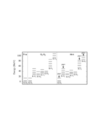
Figure 18: Energy spectra for ¹²C. Comparison between experimental values (left), results from a symplectic $8\hbar\omega$ calculation (center) and a PDS calculation (right). K=$0_{1}$ indicates the ground band in all three parts of the figure. In addition, resonance bands dominated by 2$\hbar\omega$ excitations (K=$2_{1},0_{2},1_{1},0_{3}$), 4$\hbar\omega$ excitations (K=$4_{1}$), and 6$\hbar\omega$ excitations (K=$6_{1}$) are shown for the Sp(6,R) and PDS calculations. Additional mixed resonance bands (not shown), dominated by 4$\hbar\omega$ and 6$\hbar\omega$ excitations, exist for this nucleus. The angular momenta of the positive parity states in the rotational bands are $L$=0,2,4,$\ldots$ for K=0 and $L$=K,K+1,K+2, $\ldots$ otherwise. Bands which consist of pure-SU(3) eigenstates of the PDS Hamiltonian (196) are indicated. Adapted from [115].

Table 14: B(E2) values (in Weisskopf units) for ground band transitions in ¹²C. Compared are several symplectic calculations, PDS results, and experimental data. Q denotes the static quadrupole moment of the $L^{\pi}=2^{+}_{1}$ state in units of $eb$. PDS results are rescaled by an effective charge e^∗=1.33 and the symplectic calculations employ bare charges. Adapted from [115].

Transition	Model B(E2) [W.u.]					B(E2) [W.u.]
$J_{i}\rightarrow J_{f}$	$2\hbar\omega$	$4\hbar\omega$	$6\hbar\omega$	$8\hbar\omega$	PDS	Exp
2 $\rightarrow$ 0	4.65	4.65	4.65	4.65	4.65	4.65 $\pm$ 0.26
4 $\rightarrow$ 2	4.35	4.27	4.24	4.23	4.28	n/a
$Q$ [eb]	0.059	0.060	0.060	0.060	0.058	0.06$\pm$ 0.03

Figure 19: Energy spectra for ²⁰Ne. Experimental ground band (K=$0_{1}$) energies (left), compared to theoretical results for both the ground band and 2$\hbar\omega$ resonances (K=$0_{2},1_{1},2_{1},0_{3}$) for a symplectic $8\hbar\omega$ calculation (center) and a PDS calculation (right). Rotational bands which consist of pure eigenstates of the PDS Hamiltonian are indicated. Adapted from [115].

²⁰Ne                                                         ¹²C

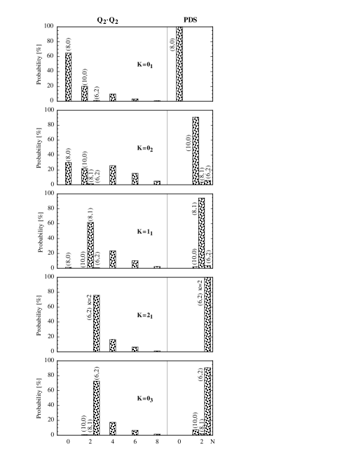
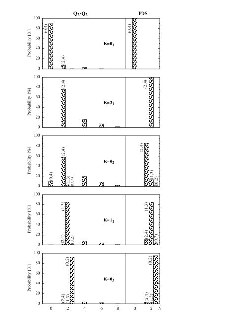
Figure 20: Decompositions for calculated $2^{+}$ states of ²⁰Ne (left) and ¹²C (right). Individual contributions from the relevant SU(3) irreps at the 0$\hbar\omega$ and 2$\hbar\omega$ levels are shown for both a symplectic $8\hbar\omega$ calculation (denoted $Q_{2}\cdot Q_{2}$) and a PDS calculation. In addition, the total strengths contributed by the $N\hbar\omega$ excitations for $N>2$ are given for the symplectic case. Adapted from [115].

Table 15: B(E2) values (in Weisskopf units) for ground band transitions in ²⁰Ne. Compared are several symplectic calculations, PDS results, and experimental data. The static quadrupole moment of the $2^{+}_{1}$ state is given in the last row. PDS results are rescaled by an effective charge e^∗=1.95 and the symplectic calculations employ bare charges. Adapted from [115].

Transition	Model B(E2) [W.u.]					B(E2) [W.u.]
$J_{i}\rightarrow J_{f}$	$2\hbar\omega$	$4\hbar\omega$	$6\hbar\omega$	$8\hbar\omega$	PDS	Exp
2 $\rightarrow$ 0	14.0	18.7	19.1	19.3	20.3	20.3 $\pm$ 1.0
4 $\rightarrow$ 2	18.4	24.5	24.6	24.5	25.7	22.0 $\pm$ 2.0
6 $\rightarrow$ 4	17.1	22.3	21.5	20.9	21.8	20.0 $\pm$ 3.0
8 $\rightarrow$ 6	12.4	15.2	13.3	12.4	12.9	9.0 $\pm$ 1.3
$Q$ [eb]	-0.14	-0.16	-0.16	-0.16	-0.17	-0.23 $\pm$ 0.03

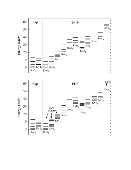
Figure 21: Energy spectra for ²⁴Mg. Energies from a PDS calculation (bottom) are compared to symplectic results (top). Both 0$\hbar\omega$ dominated bands (K=$0_{1},2_{1},4_{1}$) and some 2$\hbar\omega$ resonance bands (K=$0_{2},0_{3},0_{4},2_{2},2_{3},4_{2},4_{3},6_{1}$) are shown. The K=$0_{1},2_{1},4_{1}$ ($6_{1}$) states are pure (approximately pure) in the PDS scheme. Experimental energies of the ground and $\gamma$ bands are shown on the left. Adapted from [115].

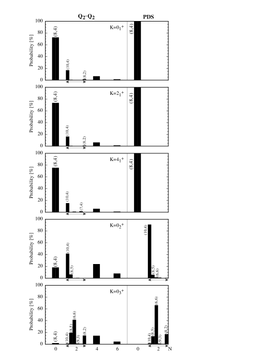
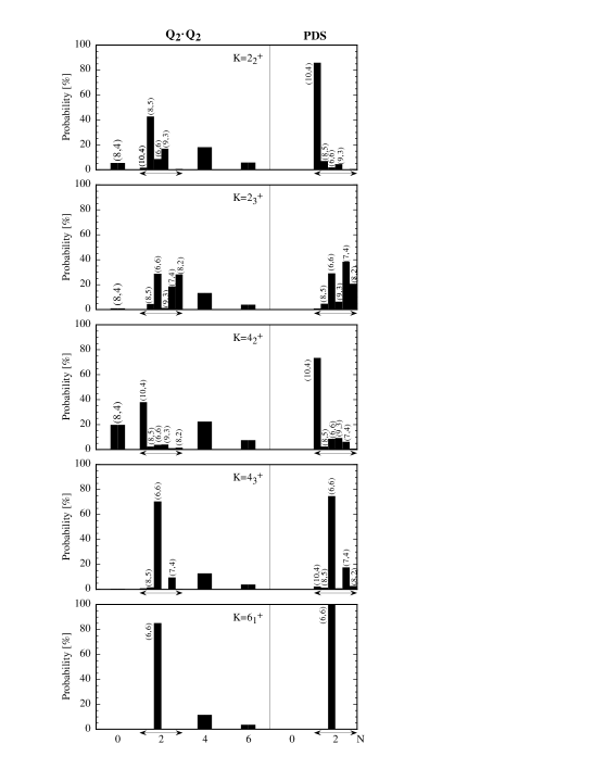
Figure 22: Decompositions for calculated $L^{\pi}=6^{+}$ states of ²⁴Mg. Eigenstates resulting from the symplectic 6$\hbar\omega$ calculation (denoted $Q_{2}\cdot Q_{2}$) are decomposed into their 0$\hbar\omega$, 2$\hbar\omega$, 4$\hbar\omega$, and 6$\hbar\omega$ components. At the 0$\hbar\omega$ and 2$\hbar\omega$ levels, contributions from the individual SU(3) irreps are shown, for higher excitations ($N>2$) only the summed strengths are given. Eigenstates of the PDS Hamiltonian belong entirely to one $N\hbar\omega$ level of excitation, here 0$\hbar\omega$ or 2$\hbar\omega$. Contributions from the individual SU(3) irreps at these levels are shown. Members of the K=$0_{1},2_{1},4_{1}$ bands are pure in the PDS scheme, and K=$6_{1}$ states are very nearly ($>99\%$) pure. Adapted from [115].

• $\lambda_{\sigma}>\mu_{\sigma}$: the pure states belong to $(\lambda,\mu)=(\lambda_{\sigma}-N,\mu_{\sigma}+N)$ at the $N\hbar\omega$ level and have $L=\mu_{\sigma}+N,\mu_{\sigma}+N+1,\ldots,\lambda_{\sigma}-N+1$ with $N=2,4,\ldots$ subject to $2N\leq(\lambda_{\sigma}-\mu_{\sigma}+1)$.

• $\lambda_{\sigma}\leq\mu_{\sigma}$: the special states belong to $(\lambda,\mu)=(\lambda_{\sigma}+N,\mu_{\sigma})$ at the $N\hbar\omega$ level and have $L=\lambda_{\sigma}+N,\lambda_{\sigma}+N+1,\ldots,\lambda_{\sigma}+N+\mu_{\sigma}$ with $N=2,4,\ldots$.

To prove the claim, it is sufficient to show that $\hat{B}_{0}$ annihilates the states in question

$$\hat{B}_{0}\,|\phi_{LM}(N)\rangle = 0~{}.$$ (193)

For $N=0$ this follows immediately from the fact that the $0\hbar\omega$ starting configuration is a Sp(6,R) lowest weight which, by definition, is annihilated by the lowering operators of the Sp(6,R) algebra. The latter include the generators $\hat{B}^{(02)}_{lm}$. For $N>0$, let $\{\sigma_{1},\sigma_{2},\sigma_{3}\}$ be the quanta distribution for a 0$\hbar\omega$ state with $\lambda_{\sigma}>\mu_{\sigma}$. Adding $N$ quanta to the 2-direction yields a $N\hbar\omega$ state with quanta distribution $\{\sigma_{1},\sigma_{2}+N,\sigma_{3}\}$, that is, $(\lambda,\mu)=(\lambda_{\sigma}-N,\mu_{\sigma}+N)$. Acting with the rotational invariant $\hat{B}_{0}$ on such a state does not affect the angular momentum, but removes two quanta from the 2-direction, giving a $(N-2)\hbar\omega$ state with $(\lambda^{\prime},\mu^{\prime})=(\lambda_{\sigma}-N+2,\mu_{\sigma}+N-2)$. (The symplectic generator $\hat{B}_{0}$ cannot remove quanta from the other two directions of this particular state, since this would yield a state belonging to a different symplectic irrep.) Comparing the number of $L$ occurrences in $(\lambda,\mu)$ and $(\lambda^{\prime},\mu^{\prime})$, one finds that as long as $\lambda_{\sigma}-N+1\geq\mu_{\sigma}+N$, $\Delta_{L}(N)\equiv\kappa_{L}^{max}(\lambda,\mu)-\kappa_{L}^{max}(\lambda^{\prime},\mu^{\prime})=1$ for $L=\mu_{\sigma}+N,\mu_{\sigma}+N+1,\ldots,\lambda_{\sigma}-N+1$, and $\Delta_{L}(N)=0$ otherwise. Therefore, when $\Delta_{L}(N)$=1, a linear combination $|\phi_{L}(N)\rangle=\sum_{\kappa}c_{\kappa}|N\hbar\omega(\lambda_{\sigma}-N,\mu_{\sigma}+N)\kappa LM\rangle$ exists such that $\hat{B}_{0}|\phi_{L}(N)\rangle=0$, and thus the claim for family (a) holds. The proof for family (b) can be carried out analogously. Here the special irrep $(\lambda,\mu)=(\lambda_{\sigma}+N,\mu_{\sigma})$ is obtained by adding $N$ quanta to the 1-direction of the starting configuration. In this case there is no restriction on $N$, hence family (b) is infinite.

The special states have well defined symmetry with respect to the chain (191) and the condition of Eq. (193) ensures that they are solvable eigenstates of $\hat{H}(\beta_{0},\beta_{2})$ (192) with eigenvalues $E(N=0)=0$ for the 0$\hbar\omega$ level, and

$$E(N) = \beta_{2}\frac{N}{3}(N_{\sigma}-\lambda_{\sigma}+\mu_{\sigma}-6+\frac{3}{2}N)\;\;\;\;(\lambda_{\sigma}>\mu_{\sigma})$$ (194a)

$$E(N) = \beta_{2}\frac{N}{3}(N_{\sigma}+2\lambda_{\sigma}+\mu_{\sigma}-3+\frac{3}{2}N)\;\;\;\;(\lambda_{\sigma}\leq\mu_{\sigma})$$ (194b)

for $N>0$. All 0$\hbar\omega$ states are unmixed and span the entire $(\lambda_{\sigma},\mu_{\sigma})$ irrep. In contrast, for the excited levels ($N>0$), the pure states span only part of the corresponding SU(3) irreps. There are other states at each excited level which do not preserve the SU(3) symmetry and therefore contain a mixture of SU(3) irreps. The partial SU(3) symmetry of $\hat{H}(\beta_{0},\beta_{2})$ is converted into SU(3)-PDS of type I by adding to it O(3) rotation terms which lead to L(L+1)-type splitting but do not affect the wave functions. The solvable states then form rotational bands and since condition (193) determines their wave functions, one can obtain analytic expressions for the E2 rates between them [115].

The Hamiltonian of Eq. (192), with SU(3) partial symmetry, has a close relationship to the collective quadrupole- quadrupole interaction,

$$Q_{2}\cdot Q_{2}=3(\hat{C}_{2}+\hat{A}_{2}+\hat{B}_{2})\cdot(\hat{C}_{2}+\hat{A}_{2}+\hat{B}_{2})$$ (195)

$$=\hat{H}(\beta_{0}=12,\beta_{2}=18)+const-3\hat{L}^{2}+\{\mbox{terms coupling different h.o. shells}\}~{}.\qquad\;\;\,$$

Here $const=6\hat{C}_{{\rm Sp(6)}}-2\hat{H}_{0}^{2}+34\hat{H}_{0}$ is fixed for a given symplectic irrep $N_{\sigma}(\lambda_{\sigma},\mu_{\sigma})$ and $N\hbar\omega$ excitation. Although $\hat{H}(\beta_{0},\beta_{2})$ does not couple different harmonic oscillator shells, it breaks the SU(3)-symmetry and, due to the above relation, exhibits in-shell behavior similar to that of $Q_{2}\cdot Q_{2}$. To study this connection further, and to illustrate that the PDS Hamiltonians of Eq. (192) are physically relevant, the formalism was applied to oblate prolate and triaxially deformed nuclei, by comparing the properties of the following SU(3)-PDS Hamiltonian

$$\hat{H}_{PDS} = h(N)+\xi\hat{H}(\beta_{0}=12,\beta_{2}=18)+\gamma_{2}\hat{L}^{2}+\gamma_{4}\hat{L}^{4}$$ (196)

to those of the symplectic Hamiltonian

$$\hat{H}_{{\rm Sp(6)}} = \hat{H}_{0}-\eta Q_{2}\cdot Q_{2}+d_{2}\hat{L}^{2}+d_{4}\hat{L}^{4}\;.$$ (197)

Here the function $h(N)$, which contains the harmonic oscillator term $\hat{H}_{0}$, is simply a constant for a given $N\hbar\omega$ excitation. Details of the calculations can be found in [115].

The leading Sp(6,R) irrep for the oblate nucleus ¹²C is $N_{\sigma}(\lambda_{\sigma},\mu_{\sigma})$ $=24.5(0,4)$. In this case, $\hat{H}_{PDS}$ (196) has the pure-SU(3) states of family (b) as solvable eigenstates. In particular, all 0$\hbar\omega$ states are pure $(\lambda_{\sigma},\mu_{\sigma})=(0,4)$ states, and at 2$\hbar\omega$ a rotational band with good SU(3) symmetry $(\lambda,\mu)=(2,4)$ and $L=2,3,4,5,6$ exists. Similarly, at 4$\hbar\omega$ there are pure-SU(3) bands with $(\lambda,\mu)=(4,4)$ and $L=4,5,6,7,8$, at 6$\hbar\omega$ with $(\lambda,\mu)=(6,4)$ and $L=6,7,8,9,10$, etc. On the other hand, the leading Sp(6,R) irrep for the prolate nucleus ²⁰Ne is $N_{\sigma}(\lambda_{\sigma},\mu_{\sigma})$ $=48.5(8,0)$. In this case, the solvable pure-SU(3) eigenstates of $\hat{H}_{PDS}$ are those of family (a). They form a K=$0_{1}$ $L=0,2,4,6,8$ rotational band with $(\lambda,\mu)=$ (8,0) at 0$\hbar\omega$, a K=$2_{1}$ $L=2,3,4,5,6,7$ band with $(\lambda,\mu)=$ (6,2) at 2$\hbar\omega$, and a K=$4_{1}$ $L=4,5$ ‘band’ with $(\lambda,\mu)=$ (4,4) at 4$\hbar\omega$. There are no other pure PDS states at higher levels of excitation. As shown in Fig. 18 and Table 14 for ¹²C, and in Fig. 19 and Table 15 for ²⁰Ne, the resulting energies and transition rates in the PDS and symplectic approaches are similar and converge to values which agree with the data. The PDS calculations of B(E2) values, however, require an effective charge. A better measure for the level of agreement between the PDS and symplectic results is given by a comparison of the eigenstates. From Fig. 20 we observe that, although $\hat{H}_{{\rm Sp(6)}}$ (197) [$\hat{H}_{PDS}$ (196)] does (does not) mix different major oscillator shells, the $N\hbar\omega$ level to which a particular PDS band belongs is also dominant in the corresponding symplectic band. Furthermore, within this dominant excitation, eigenstates of $\hat{H}_{{\rm Sp(6)}}$ and $\hat{H}_{PDS}$ have very similar SU(3) structure, that is, the relative strengths of the various SU(3) irreps in the symplectic states are approximately reproduced in the PDS case. This holds for the ground and excited bands in both nuclei, with the exception of the K=$0_{2}$ resonance band in ²⁰Ne, where significant differences appear in the structure of the wave functions. Thus the SU(3)-PDS Hamiltonian captures much of the physics of the $Q_{2}\cdot Q_{2}$ interaction.

Calculations were also performed [115] for the triaxially-deformed nucleus, ²⁴Mg, whose leading Sp(6,R) irrep is $N_{\sigma}(\lambda_{\sigma},\mu_{\sigma})$ $=62.5(8,4)$. Since now both $\lambda_{\sigma}\neq 0$ and $\mu_{\sigma}\neq 0$, the symplectic Hilbert space has a very rich structure. In this case, the solvable pure-SU(3) states are those of family (a) and include three rotational K=0,2,4, bands at 0$\hbar\omega$ with $(\lambda,\mu)=(8,4)$, and at 2$\hbar\omega$ a (short) rotational K=6 band with $L$=6,7, which belongs to the irrep $(\lambda,\mu)=(6,6)$. Figure 21 compares the experimental spectrum of ²⁴Mg with energies obtained with 6$\hbar\omega$ symplectic and PDS calculations. Both the PDS and symplectic Hamiltonians were supplemented with small cubic and quartic SU(3)-conserving interactions to account for $K$-band splitting. These extra terms break the partial symmetry slightly ($<1\%$) in the $K=6_{1}$ band, as can be inferred from the eigenstate decompositions plotted in Fig. 22. As in the previous examples, the eigenstates of the PDS and symplectic Hamiltonians are found to have very similar structures. The structural differences that do exist are reflected in the very sensitive interband transition rates [115].

The boson Hamiltonian, $\hat{H}(h_{0},h_{2})$ of Eq. (43), and the fermion Hamiltonian, $\hat{H}(\beta_{0},\beta_{2})$ of Eq. (192), have several features in common. Both display partial SU(3) symmetry, they are constructed to be rotationally invariant functions of $(\lambda,\mu)=(2,0)$ and $(\lambda,\mu)=(0,2)$ SU(3) tensor operators, and both contain components with $(\lambda,\mu)=(0,0)$ and $(2,2)$. Both Hamiltonian have solvable pure-SU(3) eigenstates, which can be organized into rotational bands. The ground bands are pure in both cases, and higher-energy pure bands coexist with mixed-symmetry states. There are, however, several significant differences between the bosonic and fermionic PDS Hamiltonians. For example, the ground band of the bosonic Hamiltonian $\hat{H}(h_{0},h_{2})$, Eq. (43), is characterized by $(\lambda,\mu)=(2N,0)$, i.e., it describes an axially-symmetric prolate nucleus. As mentioned at the end of Subsection 2.2, it is also possible to find an IBM Hamiltonian with partial SU(3) symmetry for an oblate nucleus. It can be shown that these two cases exhaust all possibilities for partial SU(3) symmetry with a two-body Hamiltonian in the IBM with one type of monopole and quadrupole bosons. In contrast, the fermionic Hamiltonian $\hat{H}(\beta_{0},\beta_{2})$ (192) can accommodate ground bands of prolate [$(\lambda_{\sigma},0)$], oblate [$(0,\mu_{\sigma})$], and triaxial [$(\lambda_{\sigma},\mu_{\sigma})$ with $\lambda_{\sigma}\neq 0$, $\mu_{\sigma}\neq 0$] shapes. Another difference lies in the physical interpretation of the excited solvable bands. While these bands represent $\gamma^{k}$ excitations in the IBM, they correspond to giant monopole and quadrupole resonances in the fermion case. Furthermore, whereas the pure eigenstates of the IBM Hamiltonian $\hat{H}(h_{0},h_{2})$ can be generated by angular momentum projection from intrinsic states (46), a similar straightforward construction process for the special eigenstates of the symplectic Hamiltonian $\hat{H}(\beta_{0},\beta_{2})$ has not been identified yet. The situation seems to be more complicated in the fermion case, which is also reflected in the fact that $\hat{H}(\beta_{0},\beta_{2})$ has two possible families of pure eigenstates, one finite, the other infinite. The association of the special states to one or the other family depends on the 0$\hbar\omega$ symplectic starting configuration. Thus, in spite of similar algebraic structures, the bosonic and fermionic PDS Hamiltonians involve different mechanisms for generating the partial symmetries in question.

10.2 PDS and seniority

The notions of pairing and seniority for $n$ identical nucleons occupying a single $j$ shell, are conveniently encoded in the quasi-spin formalism [3]. The latter is based on an ${\rm SU}_{S}(2)$ algebra whose generators are

$$\hat{S}^{+}_{j}=\sqrt{\frac{\Omega}{2}}\,(a^{{\dagger}}_{j}\,a^{{\dagger}}_{j})^{(0)}_{0}\;\;\;,\;\;\;\hat{S}^{-}_{j}=(\hat{S}^{+}_{j})^{{\dagger}}\;\;\;,\;\;\;\hat{S}^{0}_{j}=\frac{1}{2}(\hat{n}-\Omega)~{}.$$ (198)

Here $\hat{S}^{+}_{j}$ creates a pair of fermions with angular momentum $J=0$, $\hat{n}=\sum_{m}a^{{\dagger}}_{jm}a_{jm}$ is the number-operator and $\Omega=(2j+1)/2$. The basic quasi-spin doublet is $(a^{{\dagger}}_{jm},\,-\tilde{a}_{jm})$, with $\tilde{a}_{jm}=(-1)^{j+m}a_{j,-m}$. The seniority quantum number, $v$, refers to the number of nucleons which are not in zero-coupled $J=0$ pairs. The ${\rm SU}_{S}(2)$ quantum numbers, $(S,S_{0})$ are related to $n$ and $v$ by

$$S=(\Omega-v)/2\;\;\;,\;\;\;S_{0}=(n-\Omega)/2~{}.$$ (199)

The operator $\hat{S}^{-}_{j}$ annihilates states with $(S,S_{0}=-S)$ corresponding to states in the $j^{v}$ configuration with seniority $v$ and $n=v$.

The relevant chain of nested algebras for $n$ fermions in a single $j$ shell is [126, 127]

$$\begin{array}[]{ccccc}{\rm U(2j+1)}&\supset&{\rm Sp(2j+1)}&\supset&{\rm SU_{J}(2)}\\ \downarrow&&\downarrow&&\downarrow\\ \left[1^{n}\right]&&v&\rho&J\end{array}~{},$$ (203)

where $\rho$ is a multiplicity index. The generators of the indicated algebras are

$${\rm U(2j+1)}=\{\hat{T}^{(L)}_{m}\}\;\;,\;\;{\rm Sp(2j+1)}=\{\hat{T}^{(L)}_{m}\;L\,{\rm odd}\}~{},$$

$${\rm SU_{J}(2)}=\{\hat{J}_{m}=c_{j}\,\hat{T}^{(1)}_{m}\}\;\;,\;\;c_{j}=\sqrt{j(j+1)(2j+1)/3}~{},\qquad$$ (204)

where

$$\hat{T}^{(L)}_{m}=\left(a^{{\dagger}}_{j}\,\tilde{a}_{j}\right)^{(L)}_{m}\qquad L=0,1,2,\ldots,2j~{}.$$ (205)

The unitary symplectic algebra, Sp(2j+1), and quasi-spin algebra, ${\rm SU}_{S}(2)$, commute. The duality relationship between their respective irreps, $v$ and $S$, is given in Eq. (199) and their quadratic Casimir operators are related by $\hat{C}_{2}[{\rm Sp(2j+1)}]=\Omega(\Omega+2)-4\mbox{\boldmath$\hat{S}^{2}$}$. The dynamical symmetry Hamiltonian associated with the chain (203) is given by

$$\hat{H}_{DS} = \beta\,\hat{n}+\alpha\,\hat{n}(\hat{n}-1)+a\,\hat{C}_{2}[{\rm Sp(2j+1)}]+b\,\hat{C}_{2}[{\rm SU_{J}(2)}]~{},$$ (206a)

$$E_{DS} = \beta\,n+\alpha\,n(n-1)+a\,v(2\Omega+2-v)+b\,J(J+1)~{},$$ (206b)

and $E_{DS}$ are the corresponding eigenvalues.

The $\hat{T}^{(L)}_{m}$ operators of Eq. (205), with $L$ odd, are quasi-spin scalars. Accordingly, the most general number-conserving rotational invariant Hamiltonian with seniority-conserving one- and two-body interactions, acting in a single-$j$ shell, can be transcribed in the form [17]

$$\hat{H} = \beta\,\hat{n}+\alpha\,\hat{n}(\hat{n}-1)+\sum_{L\,{\rm odd}}\lambda_{L}\,\hat{T}^{(L)}\cdot\hat{T}^{(L)}$$ (207a)

$$E_{n,v,\rho,J} = \beta\,n+\alpha\,n(n-1)+Z_{v,\rho,J}~{}.$$ (207b)

For the special choice, $\lambda_{L}=2a+b\,c_{j}^{2}\,\delta_{L,1}$, the above Hamiltonian reduces to the dynamical symmetry Hamiltonian of Eq. (206a). In general, eigenstates of $\hat{H}$ (207) are basis states, $|n,v,\rho,JM\rangle$, of the chain (203) with eigenvalues $E_{n,v,\rho,J}$ and wave functions of the form

$$|n,v,\rho,JM\rangle\propto\left(\hat{S}_{j}^{+}\right)^{(n-v)/2}|n=v,j,v,\rho,JM\rangle~{}.$$ (208)

Since the last term in Eq. (207a) is a quasi-spin scalar, its eigenvalues, $Z_{v,\rho,J}$, are independent of $n$. Consequently, for a given $n$, energy differences $E_{n,j,v,\rho,J}-E_{n,j,v^{\prime},\rho^{\prime},J^{\prime}}$, are independent of $n$. Conservation of seniority does not, however, imply solvability. In general, eigenstates and eigenvalues of $\hat{H}$, Eq. (207), must be obtained from a numerical calculation. Nevertheless, it has been shown that some multiplicity-free eigenstates of $\hat{H}$, i.e., with unique $n,v,J$ assignments, are completely solvable and closed algebraic expressions for their energies have been derived [116, 117]. These include states with $(v=2,J)$, $(v,J_{max})$ and $(v,J_{max}-2)$, where $J_{max}=v(2j+1-v)/2$. As an example, for $n$ even, the ground state of $\hat{H}$ (207a), with $v=J=0$, is analytically solvable with energy

$$E_{n,j,v=0,J=0} = \beta\,n+\alpha\,n(n-1)~{}.$$ (209)

The above expression is identical to the ground-state energy of the dynamical symmetry Hamiltonian, Eq. (206). Since all eigenstates carry the seniority quantum number $v$, the Hamiltonian $\hat{H}$ of Eq. (207) exhibits PDS of type II with an added feature that some multiplicity-free states are analytically solvable.

As is well known [17], seniority remains a good quantum number for any two-body interaction acting within a $j$ shell when $j\leq 7/2$, but it need not be conserved for $j\geq 9/2$. Recently, it has been shown that it is possible to construct interactions that in general do not conserve seniority but which have some solvable eigenstates with good seniority [118, 120]. Specifically, for $j=9/2,\,n=4$, there are two independent states ($\rho=1,2$) with seniority $v=4$ and $J=4,\,6$. For each such $J$ value, there exists one particular combination, which is completely solvable with good seniority, $v=4$, for any two-body interaction in the $j=9/2$ shell. The energies of the solvable states are given by [120]

$$E[(9/2)^{4},v=4,J=4] = \frac{68}{33}\,\nu_{2}+\nu_{4}+\frac{13}{15}\,\nu_{6}+\frac{114}{55}\,\nu_{8}~{},$$ (210a)

$$E[(9/2)^{4},v=4,J=6] = \frac{19}{11}\,\nu_{2}+\frac{12}{13}\,\nu_{4}+\nu_{6}+\frac{336}{143}\,\nu_{8}~{},$$ (210b)

where $\nu_{\lambda}\equiv\langle(9/2)^{2};\lambda|\hat{V}|(9/2)^{2};\lambda\rangle$ are the matrix elements of an arbitrary rotational-invariant two-body interaction, $\hat{V}$. The indicated states retain their structure and are completely solvable, independent of whether the interaction conserves seniority or not. It follows that the most general one- and two-body rotational-invariant Hamiltonian in the $j=9/2$ shell, exhibits PDS of type I. The E2 matrix element between the two solvable states is interaction-independent, and the corresponding B(E2) value is given by [120]

$$B(E2;(9/2)^{4},v=4,J=6\to(9/2)^{4},v=4,J=4)=$$

$$\qquad\qquad\qquad\qquad\qquad\qquad\frac{209475}{176468}\,B(E2;(9/2)^{2},J=2\to(9/2)^{2},J=0)~{}.$$ (211)

This again defines a parameter-independent relation between a property of the two- and four-particle system. Some properties of these solvable states can be attributed to properties of certain coefficients of fractional parentage [119, 120, 121, 122]. It has been suggested that this partial seniority conservation may shed some new light on the existence of isomers in nuclei with valence neutrons or protons predominantly confined to the $g_{9/2}$ or $h_{9/2}$ shell [120].

In most medium-mass and heavy nuclei, the valence nucleons are distributed over several non-degenerate $j$ orbits in a major shell. This situation can be treated within the generalized seniority scheme [128], based on more general pair-operators with $J=0,2$

$$\hat{S}^{{\dagger}} = \sum_{j}\alpha_{j}\,(a^{{\dagger}}_{j}\,a^{{\dagger}}_{j})^{(0)}_{0}~{},$$ (212a)

$$D^{{\dagger}}_{\mu} = \sum_{j,j^{\prime}}\beta_{jj^{\prime}}\,(a^{{\dagger}}_{j}\,a^{{\dagger}}_{j^{\prime}})^{(2)}_{\mu}~{}.$$ (212b)

The generalized seniority conditions [128, 129, 130] are

$$\hat{H}|0\rangle = 0~{},$$ (213a)

$$\left[\,\hat{H}\,,\,S^{{\dagger}}\,\right]|0\rangle = V_{0}\,S^{{\dagger}}|0\rangle\;\;,\;\;\left[\left[\,\hat{H}\,,\,S^{{\dagger}}\,\right]\,,\,S^{{\dagger}}\,\right]=\Delta\,(S^{{\dagger}})^{2}~{},$$ (213b)

$$\left[\,\hat{H}\,,\,D^{{\dagger}}_{\mu}\,\right]|0\rangle = V_{2}\,D^{{\dagger}}_{\mu}|0\rangle\;\;,\;\;\left[\left[\,\hat{H}\,,\,S^{{\dagger}}\,\right]\,,\,D^{{\dagger}}_{\mu}\,\right]=\Delta\,S^{{\dagger}}D^{{\dagger}}_{\mu}~{},$$ (213c)

where $|0\rangle$ is the doubly-magic core state. These relations imply that the Hamiltonian has a solvable ground state with $J=0$ and generalized seniority $v_{g}=0$

$$|n=2N,v_{g}=0,J=0\rangle \propto \left(S^{{\dagger}}\right)^{N}|0\rangle~{},$$ (214a)

$$E_{N,v_{g}=0,J=0} = N\,V_{0}+\frac{1}{2}N(N-1)\,\Delta~{},$$ (214b)

and a solvable excited state with $J=2$ and generalized seniority $v_{g}=2$

$$|n=2N,v_{g}=2,J=2\rangle \propto \left(S^{{\dagger}}\right)^{N-1}D^{{\dagger}}_{\mu}|0\rangle~{},$$ (215a)

$$E_{N,v_{g}=2,J=2} = E_{N,v_{g}=0,J=0}+V_{2}-V_{0}~{}.$$ (215b)

From the point of view of symmetry, the monopole pair-operators $S^{{\dagger}},\,S$, and $\left[S^{{\dagger}}\,,\,S\right]/2$, of Eq. (212a), with unequal $\alpha_{j}$, do not form an SU(2) algebra. Nevertheless, an Hamiltonian $\hat{H}$ satisfying relations (213) has selected solvable states, i.e., it is partially solvable. It should be noted that the energy and wave function of the $v_{g}=0$ ground state (214) have the same form as in the single-$j$ dynamical symmetry expressions, Eqs. (208)-(209) and, by construction, both spectra exhibit linear two-nucleon separation energies and constant $2^{+}$-$0^{+}$ spacings. Furthermore, the Sp(2j+1) generators (204), $\hat{T}^{(L)}_{m}$ with L odd and any $j$, annihilate the state of Eq. (214). Therefore, the $v_{g}=0$ ground state is invariant under $\prod_{j}\otimes{\rm Sp(2j+1)}$, even though the latter is not a symmetry of the Hamiltonian.

11 Concluding Remarks

The notion of partial dynamical symmetry (PDS) extends and complements the fundamental concepts of exact and dynamical symmetries. It addresses situations in which a prescribed symmetry is neither exact nor completely broken. When found, such intermediate symmetry structure can provide analytic solutions and quantum numbers for a portion of the spectra, thus offering considerable insight into complex dynamics. In other circumstances a PDS can serve as a convenient starting point for further improvements.

As discussed in the present review, PDSs of various types have concrete applications to nuclear and molecular spectroscopy. Their empirical manifestations illustrate their ability to serve as a practical tool for calculation of observables in realistic systems. Hamiltonians with partial symmetries are not completely integrable nor fully chaotic. As such, they are relevant to the study of mixed systems with coexisting regularity and chaos, which are the most generic. Quantum phase transitions are driven by competing symmetries in the Hamiltonian. They provide a natural arena for PDSs, which incorporate such incompatible symmetries, and manage to survive at the critical points, in spite of the strong mixing.

PDSs appear to be a common feature in algebraic descriptions of dynamical systems. They are not restricted to a specific model but can be applied to any quantal systems of interacting particles, bosons and fermions. The existence of PDS is closely related to the order of the interaction among the particles. The partial symmetry in question can be continuous (Lie-type), or discrete (point-group) and the associated dynamical algebra can involve a single or coupled algebraic structure. The examples of partial dynamical symmetries surveyed in the present review, involved purely bosonic or purely fermionic algebras. It is clearly desirable to extend the PDS notion to mixed systems of bosons and fermions, and explore the possible role of partial Bose-Fermi symmetries and partial supersymmetries.

On phenomenological grounds, having at hand concrete algorithms for identifying and constructing Hamiltonians with PDS, is a valuable asset. It provides selection criteria for the a priori huge number of possible symmetry-breaking terms, accompanied by a rapid proliferation of free-parameters. This is particularly important in complicated environments when many degrees of freedom take part in the dynamics and upon inclusion of higher-order terms in the Hamiltonian. Futhermore, Hamiltonians with PDS break the dynamical symmetry (DS) but retain selected solvable eigenstates with good symmetry. The advantage of using interactions with a PDS is that they can be introduced, in a controlled manner, without destroying results previously obtained with a DS for a segment of the spectrum. These virtues greatly enhance the scope of applications of algebraic modeling of quantum many-body systems.

On a more fundamental level, it is important to recall that dynamical systems often display simple patterns amidst a complicated environment. A representative example is the occurrence of both collective and quasi-particle type of states in the same nucleus. It is natural to associate the “simple” states with a symmetry that protects their purity and special character. This symmetry, however, is shared by only a subset of states, and is broken in the remaining eigenstates of the same Hamiltonian. It thus appears that realistic quantum many-body Hamiltonians can accommodate simultaneously eigenstates with different symmetry character. These are precisely the defining ingredients of a partial symmetry. In this context, PDS can offer a possible clue to the deep question of how simple features emerge from complicated dynamics.

Underlying the PDS notion, is the recognition that it is possible for a non-invariant Hamiltonian to have selected eigenstates with good symmetry and good quantum numbers. In such a case, the symmetry in question is preserved in some states but is broken in the Hamiltonian (an opposite situation to that encountered in a spontaneously-broken symmetry). The PDS concept is, therefore, relevant to situations where selected states fulfill the predictions of a symmetry, which is otherwise known to be broken. Familiar examples of such a scenario include flavor symmetry in hadrons and chiral symmetry in nuclei. PDS may thus shed a new light on the related question of why, occasionally, symmetries seem to be obeyed beyond their domain of validity.

The realistic attributes and fundamental aspects of partial symmetries, as portrayed in the present review, illuminate their potential useful role in dynamical systems and motivate their ongoing and future in-depth study. Much has been learnt but much more awaits to be explored and understood.

Appendix

Table 16: Generators and Casimir operators, $\hat{C}_{G}$, of algebras $G$ in the IBM. Here $\hat{n}_{d}=\sqrt{5}\,U^{(0)}$, $L^{(1)}=\sqrt{10}\,U^{(1)}$, $Q^{(2)}=\Pi^{(2)}-{\textstyle\frac{\sqrt{7}}{2}}\,U^{(2)}$, $\bar{Q}^{(2)}=\Pi^{(2)}+{\textstyle\frac{\sqrt{7}}{2}}\,U^{(2)}$. The operators $U^{(L)},\,\Pi^{(2)},\,\bar{\Pi}^{(2)},\,\hat{n}_{s}$, are defined in Eq. (1).

Algebra	Generators	Irrep.	Casimir operator	Eigenvalues
O(3)	$U^{(1)}$	L	$L^{(1)}\cdot L^{(1)}$	L(L+1)
O(5)	$U^{(1)},U^{(3)}$	$\tau$	$2(U^{(1)}\cdot U^{(1)}+U^{(3)}\cdot U^{(3)})$	$\tau(\tau+3)$
O(6)	$U^{(1)},U^{(3)},\Pi^{(2)}$	$\sigma$	$\hat{C}_{{\rm O(5)}}+\Pi^{(2)}\cdot\Pi^{(2)}$	$\sigma(\sigma+4)$
$\overline{{\rm O(6)}}$	$U^{(1)},U^{(3)},\bar{\Pi}^{(2)}$	$\bar{\sigma}$	$\hat{C}_{{\rm O(5)}}+\bar{\Pi}^{(2)}\cdot\bar{\Pi}^{(2)}$	$\bar{\sigma}(\bar{\sigma}+4)$
SU(3)	$U^{(1)},Q^{(2)}$	$(\lambda,\mu)$	$2Q^{(2)}\cdot Q^{(2)}+{\textstyle\frac{3}{4}}L^{(1)}\cdot L^{(1)}$	$\lambda^{2}+(\lambda+\mu)(\mu+3)$
$\overline{{\rm SU(3)}}$	$U^{(1)},\bar{Q}^{(2)}$	$(\bar{\lambda},\bar{\mu})$	$2\bar{Q}^{(2)}\cdot\bar{Q}^{(2)}+{\textstyle\frac{3}{4}}L^{(1)}\cdot L^{(1)}$	$\bar{\lambda}^{2}+(\bar{\lambda}+\bar{\mu})(\bar{\mu}+3)$
U(5)	$U^{(L)}$ $L=0,\ldots,4$	$n_{d}$	$\hat{n}_{d},\,\hat{n}_{d}(\hat{n}_{d}+4)$	$n_{d},\,n_{d}(n_{d}+4)$
U(6)	$U^{(L)}$ $L=0,\ldots,4$	$N$	$\hat{N},\,\hat{N}(\hat{N}+5)$	$N,\,N(N+5)$
	$\Pi^{(2)},\,\bar{\Pi}^{(2)},\,\hat{n}_{s}$

The normal-order form of the most general IBM Hamiltonian with one- and two-body interactions is given by

$$\hat{H}_{IBM} = \epsilon_{s}\,s^{{\dagger}}s+\epsilon_{d}\,d^{{\dagger}}\cdot\tilde{d}+u_{0}\,(s^{{\dagger}})^{2}s^{2}+u_{2}\,s^{{\dagger}}d^{{\dagger}}\cdot\tilde{d}s+v_{0}\,\left[\,(s^{{\dagger}})^{2}\tilde{d}\cdot\tilde{d}+H.c.\,\right]$$ (216)

$$+v_{2}\,\left[\,s^{{\dagger}}d^{{\dagger}}\cdot(\tilde{d}\tilde{d})^{(2)}+H.c.\,\right]+\sum_{L=0,2,4}c_{L}\,(d^{{\dagger}}d^{{\dagger}})^{(L)}\cdot(\tilde{d}\tilde{d})^{(L)}~{}.$$

The corresponding multipole form, written in terms of the Casimir operators listed in Table 16, is given by

$$\hat{H}_{IBM} = \epsilon_{s}\,\hat{N}+u_{0}\,\hat{N}(\hat{N}-1)+(\epsilon_{d}-\epsilon_{s})\,\hat{n}_{d}-(2u_{0}-u_{2}+2v_{0})\,(\hat{N}-1)\hat{n}_{d}$$ (217)

$$+(u_{0}-u_{2}+2v_{0}+{\textstyle\frac{1}{2\sqrt{7}}}v_{2}+{\textstyle\frac{1}{5}}c_{0}+{\textstyle\frac{2}{7}}c_{2}+{\textstyle\frac{18}{35}}c_{4})\hat{n}_{d}(\hat{n}_{d}-1)$$

$$-(v_{0}+{\textstyle\frac{3}{2\sqrt{7}}}v_{2}+{\textstyle\frac{1}{5}}c_{0}-{\textstyle\frac{2}{7}}c_{2}+{\textstyle\frac{3}{35}}c_{4})\left[\,\hat{C}_{{\rm O(5)}}-4\hat{n}_{d}\,\right]-{\textstyle\frac{1}{2\sqrt{7}}}\,v_{2}\,\left[\,\hat{C}_{{\rm SU(3)}}-10\hat{N}\,\right]$$

$$+(v_{0}+{\textstyle\frac{1}{\sqrt{7}}}v_{2})\left[\,\hat{C}_{{\rm O(6)}}-5\hat{N}\,\right]+({\textstyle\frac{1}{2\sqrt{7}}}v_{2}+{\textstyle\frac{1}{7}}c_{4}-{\textstyle\frac{1}{7}}c_{2})\left[\,\hat{C}_{{\rm O(3)}}-6\hat{n}_{d}\,\right]~{}.$$

References

- [1] For a general review see Dynamical Groups and Spectrum Generating Algebras, Eds. A. Bohm, Y. Néeman and A.O. Barut, World Scientific, 1988.
- [2] E. Wigner, Phys. Rev. 51 (1937) 106.
- [3] A. Kerman, Ann. Phys. (N.Y.) 12 (1961) 300.
- [4] J. P. Elliott, Proc. Roy. Soc. Lond. A 245 (1958) 128; ibid. 245 (1958) 562.
- [5] D. J. Rowe, Rep. Prog. Phys. 48 (1985) 1419.
- [6] R.D. Ratna-Raju, K.T. Hecht, B.D. Chang and J.P. Draayer, Nucl. Phys. A 202 (1973) 433.
- [7] J.N. Ginocchio, Ann. Phys. (N.Y.) 126 (1980) 234.
- [8] F. Iachello and A. Arima, The Interacting Boson Model, Cambridge Univ. Press, Cambridge 1987.
- [9] F. Iachello and P. Van Isacker, The Interacting Boson-Fermion Model, Cambridge Univ. Press, Cambridge, 1991.
- [10] F. Iachello and R.D. Levine, Algebraic Theory of Molecules, Oxford Univ. Press, Oxford, 1994.
- [11] A. Frank and P. Van Isacker, Algebraic Methods in Molecular and Nuclear Physics, Wiley, New York, 1994.
- [12] R. Bijker, F. Iachello and A. Leviatan, Ann. Phys. (N.Y.) 236 (1994) 69; ibid. 284 (2000) 89.
- [13] F. Iachello, Lie Algebras and Applications, Springer-Verlag, Berlin 2006.
- [14] A. Arima and F. Iachello, Ann. Phys. (N.Y.) 99 (1976) 253.
- [15] A. Arima and F. Iachello, Ann. Phys. (N.Y.) 111 (1978) 201.
- [16] A. Arima and F. Iachello, Ann. Phys. (N.Y.) 123 (1979) 468.
- [17] I. Talmi, Simple Models of Complex Nuclei: The Shell Model and Interacting Boson Model, Harwood Academic Publishers, Chur, 1993.
- [18] A. Bohr and B. R. Mottelson, Nuclear Structure II, Benjamin, Reading, MA, 1975.
- [19] J.N. Ginocchio and M.W. Kirson, Phys. Rev. Lett. 44 (1980) 1744; ibid., Nucl. Phys. A 350 (1980) 31.
- [20] A. E. L. Dieperink, O. Scholten and F. Iachello, Phys. Rev. Lett. 44 (1980) 1747.
- [21] P. Van Isacker and J.Q. Chen, Phys. Rev. C 24 (1981) 684.
- [22] A. Leviatan and B. Shao, Phys. Lett. B 243 (1990) 313.
- [23] Y. Alhassid and A. Leviatan, J. Phys. A 25 (1992) L1265.
- [24] J.E. García-Ramos, A. Leviatan and P. Van Isacker, Phys. Rev. Lett. 102 (2009) 112502.
- [25] A. V. Turbiner, Sov. Phys.-JETP 67 (1988) 230; M.A. Schifman, Int. J. Mod. Phys. A 4 (1989) 2897.
- [26] M. Moshinsky and C. Quesne, Ann. Phys. (N.Y.) 148 (1983) 462; H. Ui and G. Takeda, Prog. Theor. Phys. 72 (1984) 266; M. Moshinsky and C. Quesne and G. Loyola, Ann. Phys. (N.Y.) 198 (1983) 103.
- [27] D.J. Rowe, Nucl. Phys. A 745 (2004) 47; P.S. Turner and D.J. Rowe, ibid. 756 (2005) 333; G. Rosensteel and D.J. Rowe, ibid. 759 (2005) 92.
- [28] J.L. Ping and J.Q. Chen, Ann. Phys. (N.Y.) 255 (1997) 75.
- [29] S. Szpikowski and A. Góźdź, Nucl. Phys. A 340 (1980) 76.
- [30] J.D. Vergados, Nucl. Phys. A 111 (1968) 681.
- [31] R.F. Casten and D.D. Warner, Rev. Mod. Phys. 60 (1988) 389.
- [32] D.D. Warner, R.F. Casten and W.F. Davidson, Phys. Rev. C 24 (1981) 1713.
- [33] D.D. Warner and R.F. Casten, Phys. Rev. C 28 (1983) 1798.
- [34] H.T. Chen and A. Arima, Phys. Rev. Lett. 51 (1983) 447.
- [35] A. Leviatan, Phys. Rev. Lett. 77 (1996) 818.
- [36] P. Van Isacker, Phys. Rev. C 27 (1983) 2447.
- [37] A. Leviatan and I. Sinai, Phys. Rev. C 60 (1999) 061301.
- [38] For a review see, P.E. Garrett, J. Phys. G 27 (2001) R1.
- [39] D.D. Warner and R.F. Casten, Phys. Rev. C 25 (1982) 2019.
- [40] R.F. Casten, P. von Brentano and N.V. Zamfir, Phys. Rev. C 49 (1994) 1940.
- [41] R.F. Casten and P. von Brentano, Phys. Rev. C 50 (1994) R1280; ibid. 51 (1995) 3528.
- [42] H. Lehmann et al., Phys. Rev. C 57 (1998) 569.
- [43] A. Leviatan, Phys. Lett. B 143 (25) 1984.
- [44] P. Van Isacker, Phys. Rev. Lett. 83 (1999) 4269.
- [45] A. Leviatan, A. Novoselsky, and I. Talmi, Phys. Lett. B 172 (1986) 144.
- [46] P. Van Isacker, Nucl. Phys. A 465 (1987) 497.
- [47] M.A. Caprio, D.J. Rowe and T.A. Welsh, Comp. Phys. Comm. 180 (2009) 1150.
- [48] R.F. Casten and J.A. Cizewski, Phys. Lett. B 185 (1987) 293.
- [49] P. von Brentano, A. Gelberg, S. Harissopolus and R.F. Casten, Phys. Rev. C 38 (1988) 2386.
- [50] G. Rainovski et al., Phys. Lett. B 683 (2010) 11.
- [51] J. Stachel, P. Van Isacker and K. Heyde, Phys. Rev. C 25 (1982) 650.
- [52] R. F. Casten and P. von Brentano, Phys. Lett. B 152 (1985) 22.
- [53] J. Jolie and H. Lehmann, Nucl. Phys. A 588 (1995) 623.
- [54] A. Leviatan and P. Van Isacker, Phys. Rev. Lett. 89 (2002) 222501.
- [55] A. Aprahamian et al., Nucl. Phys. A 764 (2006) 42.
- [56] A. Leviatan, Phys. Rev. C 74 (2006) 051301(R).
- [57] A. Leviatan, Phys. Rev. C 72 (2005) 031305(R).
- [58] A. Leviatan, Z. Phys. A 321 (1985) 467.
- [59] M.W. Kirson and A. Leviatan, Phys. Rev. Lett. 55 (1985) 2846.
- [60] A. Leviatan, Ann. Phys. (N.Y.) 179 (1987) 201.
- [61] A. Leviatan, Phys. Rev. Lett. 98 (2007) 242502.
- [62] A. Leviatan and J. N. Ginocchio, Phys. Rev. Lett. 90 (2003) 212501.
- [63] R. Gilmore, J. Math. Phys. 20 (1979) 1979.
- [64] F. Iachello, Phys. Rev. Lett. 85 (2000) 3580; ibid., 87 (2001) 052502.
- [65] R.F. Casten and N.V. Zamfir, Phys. Rev. Lett. 85 (2000)) 3584; ibid., 87 (2001) 052503.
- [66] F. Iachello and N.V. Zamfir, Phys. Rev. Lett. 92 (2004) 212501.
- [67] For recent reviews see, R.F. Casten, E.M. McCutchan, J. Phys. G 34 (2007) R285; R.F. Casten, Prog. Part. Nucl. Phys. 62 (2009) 183; P. Cejnar and J. Jolie, Prog. Part. Nucl. Phys. 62 (2009) 210.
- [68] N. Whelan, Y. Alhassid and A. Leviatan, Phys. Rev. Lett. 71 (1993) 2208.
- [69] A. Leviatan and N.D. Whelan, Phys. Rev. Lett. 77 (1996) 5202.
- [70] W. Zhang, C.C. Martens, D.H. Feng and J.M. Yuan, Phys. Rev. Lett. 61 (1988) 2167.
- [71] W.M. Zhang, D.H. Feng, J.M. Yuan and S.J. Wang, Phys. Rev. A 40 (1989) 438.
- [72] W.M. Zhang, D.H. Feng and J.M. Yuan, Phys. Rev. A 42 (1990) 7125.
- [73] O. Bohigas, S. Tomsovic and D. Ullmo, Phys. Rev. Lett. 64, 1479 (1990); ibid., Phys. Rep. 223 (1993) 43.
- [74] R. L. Hatch and S. Levit, Phys. Rev. C 25 (1982) 614.
- [75] Y. Alhassid, A. Novoselsky and N. Whelan, Phys. Rev. Lett. 65 (1990) 2971.
- [76] Y. Alhassid and N. Whelan, Phys. Rev. C 43 (1991) 2637.
- [77] M. V. Berry and M. Tabor, Proc. Roy. Soc. Lond. A 356 (1977) 375.
- [78] O. Bohigas. M. J. Giannoni and C. Schmidt, Phys. Rev. Lett. 52 (1984) 1.
- [79] Y. Alhassid and R. D. Levine, Phys. Rev. Lett. 57 (1986) 2879.
- [80] F. Iachello and R.D. Levine, Europhys. Lett. 4 (1987) 389.
- [81] F. M. Izrailev, J. Phys. A 22 (1989) 865.
- [82] I. C. Percival, J. Phys. B 6 (1973) L229.
- [83] A. Arima, N. Yoshida and J.N. Ginocchio, Phys. Lett. B 101 (1981) 209.
- [84] A. Klein and E.R. Marshalek, Rev. Mod. Phys. 63 (1991) 375.
- [85] P.D. Duval, S. Pittel, B.R. Barrett and C.H. Druce, Phys. Lett. B 129 (1983) 289.
- [86] A. Leviatan and M.W. Kirson, Nucl. Phys. A 419 (1984) 358.
- [87] T. Otsuka and J.N. Ginocchio, Phys. Rev. Lett. 55 (1985) 276.
- [88] A. Leviatan, J.E García-Ramos and P. Van Isacker, work in progress.
- [89] I. Talmi, in Proc. Int. Conf. on Symmetries in Nuclear Structure, (A. Vitturi and R.F. Casten Eds.), World Scientific (2004) p. 10.
- [90] J. A. Cizewski et al., Phys. Rev. Lett. 40 (1978) 167; Nucl. Phys. A 323 (1979) 349.
- [91] J. E. García-Ramos, J. M. Arias and P. Van Isacker, Phys. Rev. C 62 (2000) 064309.
- [92] A. Arima, T. Otsuka, F. Iachello and I. Talmi, Phys. Lett. B 66 (1977) 205.
- [93] T. Otsuka, A. Arima, F. Iachello and I. Talmi, Phys. Lett. B 76 (1978) 139.
- [94] R.V. Jolos and P. von Brentano, Phys. Rev. C 62 (2000) 034310
- [95] H. Harter, P. von Brentano, A. Gelberg and R.F. Casten, Phys. Rev. C 32 (1985) 631.
- [96] P. von Brentano, A. Gelberg, H. Harter and P. Sala, J. Phys. G 11 (1985) L85.
- [97] J.B. Gupta, Phys. Rev. C 39 (1989) 272.
- [98] N.V. Zamfir, R.F. Casten, P. von Brentano and W.-T. Chou, Phys. Rev. C 46 (1992) R393.
- [99] P.O. Lipas, P. von Brentano and A. Gelberg, Rep. Prog. Phys. 53 (1990) 1355.
- [100] F. Iachello, Phys. Rev. Lett. 53 (1984) 1427.
- [101] D. Bohle et al., Phys. Lett. B 137 (1984) 27.
- [102] For a review see, A. Richter, Prog. Part. Nucl. Phys. 34 (1995) 261; U. Kneissl, H.H. Pitz and A. Zilges, Prog. Part. Nucl. Phys. 37 (1996) 349.
- [103] A. Leviatan and J.N. Ginocchio, Phys. Rev. C 61 (2000) 024305.
- [104] A. Leviatan and M. W. Kirson, Ann. Phys. (N.Y.) 201 (1990) 13.
- [105] A. Leviatan, J.N. Ginocchio and M.W. Kirson, Phys. Rev. Lett. 65 (1990) 2853.
- [106] J. Enders et al., Phys. Rev. C 59 (1999) R1851.
- [107] N. Pietralla et al., Phys. Rev. C 58 (1998) 184.
- [108] N. Pietralla et al., Phys. Rev. C 52 (1995) R2317.
- [109] H. Maser et al., Phys. Rev. C 53 (1996) 2749.
- [110] N.A. Smirnova, N. Pietralla, A. Leviatan, J.N. Ginocchio and C. Fransen, Phys. Rev. C 65 (2002) 024319.
- [111] I. Talmi, Phys. Lett. B 405 (1997) 1.
- [112] A. Giannatiempo, A. Nannini and P. Sona, Phys. Rev. C 58 (1998) 3316, 3335.
- [113] M. Mamistvalov, M.Sc. thesis, Racah Institute of Physics, The Hebrew University, Israel (1999).
- [114] J. Escher and A. Leviatan, Phys. Rev. Lett. 84 (2000) 1866.
- [115] J. Escher and A. Leviatan, Phys. Rev. C 65 (2002) 054309.
- [116] D.J. Rowe and G. Rosensteel, Phys. Rev. Lett. 87 (2001) 172501.
- [117] G. Rosenseel and D.J. Rowe, Phys. Rev. C 67 (2003) 014303.
- [118] A. Escuderos and L. Zamick, Phys. Rev. C 73 (2006) 044302.
- [119] L. Zamick, Phys. Rev. C 75 (2007) 064305.
- [120] P. Van Isacker and S. Heinze, Phys. Rev. Lett. 100 (2008) 052501.
- [121] L. Zamick and P. Van Isacker, Phys. Rev. C 78 (2008) 044327.
- [122] I. Talmi, Nucl. Phys. A 846 (2010) 31.
- [123] G. Rosensteel and D. J. Rowe, Phys. Rev. Lett. 38 (1977) 10; ibid., Ann. Phys. (N.Y.) 126 (1980) 343.
- [124] J. Escher and J. P. Draayer, J. Math. Phys. 39 (1998) 5123.
- [125] R. Lopez, P. O. Hess, P. Rochford, and J. P. Draayer, J. Phys. A 23 (1990) L229.
- [126] B.H. Flowers, Proc. Roy. Soc. Lond. A 212 (1952) 248.
- [127] K. Helmers, Nucl. Phys. 23 (1961) 594.
- [128] I. Talmi, Nucl. Phys. A 172 (1971) 1.
- [129] S. Shlomo and I. Talmi, Nucl. Phys. A 198 (1972) 81.
- [130] I. Talmi, Rivista Nuovo Cimento 3 (1973) 85.