Adjusting for Network Size and Composition Effects in Exponential-Family Random Graph Models

Abstract

Exponential-family random graph models (ERGMs) provide a principled way to model and simulate features common in human social networks, such as propensities for homophily and friend-of-a-friend triad closure. We show that, without adjustment, ERGMs preserve density as network size increases. Density invariance is often not appropriate for social networks. We suggest a simple modification based on an offset which instead preserves the mean degree and accommodates changes in network composition asymptotically. We demonstrate that this approach allows ERGMs to be applied to the important situation of egocentrically sampled data. We analyze data from the National Health and Social Life Survey (NHSLS).

Keywords: network size; ERGM, random graph; egocentrically-sampled data

1 Introduction

Networks are a device to represent relational processes and data, that is, data that include both the attributes of the individual units (nodes) and the attributes of the relations (links) between them. Examples of relational processes include the behavior of epidemics, the interconnectedness of corporate boards, genetic regulatory interactions, and computer networks. In social networks, each node represents a person or social group, and each tie or edge represents the presence or absence, or strength of a relationship between the nodes. Nodes can be used to represent larger social units (groups, families, organizations), objects (airports, servers, locations), or abstract entities (concepts, texts, tasks, random variables).

In this paper we consider stochastic models for networks, and Exponential-family Random Graph models (ERGMs) in particular. This class of models allows complex social structure to be represented in an interpretable and parsimonious manner (Holland and Leinhardt, 1981; Frank and Strauss, 1986). The model is a statistical exponential family for which the sufficient statistics are a set of functions of the network. The statistics are chosen to capture the way in which the structure of the network departs from a simple random graph in which the state of relationship between each pair of actors is independent from that of every other and has a probability of $1/2$ of there being a tie (Holland and Leinhardt, 1981; Wasserman and Pattison, 1996; Hunter and Handcock, 2006). Examples of such features include long-tailed degree distributions (Hamilton et al., 2008), homophily, where actors prefer to associate with actors like themselves (McPherson et al., 2001; Koehly et al., 2004), triad-closure bias (Frank and Strauss, 1986; Snijders et al., 2006), and more complex features (Robins et al., 2009, for example).

One of the disadvantages of sophisticated models for complex networks is that the sample space is a set of whole networks, rather than actors in the network or dyads. This means that the model fit based on one observed network from a population typically cannot be directly used to infer to a population based on a different set of actors, particularly if those actors differ from those in the original network in ways which are relevant to the model.

In particular, this means that given two social networks with different numbers of actors or different distributions of any exogenous actor attributes relevant to the model it may not be possible to fit the model to both of them and directly compare the estimated parameters. Conversely, having fit an model to a particular network, attempting to apply the model and estimated parameters to simulate a network over a different set of actors may lead to network structure bearing little semblance to what would be realistically expected. For example, the natural (canonical) parametrization of an ERGM preserves the density of a network (the ratio of the number of ties to the number of possible dyads) as the size of the network increases. This implies that the number of ties per actor increases proportionally, without limit. Anderson, Butts, and Carley (1999) studied a similar problem with graph-level indices such as degree centralization, by simulating the distributions of these indices on Erdős-Rényi graphs of varying sizes and densities. Goodreau, Kitts, and Morris (2008) fit several exponential random graph models to friendship networks of 59 schools of the Add Health survey (Udry, 2003). The schools varied in size from 71 to 2,209 students, and the authors briefly considered the relationship between school size and the resulting parameter estimates. We compare our results with those of Goodreau et al. (2008) in Section 7.

Of course, what would be considered “realistic” depends on the specific domain in which the network is observed: some networks show continual increase in average degree of an actor as they become larger (Leskovec et al., 2007), while others imply a fairly constant value (Morris, 1991; Koehly et al., 2004), other things being equal. In this paper, we focus on networks of people representing personal relationships — friendships, sexual partnerships, gift-giving, etc., and our discussion will apply primarily to those. Using ERGMs to analyze these types of data often presents a separate but related challenge: whereas ERGMs generate probability distributions for the dyad census — the state of every potential relationship, such data are extremely difficult to collect in large, sparse networks where collection cannot be automated (such as sexual partnership networks) and often come with severe confidentiality issues: the authors are aware of only two sexual network datasets aiming at a dyad census: the Colorado Springs Study (Woodhouse et al., 1994; Klovdahl et al., 1994), in which a dyad census was observed among the 595 individuals ultimately interviewed; and a census of residents of Likoma Island, Malawi, aged 18–35, interviewing them about their sexual partnerships and matching those up to the list of island residents (Helleringer and Kohler, 2007). These are the exceptions that prove the rule, however: in the Colorado Springs Study, the respondents nominated a total of 5162 contacts, so most of the individuals in this sexual partnership network were not interviewed, while the Likoma Island study’s circumstances are fairly unique.

This is related to the network size problem in that egocentric data typically comprise a sample of actors from the network of interest. These data clearly contain information about some aspects of the structure of this network, but because they are only a subset of its actors, to infer its structural properties requires a theory on how they are affected by network size.

We start to address these issues by discussing, in Section 2, the desirable properties for a model for social networks that would take into account network size and composition. In Section 3, we show which of these properties ERGMs do and do not have. In Section 4, we propose an offset term to adjust for network size, and show how the resulting model possesses the properties we desire.

In Section 5, we develop an approach to fitting ERGMs to egocentrically sampled data from network processes that fulfill the heuristics described in Section 2, by constructing networks of varying sizes but similar structure from these data. Finally, in Section 6 we test our approach by fitting models to constructed networks of varying sizes but similar structure to confirm that the parameter estimates are comparable.

1.1 Notation

In this paper, we restrict our attention to networks of binary relations. Thus, a network may be considered to be a set of ties.

So for a network with $n$ actors, labeled $1,2,\dotsc,n$, define $\mathbb{Y}^{(n)}\subseteq\{1,\dotsc,n\}^{2}$ to be the set of all dyads (i.e. maximal set of ties) if relation of interest is directed (e.g. friendship), with pairs $\mathbb{Y}^{(n)}\subseteq\{\{i,j\}:(i,j)\in\{1,\dotsc,n\}^{2}\}$ being unordered if the relation of interest is undirected (e.g. sexual partnership). We further restrict attention to spaces of networks where there are no constraints on the set of potential relations of interest beyond a prohibition on self-loops, and that have no structural constraints beyond the constraint on the set of dyads in the network. That is, $\mathcal{Y}^{(n)}$, the set of possible networks of interest, equals to $2^{\mathbb{Y}^{(n)}}$, the power set of the possible ties. These restrictions exclude bipartite networks, though, as we show in Section 6 networks with within-group density much lower than between-group density can still be accommodated. Also, while our focus is on networks with undirected ties, all of our reasoning applies equally to networks with directed ties. We will drop “$(n)$” where only a space of networks of a single size is considered.

Let $x$ be exogenous information — those attributes that actors in the network might have that may influence the structure of the network (referred to as $x_{i}$). For the purposes of this paper, we assume $x$ to be fixed, and for brevity, we assume that any relevant dyadic attributes $x_{i,j}$ can be derived from $x_{i}$ and $x_{j}$ and do not need to be enumerated explicitly.

For a realization $y\in\mathcal{Y}$, let $y_{i,j}=1$ if the relation of interest is present between actor $i$ and actor $j$ and $0$ otherwise, and $y_{i}$ be the set of neighbors of $i$ — those actors to which $i$ has ties. Define $y+(i,j)$ to be the network $y$ with a tie between $i$ and $j$ added (if absent) and $y-(i,j)$ to be the network $y$ with a tie between $i$ and $j$ removed (if present).

Throughout this paper, it is often necessary to specify precisely on which elements of a network — which dyads’ values and attributes of which actors — a particular network statistic may depend. We use a variant of the set-builder notation to do this: for example, “$x_{j}:j\in y_{i}$” refers to the attributes of the neighbors of actor $i$ and “$y_{u,v}:(u,v)\in y_{i}\times y_{j}$” refers to the states of those dyads one of whose incident actors has a tie to $i$ and the other to $j$.

2 Desirable properties of invariant models

In this section, we discuss what properties a network model that takes into account network size and composition should have. In other words, what probability model $\operatorname{Pr}(Y=y|x;\theta)$ (that is, probability over $y\in\mathcal{Y}$ for a particular network size and composition represented by $x$, parametrized by $\theta$) would result in similarly structured networks for similar values of $\theta$, across different values of $x$?

Answering this question empirically for social networks is fraught with circular logic: examining what makes two networks that differ in size and composition have similar structure requires postulating that two or more networks over different sets of actors have similar structure, which, in turn, requires one to postulate what similarly structured networks look like. Thus, we focus on the local properties of networks, and describe several heuristics that should let us evaluate models.

2.1 Locality

Social processes that produce networks of human social relationships are primarily local in nature: ties are formed and dissolved based on the network from the point of view of the actors involved. For example, an actor may be motivated to seek another partner by the actor’s own lack of partners, but not by a low average number of partners in the network.

The model for a network of such actors should behave similarly: any global network structure should be a product of local behavior and constraints. Conversely, if the network structure, from the point of view of an individual actor, does not change, neither should the actor’s local behavior. (Pattison and Robins, 2002; Snijders et al., 2006)

2.2 Degree distribution under scaling without composition changes

Because each human actor typically has a finite amount of resources to devote to relations of interest, other things being equal, adding more actors to the network past a certain point should not substantially increase the degree. Thus, we choose to focus on models which produce declining marginal impacts of network size on degree distributions.

2.3 Mixing properties

Often, networks of interest are not homogeneous — actors may possess attributes, such as sex, socioeconomic status, and age that influence with whom they associate. Counts of ties broken down by attributes of the actors involved — called mixing matrices — have been modeled using log-linear models, where they have been presented as a function of the numbers of actors with each attribute value, overall attribute-specific propensities of actors with each attribute value to form ties, and an additional “selectivity” factor representing the propensity of actors from each attribute class to form ties with each other. (Morris, 1991)

From the point of view of an individual actor, this suggests that an actor’s degree should be a function of how that actor’s own affinities match up with the attribute composition of the population, which affects how often an actor might encounter potential partners with the actor’s preferred attributes.

3 Structure of exponential-family random graph models

We now discuss how well ERGMs fulfill these criteria. Consider a general curved ERGM for networks of binary relations (Hunter and Handcock, 2006),

$$\operatorname{Pr}_{\eta,g}(Y=y|x;\theta)=\frac{\exp\left({\eta(\theta,x)}\cdot{g(y,x)}\right)}{c_{\eta,g}(\theta,x)},\ y\in\mathcal{Y},$$ (1)

with

$$c_{\eta,g}(\theta,x)=\sum_{y^{\prime}\in\mathcal{Y}}\exp\left({\eta(\theta,x)}\cdot{g(y^{\prime},x)}\right),$$

where $g(\cdot,\cdot)$ is a vector of sufficient statistics (also incorporating exogenous information $\mathcal{Y}$), $\theta$ is a vector of model parameters, $\eta(\cdot,\cdot)$ is a mapping from the model parameters $\theta$ (also incorporating exogenous information $x$) to natural parameters , and $c_{\cdot,\cdot}(\cdot,\cdot)$ is the normalizing constant. (Often, $\eta(\theta,x)=\theta$ for a linear ERGM.) Depending on $g$, it may be intractable. (Hunter and Handcock, 2006)

3.1 Change statistics

An interpretation of an ERGM from the point of view of individual actors comes in the form of change statistics. A change statistic of a network statistic $g_{k}$ is the change in its value associated with toggling a dyad (say, $(i,j)$),

$$\Delta_{i,j}g_{k}(y,x)\equiv g_{k}(y+(i,j),x)-g_{k}(y-(i,j),x).$$

The conditional probability of a tie between $i$ and $j$ given the rest of the network is a function of the change statistics for $(i,j)$, reduces, through cancellations, to

$$\operatorname{Pr}_{\eta,g}(Y_{i,j}=1|x,Y-(i,j)=y-(i,j);\theta)=\operatorname{logit^{-1}}\left({\eta(\theta,x)}\cdot{\Delta_{i,j}g(y,x)}\right),$$

for $\operatorname{logit^{-1}}(x)\equiv\frac{1}{1+\exp\left(-x\right)}$. (See Appendix A.1 for the complete derivation.)

Consider a hypothetical discrete Markov process in which, during each step, a pair of actors $(i,j)\in\mathbb{Y}$ is selected at random, and they either form (or maintain) a tie between them, with probability $\operatorname{logit^{-1}}\left({\eta(\theta,x)}\cdot{\Delta_{i,j}g(y,x)}\right)$ or dissolve (or maintain absence of) a tie between them otherwise.

A selection of $i$ and $j$ may be viewed as an “opportunity” for actors $i$ and $j$ to have or not to have a tie and the “decisions” by these actors whether or not to do so may be viewed as made based on the factors that the actors take into consideration ($\Delta_{i,j}g_{k}(y,x)$) and how they weigh these factors ($\eta_{k}(\theta,x)$). Thus, if a change statistic does not depend on some datum, it may be viewed as having the actors make the decision while being ignorant of that datum or choosing not to take that datum into account. This process is a Gibbs sampling algorithm (formally described in Appendix A.2) that generates a draw from an ERGM over the space of graphs $\mathcal{Y}$ having $\theta$ as its parameters and $g$ as its sufficient statistics, so an ERG may be viewed as a consequence of a long series of these opportunities and decisions. Robins and Pattison (2001) draw a similar parallel — the global network structures arising as a consequence of local processes.

We do not assert that this is a realistic description of a temporal network process (if only because only one tie may be formed or dissolved during each time step), but it serves as a useful analogy.

3.2 Locality

The notion of locality of a model can thus be expressed through the dependencies of the change statistics. It is not sufficient to specify the dependence of dyads on states of other dyads, however: it is also important to consider dependence on attributes of the network, the actors, and the dyads that would, under most formulations, be considered exogenous, and thus effectively conditioned on. For example, while a count of ties $g(y,x)=|y|$, resulting in $\Delta_{i,j}g(y,x)=1$ would be a “local” statistic, network density $g(y,x)=\frac{2|y|}{n(n-1)}$ (for undirected networks) would not be local in this sense, because its change statistic, $\frac{2}{n(n-1)}$, depends on the network size — a network-wide attribute. Using the analogy described in Section 3.1, a model with a density sufficient statistic would be akin to actors making their “decision” based on the total number of actors in the network — a very non-local decision rule. The relationship between notions of social neighborhoods and ERGM dependence structure was also discussed by Pattison and Wasserman (1999).

We thus discuss three notions of locality, based on three types of dyadic dependence that have appeared in literature.

3.2.1 Locality based on dyadic independence

If a change statistic for $(i,j)$ only depends on $y_{i,j}$ (and, for directed networks, $y_{j,i}$), then the model has dyadic independence — all dyads are stochastically independent, and the probability of the network is a product of individual dyad probabilities. With respect to exogenous attributes, the corresponding constraint is that the change statistic must also not depend on attributes of actors other than $i$ and $j$: $\Delta_{i,j}g(y,x)=f(x_{i},x_{j})$ for some function $f(\cdot,\cdot)$. (Note that $f$ is not a function of $y_{i,j}$ itself, since it is a difference between the network $y+(i,j)$ and network $y-(i,j)$, no matter the present state of $y_{i,j}$.) However, the class of models with dyadic independence is fairly limited (Holland and Leinhardt, 1981; Frank and Strauss, 1986; Snijders et al., 2006), so weaker notions of locality are needed in order for the concept to be useful.

3.2.2 Locality based on Markov dependence

Described by Frank and Strauss (1986), a Markov graph is one in which two dyads are conditionally independent given the rest of the network unless they share an actor. In terms of change statistics, it means that a change statistic for a dyad $(i,j)$ may only depend on dyads incident on actor $i$ and dyads incident on actor $j$. Sufficient statistics in this class that are meaningfully local but do not preserve dyadic independence include the count of actors in the network that have exactly $d$ ties: $g(y,x)=\sum_{i=1}^{n}1_{|y_{i}|=d}$, for an undirected network, has change statistic

$$\Delta_{i,j}g(y,x)=(1_{|(y+(i,j))_{i}|=d}+1_{|(y+(i,j))_{j}|=d})-(1_{|(y-(i,j))_{i}|=d}+1_{|(y-(i,j))_{j}|=d}),$$

which only depends on the dyads incident on the actors incident on the dyad of interest.

While models described by Frank and Strauss (1986) do not make explicit use of exogenous attributes of dyads and actors, it is often desirable to incorporate these into the model as in the Markov block models of Strauss and Ikeda (1990). However, directly extending the concept of Markov dependence to exogenous dyadic and actor attributes results in a definition that allows a dyad $(i,j)$ to depend on attributes of any and all dyads $(i,k)$ and $(j,k)$, for all $k\notin\{i,j\}$ and thus on attributes of any actor $k$. This definition is not meaningfully local — at least not in human networks being considered. Thus, a useful definition of change statistic locality beyond dyadic independence must be realization-dependent — that is, it must depend on the specific configuration of the social neighborhood of the dyad of interest.

We define a Markov graph local change statistic as one that only depends on states of dyads incident on $(i,j)$ and only on exogenous attributes of those actors that have ties to either $i$ or $j$. That is,

$$\Delta_{i,j}g(y,x)=f(y_{i},y_{j},x_{i},x_{j},x_{k}:k\in y_{i}\cup y_{j})$$

for some function $f(\dotsb)$. The conditional dependence structure of of the Markov graphs is thus realization-independent with respect to dyad values in that, for a given dyad $(i,j)$, the set of dyads whose states may affect the conditional probability of $(i,j)$ having a tie does not depend on what other ties are present in the network. On the other hand, it is realization-dependent with respect to the actor attributes, in the sense that $(i,j)$ does not depend on $x_{k}$, unless there is a tie between $i$ and $k$ or between $j$ and $k$.

3.2.3 Locality based on partial conditional independence

Pattison and Robins (2002) and Snijders, Pattison, Robins, and Handcock (2006) define an even broader class of network models that still preserve the local nature of the sufficient statistics — partial conditional dependence, a realization-dependent dependence structure for dyads, where dyads $(i,j)$ and $(u,v)$ are conditionally independent given the rest of the network unless they either are incident on the same actor (i.e. $i=u$, $i=v$, $j=u$, or $j=v$), or if there exist edges at both $(i,u)$ and $(j,v)$ (i.e. $y_{i,u}=y_{j,v}=1$), or vice versa.

Because dependence of change statistics directly reflects conditional dyad dependence, this means that a change statistics for dyad $(i,j)$ may only be a function of the states of those dyads $(u,v)$ that fulfill the criteria above, and a natural constraint on the exogenous attributes on which the statistic may depend is that it may depend only on the attributes of actors that would be involved in the social neighborhood defined by the conditional independence: dyads and actors that have ties to either $i$ or $j$ and dyads both of whose incident actors have ties to $i$ or $j$. Concretely,

$$\Delta_{i,j}g(y,x)=f(y_{i},y_{j},y_{u,v}:(u,v)\in y_{i}\times y_{j},x_{i},x_{j},x_{k}:k\in y_{i}\cup y_{j})$$

for some function $f(\dotsb)$.

Thus, by choosing appropriate change statistics, an ERGM can be made “local”, and this class of statistics is fairly rich, including $k$-star, degree, and triangle counts (Frank and Strauss, 1986), mixing terms (Koehly et al., 2004), and shared partner distributions (Snijders et al., 2006; Hunter and Handcock, 2006).

3.3 Scaling without composition changes

However, any linear ERGM suffers from a problem: if $\eta(\theta)=\theta$, then it can be shown that for any $g(\cdot,\cdot)$, if $\theta$ is set to give an average degree of $\mu$ for a particular number of actors $n$, then for a different $n$, the expected average degree will be different from $\mu$ under this model.

Intuitively, this is because for a network to maintain the same mean degree, the number of ties must grow linearly in the number of actors. However, for a constant value of $\theta=0$, the network distribution always reduces to an Erdős-Rényi graph with density $\frac{1}{2}$, whose expected number of dyads grows quadratically in the number of actors, so the mean degree inevitably increases. A more rigorous derivation of this is given in the Appendix B.1.

In the following section, we consider adjusting the ERGM for network size effects.

4 An offset model to adjust for network size

In this section, we consider adding a single offset term to the ERGM to adjust the model for network size effect. An offset term is a component of the vector $g(\cdot,\cdot)$ which does not have a free parameter associated with it. The coefficient of the term is instead a known constant or a function of known quantities. This terminology is extended from that for Generalized Linear Models (McCullagh and Nelder, 1989, p. 206).

4.1 Model statement

Specifically, we add a term that would ensure that mean degree would converge, asymptotically, in the absence of all other terms:

$$\operatorname{Pr}_{\eta,g}(Y^{(n)}=y|x^{(n)};\theta)=\frac{\exp\left(\log\left(\frac{1}{n}\right)\left\lvert y\right\rvert+{\eta(\theta,x^{(n)})}\cdot{g(y,x^{(n)})}\right)}{c_{\eta,g}(\theta,x^{(n)})},\ y\in\mathcal{Y}^{(n)}$$

$$c_{\eta,g}(\theta,x^{(n)})=\sum_{y^{\prime}\in\mathcal{Y}^{(n)}}\exp\left(\log\left(\frac{1}{n}\right)\left\lvert y^{\prime}\right\rvert+{\eta(\theta,x^{(n)})}\cdot{g(y^{\prime},\mathcal{Y}^{(n)})}\right).$$

Here, $n$ is, again, the number of actors in the network.

There is an intuitive interpretation for the offset term, suggested by the Naïve Gibbs sampling and change statistics from Section 3.1. Recall that the conditional log-odds of a tie at $(i,j)$ given the rest of the network is

$$\operatorname{logit}\left(\operatorname{Pr}_{\eta,g}(Y_{i,j}^{(n)}=1|x^{(n)},Y^{(n)}-(i,j)=y-(i,j);\theta)\right)=\\ {\eta(\theta,x^{(n)})}\cdot{\Delta_{i,j}g(y,x^{(n)})}.$$

In the presence of the offset term, this becomes

$$\operatorname{logit}\left(\operatorname{Pr}_{\eta,g}(Y_{i,j}^{(n)}=1|x^{(n)},Y^{(n)}-(i,j)=y-(i,j);\theta)\right)=\\ \log\frac{1}{n}+{\eta(\theta,x^{(n)})}\cdot{\Delta_{i,j}g(y,x^{(n)})},$$

or

$$\operatorname{Odds}_{g,\eta}(Y_{i,j}^{(n)}=1|x^{(n)},Y^{(n)}-(i,j)=y-(i,j);\theta)=\\ \frac{1}{n}\exp\left({\eta(\theta,x^{(n)})}\cdot{\Delta_{i,j}g(y,x^{(n)})}\right),$$

so the conditional odds of each dyad given the rest of the network are multiplied by $\frac{1}{n}$. This can be viewed as reflecting the declining fraction of the network with which each actor may get an “opportunity” to make contact (although this interpretation is not necessary).

Given this “opportunity”, the effect of each term $\eta_{k}(\theta,x^{(n)})\Delta_{i,j}g_{k}(y,x^{(n)})$ on the conditional log-odds of the tie does not depend on network size and composition, since $g_{k}(\cdot,\cdot)$ is local.

We now describe some asymptotic properties of this model for the cases of dyadic independence. A model with dyadic dependence is demonstrated in Section 6.

4.2 Erdős-Rényi model

A model with the offset term and a single edge-count term,

$$\operatorname{Pr}_{\eta,g}(Y^{(n)}=y|x^{(n)};\theta) \propto\exp\left(\log\left(\frac{1}{n}\right)\left\lvert y\right\rvert+\theta\left\lvert y\right\rvert\right)$$ (2)

$$\propto\exp\left(\left(-\log n+\theta\right)\left\lvert y\right\rvert\right)$$

results in a Erdős-Rényi network (Holland and Leinhardt, 1981) with the probability of each individual tie, independently,

$$\operatorname{Pr}_{\eta,g}(Y_{i,j}^{(n)}=1|x;\theta)=\operatorname{logit^{-1}}\left(-\log n+\theta\right).$$

As network size $n$ increases, the probability that a given vertex has a particular degree $d$.

$$\lim_{n\to\infty}\operatorname{Pr}_{\eta,g}(|Y^{(n)}_{i}|=d|x)=\frac{1}{d!}\left(\exp\left(\theta\right)\right)^{d}\exp\left(-\exp\left(\theta\right)\right).$$

(Full derivation is given in Appendix B.2.) Thus, the degree distribution converges to $\operatorname{Poisson}(\exp\left(\theta\right))$. With the expected mean degree converging to $\exp\left(\theta\right)$, $\theta$, which, in the absence of the offset, would determine the density of the network, instead determines the network’s mean degree. Conversely, for sufficiently large networks with similar mean degree, the maximum likelihood estimates of $\theta$ would be similar.

4.3 Selective mixing model

In many circumstances, actors can be partitioned into $K$ exogenous groups, and propensities of actors in one group to form ties to another (or others in the same group) can be modeled using ERGMs (Koehly et al., 2004). We describe here how these models behave under changing network size and how they interact with composition in the presence of the offset. Suppose that for a sequence of random networks $Y^{(2)},Y^{(3)},\dotsc$ of increasing size, their actor attributes $x^{(n)}$ partition the actors into a partitioning $P^{(n)}_{k}$, $k=1,\dotsc,K$, with $P^{(n)}(i)$ giving $k$ such that $i\in P^{(n)}_{k}$, and $y_{P^{(n)}_{k_{1}},P^{(n)}_{k_{2}}}$ being the set of ties between actors in $P^{(n)}_{k_{1}}$ and actors in $P^{(n)}_{k_{2}}$. Suppose that the $x^{(n)}$ are such that these proportions converge: $\lim_{n\to\infty}|P^{(n)}_{k}|/n=p_{k}$.

Consider the following mixing model (Koehly et al., 2004) for a given size, with the proposed offset added:

$$\operatorname{Pr}_{\eta,g}(Y^{(n)}=y|x^{(n)};\theta)\propto\exp\left(\log\left(\frac{1}{n}\right)|y|+\sum_{k_{1},k_{2}}\eta_{k_{1},k_{2}}(\theta)\left\lvert y_{P^{(n)}_{k_{1}},P^{(n)}_{k_{2}}}\right\rvert\right).$$

This model is dyad-independent and local, with all dyad values for each combination of $k_{1}$ and $k_{2}$ being identically distributed. $\eta_{k_{1},k_{2}}(\theta)$ can be thought of as representing preferences of actors in group $k_{1}$ toward actors in group $k_{2}$. Different forms of $\eta(\cdot)$ may be used to model different patterns of mixing, such as assortative (homophily), disassortative, and even overall group activity levels. Then,

$$\operatorname{Pr}_{\eta,g}(Y_{i,j}^{(n)}=1|x^{(n)};\theta)=\operatorname{logit^{-1}}\left(-\log n+\eta_{P^{(n)}(i),P^{(n)}(j)}(\theta)\right)$$

and the expected degree of some actor $i$ is

$$\sum_{j=1}^{n}\operatorname{Pr}_{\eta,g}(Y_{i,j}^{(n)}=1|x^{(n)};\theta) =\sum_{j=1}^{n}\operatorname{logit^{-1}}\left(\log\frac{1}{n}+\eta_{P^{(n)}(i),P^{(n)}(j)}(\theta)\right)$$

$$=\sum_{k_{2}=1}^{K}|P^{(n)}_{k_{2}}|\operatorname{logit^{-1}}\left(-\log n+\eta_{P^{(n)}(i),k_{2}}(\theta)\right),$$

which, as network size increases, becomes

$$\lim_{n\to\infty}\sum_{j=1}^{n}\operatorname{Pr}_{\eta,g}(Y_{i,j}^{(n)}=1|x^{(n)};\theta) =\sum_{k_{2}=1}^{K}\left(\lim_{n\to\infty}\frac{|P^{(n)}_{k_{2}}|}{n}\right)\exp\left(\eta_{P(i),k_{2}}(\theta)\right)$$

$$=\sum_{k=1}^{K}p_{k}\exp\left(\theta_{P(i),k}\right).$$

Thus, asymptotically, the number of ties actor $i$ in group $P(i)$ is expected to have to actors in group $k$ (i.e. the actor’s mean degree with respect to that group) is proportional to the fraction of the actors in the network made up by members of $k$ (i.e. how often $i$ gets an opportunity to make a tie with a $k$, relative to others) and proportional to $\exp\left(\eta_{P(i),k}(\theta)\right)$ (i.e. how much actor $i$ favors/disfavors ties with members of $k$). The expected overall degree of that actor is thus a function of how well availability ($p_{k}$) matches up with affinities ($\eta_{P(i),k}(\theta)$).

Conversely, if $\eta(\cdot)$ is a linear transformation, the MLE for $\theta$ would be similar for networks of different size and composition if they had this proportional mixing structure.

5 Inference from egocentrically sampled data

An ERGM applies to a dyad census — the enumeration of dyad states of all dyads among a particular set of actors. Egocentrically sampled data — data collected by surveying a sample of the actors (“egos”) about actors to whom they are tied in the network of interest (“alters”) (Koehly et al., 2004) — only contains information about dyads incident on each of the sampled egos. Furthermore, alter identities are not observed, only their attributes of interest are, so it is not known, for example, whether two egos reporting two alters with similar attributes are, in fact, referring to the same individual, and whether two egos who each describe an alter with attributes similar to those of the other ego are, in fact, referring to each other. In order to analyze egocentrically sampled data using ERGMs, we consider hypothetical full networks from which the egocentrically observed egos could have come, and what their network statistics of interest would have to have been in order to have produced the egocentric data that were observed.

5.1 Deriving sufficient statistics from an egocentric census

We describe how certain network statistics can be computed from a census of the egos in an observed network. Because they can only depend on information about actors in the sample and their immediate neighbors, they are local according to the Markov graph variant of the definition, given in Section 3.2.2.

Let $E$ be the set of egos (respondents) and $A_{e}$ be the set of alters (nominations) nominated by ego $e\in E$. Note that these are nominations, rather than actors: a single actor may be nominated multiple times and egos may nominate each other, and they all appear as distinct nominations. Lastly, let $x_{e}$ and $x_{a}$ be attributes of interest of the respective egos and alters. Define $A=\bigcup_{e\in E}A_{e}$.

5.1.1 Dyad census statistics

When an undirected network is observed egocentrically, with a census of actors, each tie is reported twice: once by each of the actors involved. Thus, a dataset with $\left\lvert A\right\rvert$ alters nominated by $\left\lvert E\right\rvert$ egos could have been observed on a network of $\left\lvert E\right\rvert$ actors and a total of $\frac{\left\lvert A\right\rvert}{2}$ ties.

More generally, a network statistic that is the summation over the edges in the network of some function $f(x_{i},x_{j})$ of the attributes of the actors incident on the edge,

$$g_{k}(y,x)=\sum_{(i,j)\in\mathbb{Y}}y_{i,j}f(x_{i},x_{j}),$$ (3)

would be observed egocentrically as $f(x_{e},x_{a}),e\in E,a\in A_{e}$, with each tie being observed twice: once when $i$ had nominated $j$ and once when $j$ had nominated $i$. Thus, $g_{k}(y,x)$ is

$$\frac{1}{2}\sum_{e\in E}\sum_{a\in A_{e}}f(x_{e},x_{a}).$$ (4)

Sufficient statistics for a selective mixing model such as that in Section 4.3, the count of ties between actors of a particular pair of categories (say, $k_{1}$ and $k_{2}$) can be expressed in the form (3), for

$$f(x_{i},x_{j})=\begin{cases}1_{i\in P_{k_{1}}}1_{j\in P_{k_{1}}}&\text{if $k_{1}=k_{2}$}\\ 1_{i\in P_{k_{1}}}1_{j\in P_{k_{2}}}+1_{j\in P_{k_{1}}}1_{i\in P_{k_{2}}}&\text{otherwise}\\ \end{cases},$$

with the second case being a consequence of the network being undirected. Observing the network egocentrically, ties counted in the case of $k_{1}=k_{2}$ are reported twice as ties between $k_{1}$ and $k_{1}$, while ties counted in the $k_{1}\neq k_{2}$ case are reported as one partnership with the ego in $k_{1}$ and the alter in $k_{2}$ and another partnership with the ego in $k_{2}$ and the alter in $k_{1}$. Thus, the number of ties between $k_{1}$ and $k_{2}$ is

$$\begin{cases}\frac{1}{2}\sum_{e\in E}\sum_{a\in A_{e}}1_{e\in P_{k_{1}}}1_{a\in P_{k_{1}}}&\text{if $k_{1}=k_{2}$}\\ \frac{1}{2}\sum_{e\in E}\sum_{a\in A_{e}}1_{e\in P_{k_{1}}}1_{a\in P_{k_{2}}}+1_{j\in P_{k_{1}}}1_{i\in P_{k_{2}}}&\text{otherwise}\end{cases}.$$

5.1.2 Actor census statistics

Statistics such as the number of actors with a particular degree (or range of degrees) or the number of $k-\text{stars}$ that are local are observed directly in an egocentric census: they are the properties of the egos. Thus, they are statistics that can be expressed as a summation over the actors of some function of each actor and its neighbors:

$$g_{k}(y,x)=\sum_{i=1}^{n}f(x_{i},x_{j}:j\in y_{i}).$$ (5)

Suppose $f(x_{i},x_{j}:j\in y_{i})$ is local — that is, it only depends on exogenous properties of actor $i$ and actors $j\in y_{i}$. Then $f(x_{i},x_{j}:j\in y_{i})$ would be egocentrically observed as $f(x_{e},x_{a}:a\in A_{e}),e\in E$. Thus statistics of the form (5) can be expressed as $\sum_{e\in E}f(x_{e},x_{a}:a\in A_{e})$.

In particular, the count of actors with a particular degree $d$, $g_{k}(y,x)=\sum_{i=1}^{n}1_{\left\lvert y_{i}\right\rvert=d}$ can be expressed in the form of (5) with $f(x_{e},x_{a}:a\in A_{e})=1_{\left\lvert A_{e}\right\rvert=d}$, so the number of actors with degree $d$ is simply $\sum_{e\in E}1_{\left\lvert A_{e}\right\rvert=d}$.

5.2 Sampling and consistency

Section 5.1 describes the derivation of sufficient statistics from egocentric data consisting of all the actors in the network of interest, rather than a sample of actors, and the data available are a sample. However, if the sample of egos is representative (i.e. is a simple random sample or a properly weighted stratified sample), the distribution of egos and ego reports in a network is representative of those in the full network at the time the data were collected. In particular, the degree distribution in the sample is representative of that in the full network and the selective mixing observed in the sample is representative of that in the full network, provided that the underlying network process is local.

Another potential problem arising when inferring network statistics from sampled egocentric data, as opposed to a census of all actors in the network, is possible mutual inconsistency of reports. For example, consider an undirected network of sexual partnerships such as the one modeled in Section 6. Assuming no nonresponse and truthful reports, egocentric census of such a network would produce the same total number of ties to females reported by males as ties to males reported by females, and the total number of partnerships reported by all actors would necessarily be even (as each partnership is reported twice). An egocentric sample will not necessarily produce mutually consistent reports, and it may be the case that no network having the exact statistics can be constructed, either because reports are inconsistent or because a fractional number of ties is implied.

While there is ongoing work on more sophisticated approaches to deal with inconsistent reports (Admiraal, 2009, for example), we take the simple approach of taking the average of conflicting reports: in the above example, if the number of ties to females reported by males is different from the number of ties to males reported by females, we use their average as the implied number of male-female ties, as (4) suggests. Also, from the point of view of ERGM-based inference and simulation, an implied fractional number of ties is not problematic: instead of considering the value a statistic of a concrete network, we may consider it a mean-value parameter, the expected value of the network statistic in question under the distribution whose (natural) parameters are of interest (van Duijn et al., 2009).

The network inferred from egocentrically sampled data has a degree distribution similar to that of the population to the extent that the egocentric sample is representative of it, and its mixing properties are similar as well: the composition of the inferred network is proportional to that of the sample and thus approximately proportional to that of the population, and the average number of relations in the inferred network that an actor with a particular value of a given attribute has with actors of a particular (possibly different) value of a given (possibly different) attribute is close to that of the sample and thus that of the population. Therefore, according to our heuristics the structure of the inferred network is at least approximately similar to that of the full network, which suffices for the following demonstration.

6 Application to National Health and Social Life Survey data

In this section, we illustrate the approach in the context of real data. To examine whether a model has desirable properties with respect to networks of varying sizes and compositions requires postulating two or more distinct networks as having the same structure, and we construct networks of increasing size but with similar structure by extrapolating data from the 1992 National Health and Social Life Survey (NHSLS). (Laumann et al., 1994, 1992)

For each of a range of network sizes, we use a bootstrap of the egos (with their nominations) in the sample to generate a pseudo-population of egocentric network datasets and network statistics implying, on average, similar structure according to the criteria of Section 2, and fitting the same model to each of these networks, to see if the results from the model are comparable across network sizes. We elaborate on the exact procedure below.

6.1 NHSLS Data

The data comprise a stratified random sample of 3,432 American men and women between 18 and 60 years old. Respondents were asked to report on all of the spousal or cohabiting partnerships they had ever had, and all of the sexual partnerships they had had in the last year. For the purposes of this analysis, we focus only on the partnerships that were active on the day of the interview. As a result, any respondent reporting more than one active partnership can be defined as having “concurrent” partnerships (Morris and Kretzschmar, 1997). As this was an egocentric sampling design, the partners were not enrolled in the study. Instead, the respondent was asked to report on many aspects of the partner and the partnership. Among the information collected were the age, sex (male or female), and race/ethnicity (Asian/Pacific Islander, White, Black, Alaskan/Native American, Hispanic, or “Other”) of each respondent and of all of the respondent’s sexual partners.

6.2 Missing data and weighting

For the purpose of this analysis, the smallest racial categories — Asian/Pacific Islander (67 egos, 51 alters), Alaskan/Native American (45 egos, no alters), and “Other” (no egos, 58 alters) — were all merged.

Five egos have missing or invalid information on age, race, or sex, and 67 egos have missing or invalid information on age, race, or sex of one or more of their alters. We excluded these (72) egos and their alters from the analysis.

By design, the respondents (egos) were to be aged 18–59; however, a few (3) of the respondents are 60, and we exclude them from the analysis. At the same time, there was no age limit on the alters nominated, so the youngest alter is 16 and the oldest alter is 82. The hypothetical network we construct from these data is the network of egos — all 18–59 — so to make it “closed” we exclude all alters younger than 18 (21 alters) or older than 59 (114 alters), but not the egos who have nominated them. Thus, we model the network of sexual partnerships between individuals who are 18–59.

We use the post-stratification weights provided by the study to adjust for the design of the stratified sample and the post hoc analysis of non-response patterns. This ensures that both egos and alters are proportionally represented. We give the breakdown of this population and the weighting in Table 1. All data summaries and figures that follow incorporate these weights.

Table 1: Ego/actor attributes, sampling weights, and adjusted composition. (Groups with a lower sampling weight had been oversampled and/or had higher response rates than those with higher sampling weight.)

	Respondents	$\times$	Mean weight	$\propto$	Composition
Sex
Female	$1890$		$0.90$		$50.6\%$
Male	$1467$		$1.13$		$49.4\%$
Racial category
Black	$541$		$0.74$		$11.9\%$
Hispanic	$314$		$0.98$		$9.2\%$
Other	$106$		$1.23$		$3.9\%$
White	$2396$		$1.05$		$75.0\%$
Age group
$18$–$19$	$106$		$1.32$		$4.2\%$
$20$–$29$	$933$		$0.99$		$27.6\%$
$30$–$39$	$1060$		$0.91$		$28.8\%$
$40$–$49$	$747$		$1.09$		$24.2\%$
$50$–$59$	$511$		$0.99$		$15.1\%$

In order to generate a network dataset with a particular number of egos, we sample egos, with replacement, from the set of NHSLS respondents 18–59, with missing data treated as above, weighted by the sampling weights. If the reweighted NHSLS survey data are considered to be the empirical distribution of the target population, this approach is a form of nonparametric bootstrap (Davison and Hinkley, 1997).

6.3 Modeling the sexual partnership network

We model the hypothetical network that could have produced the resampled egocentric data as a linear ERGM, with the sufficient statistics reflecting actor attributes as we expect them to affect the network structure. The model includes terms that represent the effects of three nodal attributes — sex, race, and age — and propensities for monogamy. All of the statistics are local in the sense defined in Section 3.2: the monogamy propensity statistics have Markov dependence structure (Section 3.2.2), and the others are dyad-independent (Section 3.2.1).

6.3.1 Sex

Under our model, the propensity to have partners is affected by sex in three major ways. Firstly, different sexes may have different overall propensities to have partners, and different degree of propensity toward monogamy (Table 2). Secondly, same-sex partnerships are rare (Table 3). Finally, in heterosexual partnerships, the male partner is often older than the female partner. (In this dataset, in heterosexual partnerships, the female partner is, on average, $1.8$ years younger than the male partner.) We model these effects by adding the following sufficient statistics to the ERGM:

overall propensity of actors of each sex to have ties

represented by the number of partners of actors of each sex:

$$g_{[1,2]}(y,x)=\left(\sum_{i\in\text{Female}}\left\lvert y_{i}\right\rvert,\sum_{i\in\text{Male}}\left\lvert y_{i}\right\rvert\right),$$

(and note that $\sum_{i\in\text{Male}}\left\lvert y_{i}\right\rvert+\sum_{i\in\text{Female}}\left\lvert y_{i}\right\rvert=2\left\lvert y\right\rvert$);

relative prevalence of same-sex partnerships

represented by the number of same-sex ties:

$$g_{3}(y,x)=\left\lvert y_{\text{Female},\text{Female}}\right\rvert+\left\lvert y_{\text{Male},\text{Male}}\right\rvert;$$

propensity toward monogamy

represented by the number of actors of each sex having exactly one partner:

$$g_{[4,5]}(y,x)=\left(\sum_{i\in\text{Female}}1_{\left\lvert y_{i}\right\rvert=1},\sum_{i\in\text{Male}}1_{\left\lvert y_{i}\right\rvert=1}\right);$$

age-sex asymmetry in partnerships

represented by the number of ties between an older male and a younger female:

$$g_{19}(y,x)=\sum_{(i,j)\in\mathbb{Y}}y_{i,j}\left(1_{\text{($i$ is Male, $j$ is Female, and $t_{i}>t_{j}$)}}+\right.\\ \left.1_{\text{($j$ is Male, $i$ is Female, and $t_{j}>t_{i}$)}}\right),$$

where $t_{i}$ is age of actor $i$.

Table 2: Reported actor degree distribution, by sex

Degree	$0$	$1$	$2$	$3$	$4$	Mean
Female	$29.6\%$	$69.0\%$	$1.4\%$	$0.0\%$	$0.0\%$	$0.72$
Male	$24.3\%$	$71.0\%$	$4.5\%$	$0.2\%$	$0.1\%$	$0.81$
Overall	$26.6\%$	$70.3\%$	$2.9\%$	$0.1\%$	$0.0\%$	$0.77$

Table 3: Reported mixing matrix, by sex

		Alter
		Female	Male	Total
Ego	Female	$0.4\%$	$53.0\%$	$53.5\%$
	Male	$45.5\%$	$1.0\%$	$46.5\%$
	Total	$45.9\%$	$54.1\%$	$100.0\%$

6.3.2 Race

We model race effects as an overall propensity of each racial category to have partners and as a propensity to have partners in the same racial category (McPherson et al., 2001; also see Table 4), with the following ERGM statistics:

overall propensity of actors of each race to have ties

represented by the number of partners of actors in each racial category but one:

$$g_{[6,7,8]}(y,x)=\left(\sum_{i\in\text{Hispanic}}\left\lvert y_{i}\right\rvert,\sum_{i\in\text{Other}}\left\lvert y_{i}\right\rvert,\sum_{i\in\text{White}}\left\lvert y_{i}\right\rvert\right),$$

with category “Black” used as an arbitrary baseline for alphabetical reasons;

race homophily

represented by the number of ties within each racial category:

$$g_{[9,10,11,12]}(y,x)=\left(\left\lvert y_{\text{Black},\text{Black}}\right\rvert,\left\lvert y_{\text{Hispanic},\text{Hispanic}}\right\rvert,\right.\\ \left.\left\lvert y_{\text{Other},\text{Other}}\right\rvert,\left\lvert y_{\text{White},\text{White}}\right\rvert\right).$$

Table 4: Reported mixing matrix, by racial category

		Alter
		Black	Hispanic	Other	White	Total
Ego	Black	$15.2\%$	$0.3\%$	$0.2\%$	$0.5\%$	$16.2\%$
	Hispanic	$0.2\%$	$6.0\%$	$0.3\%$	$3.2\%$	$9.7\%$
	Other	$0.0\%$	$0.1\%$	$2.5\%$	$0.7\%$	$3.3\%$
	White	$0.8\%$	$1.5\%$	$1.0\%$	$67.6\%$	$70.8\%$
	Total	$16.2\%$	$7.8\%$	$4.0\%$	$72.0\%$	$100.0\%$

6.3.3 Age

We model the effect of age on tie probabilities in three ways. (We illustrate them in Figure 1.) Firstly, actors at different ages may have different overall propensities for partnerships, and, furthermore, the effect of the age on the number of partners would be stronger for younger actors. We thus model the marginal effect of age as a quadratic function of the square root of age. Secondly, actors tend to have partners of similar age (McPherson et al., 2001), again, with the effect being stronger for younger ages. We thus model this effect with a quadratic function of the difference between ages of partners and a quadratic function of the difference between square roots of their ages. Lastly, there is age asymmetry in heterosexual relationships, described above.

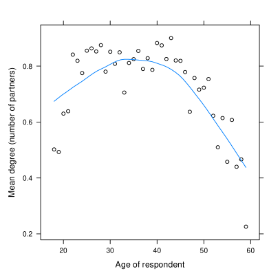
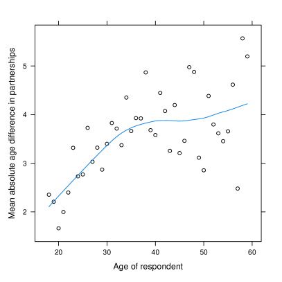
Figure 1: Mean number of partners reported by a respondent (left) and mean absolute difference between age of respondent and that of the respondent’s partner(s) (right), as a function of age

To reduce correlations and improve the numeric conditioning of the model, we center and scale the ages of actors to be between $-\frac{1}{2}$ and $+\frac{1}{2}$. The transformation used does not modify the model itself, only the coefficients. This results in the following ERGM statistics:

overall age effects

represented by the summing, over all the actors, the product of each actor’s number of partners and of each function of interest of that actor’s age:

$$g_{[13,14]}(y,x)=\left(\sum_{i=1}^{n}\left\lvert y_{i}\right\rvert\left(\sqrt{\frac{t_{i}-18}{60-18}}-\frac{1}{2}\right),\sum_{i=1}^{n}\left\lvert y_{i}\right\rvert\left(\frac{t_{i}-18}{60-18}-\frac{1}{2}\right)\right);$$

age difference effects

represented by the summing, over all the dyads, the product of the value of each dyad and of each function of interest of the incident actors’ ages:

$$g_{[15,16,17,18]}(y,x)=\left(\sum_{(i,j)\in\mathbb{Y}}y_{i,j}\left\lvert\sqrt{\frac{t_{i}-18}{60-18}}-\sqrt{\frac{t_{j}-18}{60-18}}\right\rvert^{p},\vphantom{\sum_{(i,j)\in\mathbb{Y}}y_{i,j}\left\lvert\frac{t_{i}-18}{60-18}-\frac{t_{j}-18}{60-18}\right\rvert^{p}}\right.\\ \left.\vphantom{\sum_{(i,j)\in\mathbb{Y}}y_{i,j}\left\lvert\sqrt{\frac{t_{i}-18}{60-18}}-\sqrt{\frac{t_{j}-18}{60-18}}\right\rvert^{p}}\sum_{(i,j)\in\mathbb{Y}}y_{i,j}\left\lvert\frac{t_{i}-18}{60-18}-\frac{t_{j}-18}{60-18}\right\rvert^{p}\right)_{p\in\{1,2\}}.$$

6.4 Simulation study design

We performed two simulation studies. Firstly, we compared parameter estimates for 400 egocentric bootstrapped resample sizes ranging from 600 to 12,000, logarithmically spaced. Secondly, we compared 100 resamples of each of the sizes 1,000, 6,000, and 11,000. For each sample size, we generated estimates as follows:

• Resample the desired numbers egos and their alters from the NHSLS dataset, as described in Section 6.2.

• Compute network statistics as described in Section 5.1.

• Fit an ERGM with terms and offset described in Section 6.3 using R (R Development Core Team, 2009) package statnet (Handcock et al., 2008).

• Record the ERGM parameter estimates $\hat{\theta}$.

In the framework of van Duijn, Gile, and Handcock (2009), we are considering networks of a given size with mean value parameters derived as described in Section 5, and consider whether the corresponding natural parameters, in the presence of an offset, are invariant to network size. A model with good invariance properties would thus produce natural parameter estimates that do not change substantially with a changing network size. The variability in the estimates due to bootstrap resampling provide a baseline for the magnitude of this change.

6.5 Results

We give the estimated model coefficients for the three-resample-size simulation in Table 5. The model parameter estimates are consistent with our expectations: same-sex partnership count has a significant negative coefficient, and there is a strong bias for monogamy for both sexes. Race homophily is consistently positive. The positive coefficient on the age asymmetry term indicates a bias for older-male-younger-female partnerships as well.

Table 5: Average bootstrap estimates (and standard errors) of NHSLS model parameters, by sample size

	$N=1000$	$N=6000$	$N=11000$
Term
Offset	$-6.91$ (fixed)	$-8.70$ (fixed)	$-9.31$ (fixed)
Actor activity by sex
Female	$-1.29$ $(0.88)$	$-1.10$ $(0.17)$	$-1.19$ $(0.13)$
Male	$-0.43$ $(0.91)$	$-0.58$ $(0.16)$	$-0.63$ $(0.12)$
Same-sex partnership	$-4.59$ $(1.75)$	$-4.07$ $(0.14)$	$-4.09$ $(0.11)$
Monogamy by sex
Female	$2.31$ $(0.33)$	$2.17$ $(0.11)$	$2.20$ $(0.08)$
Male	$2.00$ $(0.25)$	$1.93$ $(0.07)$	$1.94$ $(0.05)$
Actor activity by race
Black	$0$ (baseline)	$0$ (baseline)	$0$ (baseline)
Hispanic	$0.86$ $(0.35)$	$1.00$ $(0.13)$	$1.02$ $(0.11)$
Other	$1.28$ $(0.44)$	$1.39$ $(0.16)$	$1.42$ $(0.14)$
White	$0.51$ $(0.45)$	$0.58$ $(0.22)$	$0.60$ $(0.15)$
Race homophily by race
Black	$4.65$ $(0.60)$	$4.85$ $(0.27)$	$4.83$ $(0.18)$
Hispanic	$2.84$ $(0.48)$	$2.67$ $(0.22)$	$2.70$ $(0.16)$
Other	$3.34$ $(0.54)$	$3.20$ $(0.21)$	$3.17$ $(0.16)$
White	$2.11$ $(0.42)$	$2.09$ $(0.20)$	$2.13$ $(0.15)$
Age effects
$\sqrt{\text{age}}$ effect	$-1.71$ $(0.54)$	$-1.80$ $(0.24)$	$-1.74$ $(0.18)$
age effect	$1.62$ $(0.44)$	$1.65$ $(0.18)$	$1.60$ $(0.13)$
Age difference effects
Diff. in $\sqrt{\text{age}}$	$-8.29$ $(2.38)$	$-8.31$ $(1.21)$	$-8.19$ $(0.96)$
Diff. in age	$-7.70$ $(2.24)$	$-6.72$ $(1.05)$	$-6.61$ $(0.74)$
Squared diff. in $\sqrt{\text{age}}$	$4.37$ $(3.27)$	$4.08$ $(2.07)$	$3.72$ $(1.80)$
Squared diff. in age	$6.05$ $(2.98)$	$4.05$ $(1.51)$	$3.77$ $(1.11)$
Age-sex asymmetry	$0.98$ $(0.10)$	$0.94$ $(0.04)$	$0.95$ $(0.03)$

More importantly, the parameter estimates are essentially stable as the resampled network size ranges from 6,000 to 11,000. In fact, on average, the difference between a parameter’s estimate for 6,000 and 11,000 is smaller than 1 simulated standard error for that estimate based on resample size of 11,000. These standard errors are not conservative, since the original dataset is one third of that size and the resampling is reweighted, both of which lead to the standard errors in Table 5 being smaller than what the standard deviations of the parameter estimates would be in a hypothetical simple random sample of 11,000 egos. In short, the difference in the estimates due to the difference in network size is smaller than the differences due to sampling error.

The simulation of network sizes 600 through 12,000 shows a similar trend. We give the trends in the parameter estimates in Figure 2. The estimates show a pattern of asymptoting, although asymptoting for some of them — particularly age difference effects — appears to be slower. This could be an artifact of normalizing the ages.

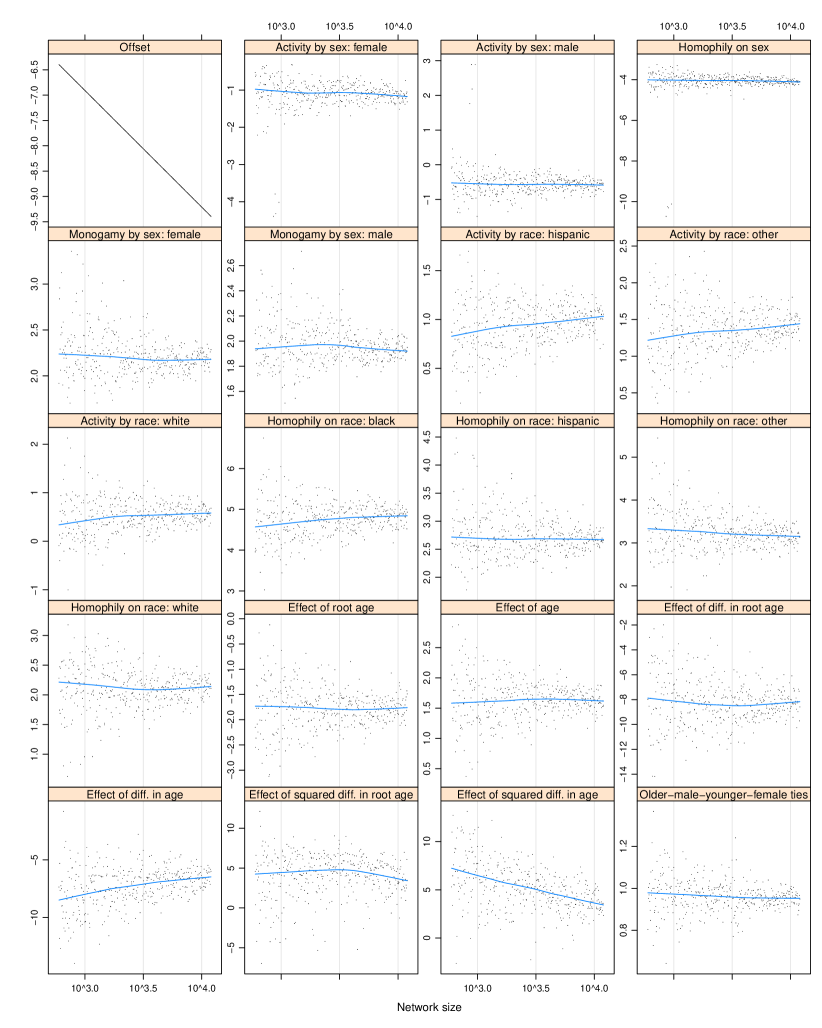
Figure 2: Parameter estimates of the model fit to the resamples of NHSLS dataset, as a function of network size, varying from 600 to 12,000, spaced logarithmically. Note that the horizontal axis is on a logarithmic scale.

All this suggests asymptotic invariance to network size for this, fairly complex, model. While limitations of computing capacity preclude computing parameter estimates for network sizes in the hundreds of millions — the population of the United States in 1992 in the age range surveyed — it is likely that these estimates would be very close to those for network size 12,000.

7 Discussion

Effect of network size and composition on ERGMs has received limited attention in the literature to date. We have described the desired behavior we would like a social network model to exhibit when applied to social networks of different sizes, and have shown which of these are (or are not) properties of an unadjusted ERGM. We propose a simple adjustment based on an offset term that appears to produce, asymptotically but also for networks of moderate size, the desired behavior: given that the network statistics are “local” in nature, the model produces the size appropriate mean statistics for group mixing and degree distributions under a variety of network sizes — similar distributions map to similar parameter values.

We demonstrated this property by fitting a fairly complex ERGM to networks of different sizes constructed to have similar structure.

We also described an approach to fitting ERGMs to egocentrically sampled data that makes use of our heuristics for similar structure across network sizes. Combined with the proposed network size adjustment for ERGMs, it may allow the parameter estimates from fitting the network data on a sample to be generalized to the population from which the sample was drawn.

This approach provides a principled framework for network comparison and simulation. With the offset adjustment, the remaining parameters in the ERGM can be used to test whether network structures represented in the model are statistically different between two networks, even if the networks have different size and/or composition. Since the parametrization is now size and composition invariant, this approach can also be used to simulate networks that have the same underlying structure, though they may have different size and composition.

Our analysis leaves open some questions. We limit our statistics to first- and second-order effects — dyadic and degree distribution effects — and do not discuss third-order effects such as triad-closure bias, and while two of the notions of locality that we describe allow modeling of such effects, we do not examine the properties of these in the presence of an offset, because the egocentrically sampled data available do not contain information about such effects. Goodreau et al. (2008), using dyad census data, fit a geometrically-weighted edgewise shared partner (GWESP) statistic (Snijders et al., 2006; Hunter and Handcock, 2006; Hunter, 2007), used to model triad-closure bias, and found that the coefficient of the GWESP statistic appeared to asymptote as school sizes increased. Other parameters, except for the overall density parameter, also did not appear to depend on school sizes (Goodreau, 2009). This suggests that our approach applies to third-order effects as well, but this is a subject for future research.

Another question is whether convergence to the asymptotic estimates could be sped up by modifying the offset term: $\left\lvert y\right\rvert\log\frac{1}{n}$ has the advantage of simplicity, but there are other candidates, such as $\left\lvert y\right\rvert\operatorname{logit}\left(\frac{\mu}{n-1}\right)$, for a constant $\mu\ll n$ that may have better properties. At the same time, if the sufficient statistics of the model or some linear combination thereof include $\left\lvert y\right\rvert$, the change in the offset coefficient will be absorbed only into their parameter estimates, and will not affect the convergence of the others. In our example, the number of partners of males and the number of partners of females sum to twice the number of edges, and, thus, their coefficients would play this role.

While we describe a way to use egocentrically sampled data to construct networks with similar structures but varying sizes, and describe how these parameter estimates may be generalized to the underlying network, we do not have an appropriate measure of uncertainty of these estimates — we note above that the standard errors we report for the larger network sizes are too small — rigorously assessing this uncertainty is a subject of ongoing work.

Lastly, network size can affect the structure of a network in ways other than density, and we do not explore these effects here.

Appendix

Appendix A Change statistics and Gibbs sampling

A.1 Conditional probability of a dyad $(i,j)$

ERGM distribution in (1) has the conditional probability of an edge at $(i,j)$, given the rest of the network, of

$$\operatorname{Pr}_{\eta,g}( Y_{i,j}=1|x,Y-(i,j)=y-(i,j);\theta)=$$

$$=\frac{\operatorname{Pr}_{\eta,g}(Y=y+(i,j)|N;\theta)}{\operatorname{Pr}_{\eta,g}(Y=y-(i,j)|N;\theta)+\operatorname{Pr}_{\eta,g}(Y=y+(i,j)|N;\theta)}$$

$$=\frac{\frac{\exp\left({\eta(\theta,x)}\cdot{g(y+(i,j),x)}\right)}{\cancel{c_{\eta,g}(\theta,x)}}}{\frac{\exp\left({\eta(\theta,x)}\cdot{g(y-(i,j),x)}\right)}{\cancel{c_{\eta,g}(\theta,x)}}+\frac{\exp\left({\eta(\theta,x)}\cdot{g(y+(i,j),x)}\right)}{\cancel{c_{\eta,g}(\theta,x)}}}$$

$$=\frac{1}{\exp\left({\eta(\theta,x)}\cdot{g(y-(i,j),x)}-{\eta(\theta,x)}\cdot{g(y+(i,j),x)}\right)+1}$$

$$=\frac{1}{1+\exp\left(-{\eta(\theta,x)}\cdot{\Delta_{i,j}g(y,x)}\right)}$$

$$=\operatorname{logit^{-1}}\left({\eta(\theta,x)}\cdot{\Delta_{i,j}g(y,x)}\right),$$

where $\operatorname{logit^{-1}}(x)\equiv\frac{1}{1+\exp\left(-x\right)}$ and $\Delta_{i,j}g_{k}(y,x)\equiv g_{k}(y+(i,j),x)-g_{k}(y-(i,j),x)$.

A.2 Naïve Gibbs sampling algorithm for ERGMs

The following algorithm can be used to generate a random draw from an ERGM probability distribution (1) with an intractable normalizing constant:

0:  Arbitrary $y^{0}\in\mathcal{Y}$ and $S$ sufficiently large

1:  for $s\leftarrow 1$ to $S$ do

2:     $(i,j)\leftarrow\text{{RandomChoose}}(\mathbb{Y})$

3:      $r\leftarrow\operatorname{logit^{-1}}\left({\eta(\theta,x)}\cdot{\Delta_{i,j}g(y,x)}\right)$ {i.e. $\operatorname{Pr}_{\eta,g}(Y_{i,j}=1|x,Y^{(s-1)}-(i,j)=y^{(s-1)}-(i,j);\theta)$}

4:     $u\leftarrow\operatorname{Uniform}(0,1)$

5:     if $u<r$ then

6:        $y^{s}\leftarrow y^{(s-1)}+(i,j)$ {Have a tie at $(i,j)$ with probability $r$.}

7:     else

8:        $y^{s}\leftarrow y^{(s-1)}-(i,j)$ {Have no tie at $(i,j)$ with probability $1-r$.}

9:  return  $y^{S}$

Here, $\text{{RandomChoose}}(A)$ is a function that, given a set, $A$, selects and returns a member $a\in A$ at random.

Appendix B Details of asymptotic properties of ERGMs

B.1 Size-invariant statistics of linear ERGMs

In this section, we prove the assertion about linear ERGMs that was stated in Section 3.3. Consider a sequence of random undirected networks $Y^{(n_{1})},Y^{(n_{2})},\dotsc$ of increasing size whose actor attributes $x^{(n)}$ such that frequency or distribution of any exogenous actor attributes converges as $n\to\infty$ — that is, the network size grows, but the composition does not change. Because we do not model actor attributes in this discussion, an intuitive way to construct such a sequence is by defining some initial set of actor attributes $x^{(n_{0})}$ and defining, for any integer $k>1$, $x^{(n_{k})}$ to simply be $x^{(n_{0})}$ replicated $k$ times.

Let $\eta(\theta,x^{(n)})=\theta$ be the natural parameter vector (i.e. a linear ERGM); $g(\cdot,\cdot)$ be a vector of network statistics that may also depend on network size and composition; and $T(\cdot,\cdot)$ be the vector of network statistics, which may depend on network size and composition, but whose expected value needs to remain constant as network size changes or converge to a finite limit as it increases.

Suppose that for some $T(\cdot,\cdot)$ of interest,

$$\exists_{g(\cdot,\cdot)}\forall_{\theta}\forall_{\epsilon>0}\exists_{N<\infty}\forall_{n>N,n^{\prime}>N}\left\lvert\sum_{y\in\mathcal{Y}^{(n)}}T(y,x^{(n)})\frac{\exp\left(\theta\cdot g(y,x^{(n)})\right)}{c_{\eta,g}(\theta,x^{(n)})}-\vphantom{\sum_{y\in\mathcal{Y}^{(n^{\prime})}}T(y,x^{(n^{\prime})})\frac{\exp\left(\theta\cdot g(y,x^{(n^{\prime})})\right)}{c_{\eta,g}(\theta,x^{(n^{\prime})})}}\right.\\ \left.\vphantom{\sum_{y\in\mathcal{Y}^{(n)}}T(y,x^{(n)})\frac{\exp\left(\theta\cdot g(y,x^{(n)})\right)}{c_{\eta,g}(\theta,x^{(n)})}-}\sum_{y\in\mathcal{Y}^{(n^{\prime})}}T(y,x^{(n^{\prime})})\frac{\exp\left(\theta\cdot g(y,x^{(n^{\prime})})\right)}{c_{\eta,g}(\theta,x^{(n^{\prime})})}\right\rvert<\epsilon.$$ (6)

That is, suppose that for this particular $T(\cdot,\cdot)$, there exists a vector of statistics $g(\cdot,\cdot)$ such that for any given fixed value of natural parameter vector $\theta$, the maximum difference in expected value of the statistic of interest $T(\cdot,\cdot)$ due to differences in network size can be made arbitrarily small for sufficiently large networks. Then (Strichartz, 2000, p. 71)

$$\exists_{g(\cdot,\cdot)}\forall_{\theta}\lim_{n\to\infty}\sum_{y\in\mathcal{Y}^{(n)}}T(y,x^{(n)})\frac{\exp\left(\theta\cdot g(y,x^{(n)})\right)}{c_{\eta,g}(\theta,x^{(n)})}=t_{g}(\theta,X)<\infty:$$ (7)

the expected value converges to some $t_{g}(\theta,X)$, a function of $\theta$ and asymptotic network composition distribution $X$. For this particular combination of $g(\cdot,\cdot)$ and $T(\cdot,\cdot)$, (7) holds for all $\theta$, and therefore holds for $\theta=0$. But then,

$$\lim_{n\to\infty}\sum_{y\in\mathcal{Y}^{(n)}}T(y,x^{(n)})\frac{\exp\left(0\cdot g(y,x^{(n)})\right)}{c_{\eta,g}(0,x^{(n)})}=t_{g}(0,X),$$

$$\lim_{n\to\infty}\sum_{y\in\mathcal{Y}^{(n)}}T(y,x^{(n)})\frac{1}{\sum_{y^{\prime}\in\mathcal{Y}_{n}}1}=t_{g}(0,X),$$

$$\lim_{n\to\infty}\frac{1}{\left\lvert\mathcal{Y}^{(n)}\right\rvert}\sum_{y\in\mathcal{Y}^{(n)}}T(y,x^{(n)})=t_{g}(0,X).$$

This summation is just the expected value of $T(\cdot,\cdot)$ under an Erdős-Rényi graph of that size and composition with each dyad value having an independent $\operatorname{Bernoulli}\left(\frac{1}{2}\right)$ distribution, with $x^{(n)}$ being irrelevant, so

$$\lim_{n\to\infty}\operatorname{E}\left(T(Y,x^{(n)})\right)=t_{g}(0,X)$$

where $Y$ is a $\operatorname{Bernoulli}\left(\frac{1}{2}\right)$ graph of size $n$.

Thus, regardless of what $g(\cdot,\cdot)$ may be, unless $T(y,x^{(n)})$ already has the property of its expectation converging as its network size increases (at least in a Bernoulli model), it is not possible to construct an ERGM that satisfies (6). In particular, the expected mean degree in an undirected $\operatorname{Bernoulli}(\frac{1}{2})$ graph of size $n$ is $\frac{n-1}{2}\to\infty$ as $n\to\infty$, so the degree distribution does not remain unaffected or converge under changing network size. The network statistics that can be made unaffected by network size include the density of the network, the densities of subnetworks, and affine transformations thereof with fixed coefficients.

B.2 Asymptotic degree distribution of a simple offset model

Starting with (2), let

$$p_{n}=\operatorname{Pr}_{\eta,g}(Y_{i,j}^{(n)}=1|x^{(n)};\theta)=\operatorname{logit^{-1}}\left(-\log n+\theta\right).$$

Then,

$$\lim_{n\to\infty} \operatorname{Pr}_{\eta,g}(|Y^{(n)}_{i}|=d|x^{(n)})$$

$$=\lim_{n\to\infty}\binom{n-1}{d}\left({p_{n}}\right)^{d}\left(1-{p_{n}}\right)^{n-1-d}$$

$$=\lim_{n\to\infty}\frac{(n-1)!}{(n-1-d)!d!}\left(\exp\left(\operatorname{logit}{p_{n}}\right)\right)^{d}\left(1-{p_{n}}\right)^{n-1}$$

$$=\lim_{n\to\infty}\frac{\prod_{k=1}^{d}(n-k)}{d!}\left(\exp\left(-\log n+\theta\right)\right)^{d}$$

$$\phantom{=\lim_{n\to\infty}}\times\left(1-\frac{1}{1+n\exp\left(-\theta\right)}\right)^{n}\left(1-\frac{1}{1+n\exp\left(-\theta\right)}\right)^{-1}$$

$$=\lim_{n\to\infty}\left(\prod_{k=1}^{d}\frac{n-k}{n}\right)\frac{1}{d!}\left(\exp\left(\theta\right)\right)^{d}$$

$$\phantom{=\lim_{n\to\infty}}\times\left(1+\frac{\exp\left(\theta\right)}{n}\right)^{-n}\left(1-\frac{1}{1+n\exp\left(-\theta\right)}\right)^{-1}$$

$$=\frac{1}{d!}\left(\exp\left(\theta\right)\right)^{d}\exp\left(-\exp\left(\theta\right)\right),$$

the PDF of a Poisson distribution with mean $\exp\left(\theta\right)$.

References

- Admiraal (2009) Ryan Admiraal. Dynamic Network Models based on Revealed Preference for observed relations and Egocentric Data. PhD thesis, University of Washington, Seattle, WA, 2009.
- Anderson et al. (1999) Brigham S. Anderson, Carter Butts, and Kathleen Carley. The interaction of size and density with graph-level indices. Social Networks, 21(3):239–267, 1999. ISSN 0378-8733. doi: 10.1016/S0378-8733(99)00011-8.
- Davison and Hinkley (1997) Anthony C. Davison and David V. Hinkley. Bootstrap methods and their application. Cambridge University Press, Cambridge, 1997. ISBN 0-521-57391-2. URL http://statwww.epfl.ch/davison/BMA/.
- Frank and Strauss (1986) Ove Frank and David Strauss. Markov graphs. Journal of The American Statistical Association, 81(395):832–842, 1986.
- Goodreau (2009) Steven M. Goodreau. Results of analyses performed for Goodreau et al. (2008) that were not published in that article. Personal communication, 2009.
- Goodreau et al. (2008) Steven M. Goodreau, James Kitts, and Martina Morris. Birds of a feather, or friend of a friend? Using exponential random graph models to investigate adolescent social networks. Demography, 45(1):103–125, February 2008.
- Hamilton et al. (2008) Deven T. Hamilton, Mark S. Handcock, and Martina Morris. Degree distributions in sexual networks: A framework for evaluating evidence. Sexually Transmitted Diseases, 35:30–40, 2008.
- Handcock et al. (2008) Mark S. Handcock, David R. Hunter, Carter T. Butts, Steven M. Goodreau, and Martina Morris. statnet: Software tools for the representation, visualization, analysis and simulation of network data. Journal of Statistical Software, 24(1):1–11, May 2008. ISSN 1548-7660. URL http://www.jstatsoft.org/v24/i01.
- Helleringer and Kohler (2007) Stéphanie Helleringer and Hans-Peter Kohler. Sexual network structure and the spread of HIV in Africa: evidence from Likoma Island, Malawi. AIDS, 21(17):2323–2332, 2007.
- Holland and Leinhardt (1981) Paul W. Holland and Samuel Leinhardt. An exponential family of probability distributions for directed graphs. Journal of The American Statistical Association, 76(373):33–65, 1981.
- Hunter (2007) David R. Hunter. Curved exponential family models for social networks. Social Networks, 29:216–230, 2007. ISSN 0378-8733.
- Hunter and Handcock (2006) David R. Hunter and Mark S. Handcock. Inference in curved exponential family models for networks. Journal of Computational & Graphical Statistics, 15(3):565–583, 2006.
- Klovdahl et al. (1994) Alden S. Klovdahl, John J. Potterat, Donald E. Woodhouse, Muth John B., Stephen Q. Muth, and William W. Darrow. Social networks and infectious disease: the Colorado Springs study. Social Science & Medicine, 38(1):79, 1994.
- Koehly et al. (2004) Laura M. Koehly, Steven M. Goodreau, and Martina Morris. Exponential family models for sampled and census network data. Sociological Methodology, 34(1):241–270, 2004.
- Laumann et al. (1992) Edward O. Laumann, John H. Gagnon, Robert T. Michael, and Stuart Michaels. National health and social life survey. Chicago, IL, USA: University of Chicago and National Opinion Research Center [producer], 1995. Ann Arbor, MI, USA: Inter-university Consortium for Political and Social Research [distributor], 2008-04-17, 1992. Computer file.
- Laumann et al. (1994) Edward O. Laumann, John H. Gagnon, Robert T. Michael, and Stuart Michaels. The social organization of sexuality. University of Chicago Press, Chicago, 1994. ISBN 0226469573.
- Leskovec et al. (2007) Jure Leskovec, J. Kleinberg, and C. Faloutsos. Graph evolution: Densification and shrinking diameters. In ACM Transactions on Knowledge Discovery from Data (TKDD), pages 1–41. ACM Press New York, NY, USA, 2007.
- McCullagh and Nelder (1989) Peter McCullagh and John A. Nelder. Generalized Linear Models, volume 37 of Monographs on Statistics and Applied Probability. Chapman & Hall/CRC, second edition, August 1989. ISBN 0-412-31760-5.
- McPherson et al. (2001) Miller McPherson, Lynn Smith-Lovin, and James M. Cook. Birds of a feather: Homophily in social networks. Annual Review of Sociology, 27(1):415–444, 2001.
- Morris (1991) Martina Morris. A log-linear modeling framework for selective mixing. Mathematical Biosciences, 107(2):349–77, 1991.
- Morris and Kretzschmar (1997) Martina Morris and Mirjam Kretzschmar. Concurrent partnerships and the spread of HIV. AIDS, 11(5):641–648, April 1997.