Mean-field study of itinerant ferromagnetism in trapped ultracold Fermi gases: Beyond the local density approximation

Abstract

We theoretically investigate the itinerant ferromagnetic transition of a spherically trapped ultracold Fermi gas with spin imbalance under strongly repulsive interatomic interactions. Our study is based on a self-consistent solution of the Hartree-Fock mean-field equations beyond the widely used local density approximation. We demonstrate that, while the local density approximation holds in the paramagnetic phase, after the ferromagnetic transition it leads to a quantitative discrepancy in various thermodynamic quantities even with large atom numbers. We determine the position of the phase transition by monitoring the shape change of the free energy curve with increasing the polarization at various interaction strengths.

I Introduction

Recent experimental progress with Feshbach resonances in ultracold atomic Fermi gases has created opportunities to investigate long-standing many-body problems in condensed matter physics. One interesting issue is the problem of itinerant ferromagnetism in two-component (spin-1/2) Fermi gases with repulsive interactions. The study of itinerant ferromagnetism in condensed matter physics is a fundamental problem which has an extensive history, dating back to the basic model proposed by Stoner StonerPRSLA1938 . However, the phase transition theory of itinerant ferromagnetism is still qualitative. It is thought that a Fermi gas with repulsive interactions may simulate the Stoner model and therefore could undergo a ferromagnetic phase transition to a spin-polarized state with increased interaction strength Salasnich2000 ; SogoPRA2002 ; MacDonald2005PRL ; WuPreprint ; LeBlancPRA09 . This is a result of the competition between the repulsive interaction and the Pauli exclusion principle. The former tends to induce polarization, to reduce the interaction energy, while the latter prefers a balanced system with equal spin populations – and hence a reduced kinetic energy. Above a critical interaction strength, the reduced interaction energy for a polarized Fermi gas will overcome the gain in kinetic energy. Hence, a ferromagnetic phase transition should occur. Itinerant ferromagnetism is therefore a purely quantum-mechanical effect which occurs when the minimum energy is at nonzero magnetization, due to the Pauli principle.

Recently, an experimental group reported progress in this direction ketterle2009Science , which has attracted intense theoretical interest LeBlancPRA09 ; Conduit2009a ; Conduit2009b ; Zhai ; Fregoso2009 ; Cui2010 ; Spilati ; Chang . By using a non-adiabatic field switch to the upper branch of a Feshbach resonance with a positive s-wave scattering length $a_{s}>0$, the experimentalists realized a two-component “repulsive” Fermi gas of ⁶Li atoms in a harmonic trap, despite the fact that the lower branch of the Feshbach resonance is a molecule where the fermions attract each other. Initial evidence attributed to a ferromagnetic phase transition has been observed, suggesting that the transition takes place at $k_{F}^{0}a_{s}\simeq 2.2$, where $k_{F}^{0}$ is the Fermi vector of an ideal gas at the trap center. Earlier experiments measuring interaction energies Salomon also provide qualitative evidence in this direction.

For a trapped Fermi gas, many physical quantities may be used to characterize the ferromagnetic phase transition. The most direct one is the density profile of each component. It was suggested from mean-field theory that with a large scattering length, the two Fermi components in a trap should become spatially separated Salasnich2000 ; SogoPRA2002 . This would imply that the majority component stays at the trap center and the minority is repelled to the trap edge. This spatial inhomogeneity is evidence of a ferromagnetic phase. However, these inhomogeneous density profiles or spin domains were not observed in the recent experiments, which is away from thermal equilibrium due to the dynamical use of the upper branch of Feshbach resonances. For such a non-equilibrium state, the onset of phase transition is better characterized by a suppression of inelastic three-body collisions, together with a minimum in kinetic energy, and a maximum in cloud size. From this evidence, a phase transition was experimentally identified at a critical scattering length of $k_{F}^{0}a_{s}\simeq 2.2$ and a temperature of $T\simeq 0.12T_{F}$.

On the theoretical side, itinerant ferromagnetism is difficult to treat quantitatively. The phase transition occurs at large interaction strengths, where fluctuations can be huge. Currently, even the critical interaction strength for the transition is still under debate. For a homogeneous gas, mean-field theory predicts a zero-temperature critical value $k_{F}a_{s}=\pi/2$ StonerPRSLA1938 , while a second-order perturbative calculation MacDonald2005PRL predicts a much lower critical coupling strength of $k_{F}a_{s}\sim 1.054$. More accurate quantum Monte Carlo simulations recently reported even lower critical values $k_{F}a_{s}\simeq 0.8$ Conduit2009b ; Spilati ; Chang . For the experimental situation with harmonic traps, a local density approximation (LDA) is extensively used in order to average over the entire trap. At zero temperature, the LDA calculation within the mean-field theory predicts $k_{F}^{0}a_{s}\simeq 1.84$. A finite but low temperature causes an increase of the critical interaction strength. At the lowest accessible temperature in the recent experiments ($T\simeq 0.12T_{F}$), we found that the LDA predicts $k_{F}^{0}a_{s}\simeq 1.93$.

In this paper, rather than addressing the challenging problem of calculating the critical interaction strength, we instead examine the validity of the widely used local density approximation, by solving the Hartree-Fock mean-field equations self-consistently for a trapped imbalanced Fermi gas. The LDA is believed to be applicable in general cases. However, in extreme conditions such as a spin-imbalanced superfluid Fermi gas in a strongly anisotropic trap, it necessarily breaks down due to the strongly distorted superfluid-normal interface, which gives a large surface energy Silva ; Imambekov ; Liu2007PRA . The same situation could arise in the spatially phase-separated ferromagnetic phase. In this respect, while the mean-field approximation used in this work is not exact, our examination of the LDA may provide useful insight for future applications of the LDA to more accurate homogeneous equations of state of a repulsive Fermi gas. On the other hand, beyond-LDA corrections were recently considered by LeBlanc and co-workers through the phenomenological inclusion of a surface energy term LeBlancPRA09 . Our study may be used to determine accurately the phenomenological parameters as an input.

Our main results may be summarized in the following. First, we find a notable disagreement between the self-consistent Hartree-Fock solution and the LDA result in the strongly interacting ferromagnetic phase where the two species are spatially separated, even with large atom number up to $10^{5}$. This discrepancy arises from the non-negligible surface energy, which become increasingly important at large interaction strength. Secondly, we calculate various thermodynamic quantities at different temperatures and spin polarizations. The obtained kinetic energy, interaction energy, and the atomic loss rate all exhibit a turning point as an indication for the ferromagnetic phase transition. We also examine the shape change of the free-energy curves as a function of spin polarization with increasing the interaction strength, from which we are able to determine accurately a mean-field critical interaction strength. We find that this does agree with the LDA prediction, presumably because surface terms play a smaller role at these interaction strengths.

The rest of the paper is organized as follows. In Sec. II, we briefly outline the model and the Hartree-Fock mean-field approach. In Sec. III, we present a detailed comparison of our results with that obtained from the mean-field LDA, as well as a detailed analysis for various thermodynamic quantities. Sec. IV is devoted to the conclusions and further remarks.

II Methods

We consider an imbalanced Fermi gas with unequal spin populations in a spherically trap with an effective repulsive interaction, as a minimum model for these experiments. The system may be described by the Hamiltonian,

$${\cal H=}\sum_{\sigma}\int d{\bf r}\hat{\Psi}_{\sigma}^{\dagger}\left({\bf r}\right)H_{\sigma}^{s}\hat{\Psi}_{\sigma}\left({\bf r}\right)+U\int d{\bf r}\hat{\Psi}_{\uparrow}^{\dagger}\hat{\Psi}_{\downarrow}^{\dagger}\hat{\Psi}_{\downarrow}\hat{\Psi}_{\uparrow},$$ (1)

where the pseudo-spin $\sigma=\uparrow,\downarrow$ denotes different hyperfine states and $\hat{\Psi}_{\sigma}\left({\bf r}\right)$ is the annihilation Fermi field operator for the spin-$\sigma$ state. The single-particle Hamiltonian $H_{\sigma}^{s}=-\hbar^{2}\nabla^{2}/(2m)+V\left({\bf r}\right)-\mu_{\sigma}$ and $V\left({\bf r}\right)=m\omega^{2}r^{2}/2$ is an isotropic harmonic trapping potential with frequency $\omega$. The effective repulsive interaction strength is $U=4\pi\hbar^{2}a_{s}/m>0$ in the lowest Born approximation. The total number of fermions and the number difference in different hyperfine states are, respectively, $N=N_{\uparrow}+N_{\downarrow}$ and $\delta N=N_{\uparrow}-N_{\downarrow}$. We have introduced different chemical potentials, $\mu_{\uparrow,\downarrow}=\mu\pm\delta\mu$, to account for the number difference or population imbalance.

We use the Hartree-Fock mean-field (MFA) approximation to solve the Hamiltonian, which amounts to decoupling the interaction term $\hat{\Psi}_{\uparrow}^{\dagger}\hat{\Psi}_{\downarrow}^{\dagger}\hat{\Psi}_{\downarrow}\hat{\Psi}_{\uparrow}=n_{\uparrow}\left({\bf r}\right)\hat{\Psi}_{\downarrow}^{\dagger}\hat{\Psi}_{\downarrow}+n_{\downarrow}\left({\bf r}\right)\hat{\Psi}_{\uparrow}^{\dagger}\hat{\Psi}_{\uparrow}-n_{\uparrow}\left({\bf r}\right)n_{\downarrow}\left({\bf r}\right)$. Here, $n_{\sigma}\left({\bf r}\right)=<\hat{\Psi}_{\sigma}^{\dagger}\hat{\Psi}_{\sigma}>$ is the density. The Heisenberg equation of motion for $\hat{\Psi}_{\sigma}\left({\bf r}\right)$ then reads

$$i\hbar\partial_{t}\hat{\Psi}_{\sigma}=\left[-\frac{\hbar^{2}}{2m}\nabla^{2}+V\left({\bf r}\right)+Un_{\overline{\sigma}}\left({\bf r}\right)-\mu_{\sigma}\right]\hat{\Psi}_{\sigma}.$$ (2)

We solve the equations of motion by expanding $\hat{\Psi}_{\sigma}\left({\bf r}\right)=\sum_{j}u_{j\sigma}\left({\bf r}\right)\hat{c}_{j\sigma}\exp\left[-iE_{j\sigma}t\right]$, where the field operator $\hat{c}_{j\sigma}$ annihilates a spin-$\sigma$ fermion in state $j$ with wave function $u_{j\sigma}\left({\bf r}\right)$ and energy $E_{j\sigma}$. This yields the single-particle Schrodinger equation,

$$\left[-\frac{\hbar^{2}}{2m}\nabla^{2}+V\left({\bf r}\right)+Un_{\overline{\sigma}}\left({\bf r}\right)-\mu_{\sigma}\right]u_{j\sigma}=E_{j\sigma}u_{j\sigma},$$ (3)

where $u_{j\sigma}\left({\bf r}\right)$ are normalized as $\int d^{3}{\bf r}|u_{j\sigma}|^{2}=1$. The density distribution $n_{\sigma}\left({\bf r}\right)$ of spin-$\sigma$ species can be written as

$$n_{\sigma}\left({\bf r}\right)=\sum_{j}|u_{j\sigma}\left({\bf r}\right)|^{2}f\left(E_{j\sigma}\right),$$ (4)

where $f\left(x\right)=1/\left[\exp\left(\beta x\right)+1\right]$ is the Fermi distribution function at an inverse temperature of $\beta=1/(k_{B}T)$. The chemical potential is determined through the number of atoms for the two species:

$$\int d{\bf r}n_{\sigma}\left({\bf r}\right)=N_{\sigma}.$$ (5)

We self-consistently solve the coupled equations (3)-(5). For computational reasons, we introduce a high-energy cut-off $E_{c}$ to truncate the summation in the density equation (4). For high-lying modes with $E>E_{c}$, we then adopt a semi-classical approximation by assuming that the wavefunction $u_{j\sigma}$ is locally a plane wave. We refer to refs. Liu2007PRA and Reidl1999PRA for details. The density profile can therefore be written in the form,

$$n_{\sigma}\left(r\right)=\sum_{E_{nl}^{\sigma}<E_{c}}\frac{2l+1}{4\pi r^{2}}|u_{nl}^{\sigma}|^{2}f\left(E_{nl}^{\sigma}\right)+\int_{E_{c}}^{\infty}d\epsilon\xi_{\sigma}f\left(\epsilon\right),$$ (6)

where $\xi_{\sigma}=m\sqrt{\epsilon+\mu_{\sigma}-V\left(r\right)-Un_{\overline{\sigma}}\left(r\right)}/\left(2\pi^{2}\hbar^{2}\right)$ and $u_{nl}^{\sigma}\left(r\right)$ is the radial wavefunction. For the given numbers of atoms $N$ and $\delta N$, temperature $T$, and s-wave scattering length $a_{s}$, our self-consistent iterative procedure runs as follows: (i) Start with a Thomas-Fermi profile for the density distribution of each species or the previous determined density distribution $n_{\sigma}\left(r\right)$; (ii) Solve the equation (3) for all the radial wave functions $u_{nl}^{\sigma}(r)$ with energy levels below the cutoff $E_{c}$; (iii) Calculate the new density profiles, adding both contributions from low-lying modes and high-lying modes; (iv) Update the chemical potentials according to the number equation (5) and (v )finally check the convergence by comparing the old and new density profiles. The above steps are repeated until the difference in the old and new density profiles decreases to an acceptable level. We note that the value of the high-energy cutoff should be carefully examined so that the numerical results are independent of the choice of $E_{c}$.

For the thermodynamic properties, we determine the entropy $S$ straightforwardly by

$$S=-k_{B}\sum_{nl\sigma}\left(2l+1\right)f\left(E_{nl}^{\sigma}\right)\ln f\left(E_{nl}^{\sigma}\right),$$ (7)

where the summation is restricted to the low-lying modes below the cutoff $E_{c}$, as the contribution from the high-lying modes is exponentially small. We also calculate the total energy $E$ using

$$E = \sum_{\sigma}\left[\sum_{E_{nl}^{\sigma}<E_{c}}E_{nl}^{\sigma}f\left(E_{nl}^{\sigma}\right)+\int d{\bf r}\int_{E_{c}}^{\infty}d\epsilon\epsilon\xi_{\sigma}f\left(\epsilon\right)\right]$$ (8)

$$+U\int dr4\pi r^{2}n_{\uparrow}\left(r\right)n_{\downarrow}\left(r\right)+\sum_{\sigma}\mu_{\sigma}N_{\sigma}.$$

The free energy at finite temperatures is obtained by using $F=E-TS$.

Experimentally, the kinetic energy $E_{{\rm ki}n}$ can be obtained by measuring the radial width of the ultra-cold gas, after free expansion without a trapping potential or Feshbach magnetic field. In our numerical work, we calculate the kinetic energy by subtracting from the total energy the potential energy $E_{{\rm pot}}=\int d{\bf r}V\left({\bf r}\right)n\left({\bf r}\right)$ and the interaction energy $E_{{\rm int}}=U\int d{\bf r}n_{\uparrow}\left({\bf r}\right)n_{\downarrow}\left({\bf r}\right)$, namely, $E_{{\rm ki}n}=E-E_{{\rm pot}}-E_{{\rm int}}$. Another observable quantity is the three-body loss rate, which, in the weakly interacting regime, may be estimated by the expression Petrov2003PRA ,

$$\Gamma=\Gamma_{0}\lambda^{6}\int d\mathbf{r}n_{\uparrow}\left(r\right)n_{\downarrow}\left(r\right)n\left(r\right).$$ (9)

Here $\lambda=k_{F}^{0}a_{s}$ and $n\left(r\right)=n_{\uparrow}\left(r\right)+n_{\downarrow}\left(r\right)$. The prefactor $\Gamma_{0}$ may be determined theoretically. While its detailed value is not of interest in determining the ferromagnetic phase transition, we note that $\Gamma_{0}$ depends on the scattering length and Feshbach resonance properties. As this is a low-density approximation, finite density effects must also be taken into account in interpreting three-body loss data as a guide to atomic density and polarization.

III Results and Discussions

In the numerical calculations, we use the “trap units” $\hbar=m=\omega=k_{\mathrm{B}}=1$. The length, energy and temperature are then measured in units of $a_{ho}=\left[\hbar/\left(m\omega\right)\right]^{1/2}$, $\hbar\omega$ and $\hbar\omega/k_{B}$, respectively. Furthermore, we will scale our results using characteristic quantities obtained from a zero-temperature ideal balanced Fermi gas in an isotropic harmonic trap. These are the Fermi energy $E_{F}=\left(3N\right)^{1/3}\hbar\omega$, Fermi temperature $T_{F}=E_{F}/k_{B}$, Thomas-Fermi radius $r_{TF}=\left(24N\right)^{1/6}a_{ho}$ and the peak density $n_{TF}=\left(6N\right)^{1/2}/3\pi^{2}a_{ho}^{-3}$. In most cases, we set the total atom number $N=10^{5}$ and temperature $T=0.12T_{F}$, comparable to the parameters used in the recent MIT experiment. To remove complications due to spin degeneracy, we also set a small polarization $p=(N_{\uparrow}-N_{\downarrow})/N=0.10$. We use a cut-off energy $E_{c}=85\hbar\omega$ and solve the Hartree-Fock mean-field equation within the subspace $n_{\mathrm{max}}=80$ and $l_{\mathrm{max}}=120$, which contains all the energy levels with energy $E<E_{c}$.

In the following, we first compare the Hartree-Fock mean-field density profiles with the corresponding LDA predictions to examine the validity of LDA. We then investigate in detail some thermodynamic properties and determine the critical interaction strength for emergence of the ferromagnetic state.

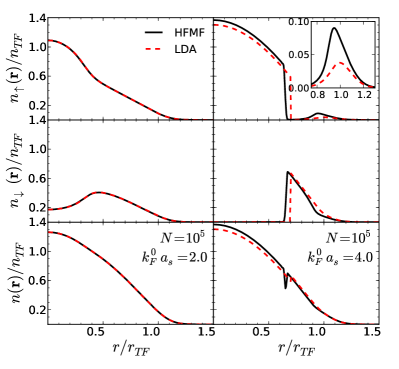
Figure 1: (Color online) Spin-up, spin-down and total density profiles of an imbalanced Fermi gas at $k_{F}^{0}a_{s}=2.0$ (left column) and $k_{F}^{0}a_{s}=4.0$ (right column). The solid and dashed lines refer to the Hartree-Fock MF and LDA results, respectively. The inset in the upper, right-column plot highlights the spin-up density profile at the trap edge. The spin polarization is $p=0.10$ and the number of atoms is $N=10^{5}$.

III.1 Hartree-Fock MF versus LDA

In Fig. 1, we present the density profile of each spin component and the total density profile of the imbalanced Fermi gas, calculated from Hartree-Fock MF (solid lines) and LDA (dashed lines) methods with total atom number $N=10^{5}$ and polarization $p=(N_{\uparrow}-N_{\downarrow})/N=0.10$ at $T=0.12T_{F}$. When the interaction strength is relatively weak (e.g., before the ferromagnetic phase transition, $k_{F}^{0}a_{s}=2.0$, left column), the LDA prediction agrees fairly well with that from the Hartree-Fock MF theory. Similar excellent agreement is also found in all the physical quantities that we have considered, including the chemical potential, energy, and the atom loss rate (see, for example, Fig. 3). However, when the repulsive interaction is stronger than a critical value (e.g., $k_{F}^{0}a_{s}=4.0$, right column), there is a significant discrepancy. In this parameter space, we observe a spatial phase separation in the density profiles, with majority spin-up atoms occupying the inner core and minority spin-down atoms repelled to the edge of the trap. This density separation is revealed clearly by both the LDA calculations and the Hartree-Fock MF calculations. However, LDA predicts a sudden change of the density profile of each spin component at $r\simeq 0.7r_{TF}$, due to the neglect of the spatial derivatives of the densities. At this point, the LDA necessarily fails and one has to resort to the more reliable self-consistent Hartree-Fock theory. Another notable discrepancy between LDA and Hartree-Fock MF comes from the trap edge $r\sim r_{TF}$, where the Hartree-Fock MF theory gives a much larger spin-up density than the LDA (see, for example, the inset in the right, upper plot). This is a well-known breakdown of the LDA method due to small densities occurring at the trap edge. Because of this failure, as we shall see, the LDA predicts a much smaller atom loss rate than the Hartree-Fock method. We note also that, for $r\sim r_{TF}$ the density of both two species becomes very low. There is no spatial phase separation, as a result of much weaker effective repulsive interactions.

We have also checked a smaller Fermi cloud with $N=10^{3}$ at the same temperature and polarization. As anticipated, the difference between Hartree-Fock MF and LDA becomes even more significant.

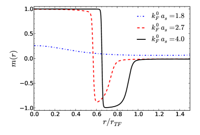
Figure 2: (Color online) Magnetization profile or local spin polarization at different interaction strengths: $k_{F}^{0}a_{s}=1.8$ (dash-dotted line), $2.7$ (dashed line), and $4.0$ (solid line). These curves are calculated using the Hartree-Fock MF theory for a total number of atoms $N=10^{5}$ and a polarization $p=0.10$ at $T=0.12T_{F}$.

III.2 Magnetization profile

As shown above, to reliably characterize the spin density or spin domains in the ferromagnetic phase, one must include corrections beyond-LDA by considering surface energy. This was done in the ref. LeBlancPRA09 by phenomenologically including a magnetization gradient term.

In Fig. 2, we report the Hartree-Fock MF results for the magnetization profile, $m\left(r\right)=(n_{\uparrow}\left(r\right)-n_{\uparrow}\left(r\right))/n\left(r\right)$. Before the transition ($k_{F}^{0}a_{s}=1.8$), the magnetization is nonzero but small. When the repulsive interaction is larger than the critical value ($k_{F}^{0}a_{s}=2.7$ and $4.0$), we find a fully magnetized core, whose size increases with increasing the interaction strength. As the strength increases, another nearly fully magnetized domain forms in the vicinity of the trap edge with $m\left(r\right)\approx-1$. These observations are in qualitative agreement with the theoretical predictions reported in ref. LeBlancPRA09 .

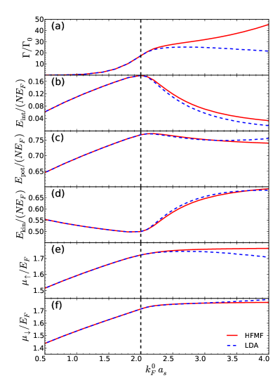
Figure 3: (Color online) Atom loss rate (a), interaction energy (b), potential energy (c), kinetic energy (d), and chemical potentials (e and f) as a function of interaction strength. The Hartree-Fock MF results (solid lines) are compared with the LDA predictions (dashed lines). The vertical dashed line marks the ferromagnetic phase transition. Here, $N=10^{5}$ , $p=0.10$, and $T=0.12T_{F}$.

III.3 Thermodynamic properties

We now turn to thermodynamic properties of the imbalanced Fermi gas with repulsive interactions, and compare our results with the experimental measurements where available. In Fig. (3), we show the atom loss rate (a), interaction energy (b), potential energy (c), kinetic energy (d) and chemical potentials (e and f). It is readily seen that LDA and Hartree-Fock MF calculations agree extremely well with each other for relatively weak interactions below the critical interaction strength ($k_{F}^{0}a_{s}\sim 2.0$), as mentioned earlier. However, the agreement tends to be worse as the interaction strength becomes stronger.

The most significant discrepancy occurs in the atom loss rate of three-body inelastic collisions. In the Hartree-Fock MF calculation, the loss rate increases monotonically with increasing interaction strength. While in the LDA calculations, it increases first but then decreases when the interaction strength is above the critical value, as illustrated in Fig. (3a). This discrepancy lies in the different prediction of the density tail from the two methods. It is clear that the loss rate is proportional to the integrated density profile overlap $n_{\uparrow}\left(r\right)n_{\downarrow}\left(r\right)$$\left(n_{\uparrow}\left(r\right)+n_{\downarrow}\left(r\right)\right)$ over the entire space. For strong repulsion, the spin-up and spin-down density profiles are essentially not overlapping (i.e., spatially phase separated), apart from the small regions at the phase-separation boundary, where the Hartree-Fock MF calculation shows a residue overlap, and at the edge of the trap, where due to the small density, the effective repulsion cannot sustain the phase separation further. The atom loss therefore arises mostly at the phase-separation boundary and at the trap edge. In these two regions, the LDA fails to give a quantitative density distribution and hence a reliable prediction for the atom loss rate.

However, it should be noted that, the qualitative experimental observation ketterle2009Science , the suppression of the atom loss rate at large repulsion, agrees with the LDA predictions, but is in contradiction with our more accurate Hartree-Fock MF calculations. We attribute the discrepancy to the applicability of equation (9), in which the strong dependence of the loss rate on the interaction strength (i.e., scaling as $(k_{F}^{0}a_{s})^{6}$) significantly overestimates the loss rate above the phase transition. This dependence, however, is only valid in the weakly interacting regime ($k_{F}a_{s}\ll 1$). A non-perturbative theoretical expression for the loss rate is therefore needed for large interaction strength, with which we expect that the Hartree-Fock MF theory would then predict a suppression of the atom loss rate.

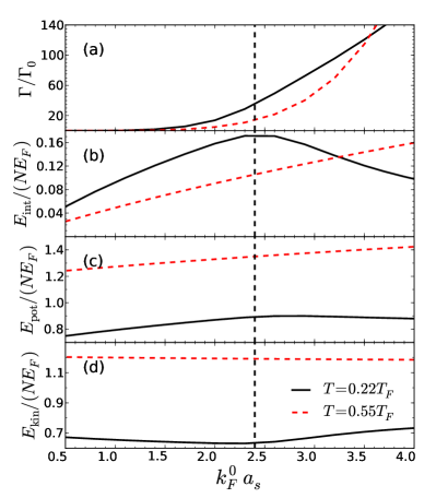
Figure 4: (Color online) Atom loss rate (a), interaction energy (b), potential energy (c), and kinetic energy (d) at different temperatures $T=0.22T_{F}$ (solid lines) and $T=0.55T_{F}$ (dashed line), with a total number of atoms $N=10^{4}$ and an imbalance ratio $p=0.10$.

There are very clear quantitative differences in the interaction energy, potential energy and kinetic energy in the ferromagnetic phase predicted by the two methods (see Figs. (3b), (3c), and (3d)). These differences are largely significant once the ferromagnetic domains are formed, and presumably are due to errors in the LDA treatment of the domain boundaries. Qualitatively, all the results from the two methods indicate a ferromagnetic phase transition at about $k_{F}^{0}a_{s}\approx 2.0$. The interaction energy and potential energy show a maximum at the transition, while the kinetic energy exhibits a minimum. Quantitatively, our mean-field prediction of the critical interaction strength is $(k_{F}^{0}a_{s})_{c}=1.93$. This is in good agreement with the MIT experimental finding of $(k_{F}^{0}a_{s})_{c}\simeq 2.2$ at the same temperature $T=0.12T_{F}$.

However, this agreement may simply be a coincidence. Monte-Carlo methods that take fluctuations into account predict a lower critical strength. Mean-field theory is not quantitatively reliable at these large interaction strengths with $k_{F}^{0}a_{s}\geq 1$. A possible explanation for the apparent coincidence is that the experimentally determined critical strength may not accurately correspond to the true, equilibrium critical strength. The recent measurements were carried out dynamically. In this type of non-equilibrium state, critical slowing-down and hysteresis-like effects will prevent ferromagnetic domains from immediately forming, and may push the effective critical interaction strength to a higher value.

The critical interaction strength also depends crucially on temperature. In Fig. (4), we graph the temperature dependence of the atom loss rate and energies. At higher temperatures, $T=0.22T_{F}$, the mean-field critical interaction strength increases to $(k_{F}^{0}a_{s})\simeq 2.4$,. This is much smaller than the experimental result of $(k_{F}^{0}a_{s})_{c}\simeq 4.2$, at the same temperature. For an even higher temperature, $T\simeq 0.55T_{F}$, there is no non-monotonic behavior in our mean-field results of the atomic loss and energies and, therefore no indication for the phase transition anymore. This is in agreement with experimental observation.

We finally consider the chemical potentials as shown in Figs. (3e) and (3f). The chemical potential increases with interaction strength and nearly saturates in the ferromagnetic phase. The same saturation was qualitatively observed in the MIT experiment ketterle2009Science .

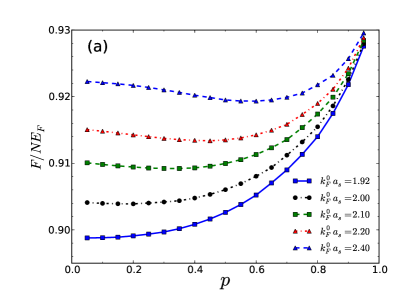
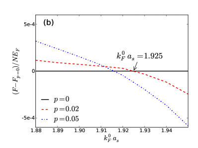
Figure 5: (Color online) (a) Free energy as a function of spin polarization $p$ for different interaction strengths: $k_{F}^{0}a_{s}=1.94,$ $2.00$, $2.10$, $2.20$, $2.40$ and $3.0$. (b) Free energy vs interaction strength $k_{F}^{0}a_{s}$ for different spin imbalances: $p=0.05$, $0.10$ and $0.20$. Here, $N=10^{4}$ and $T=0.12T_{F}$.

III.4 Critical interaction strength from the shape of free energy curve

At a finite temperature, we can accurately determine the critical interaction strength from the free energy, which should exhibit a minimum at non-zero magnetization. We present in Fig. (5a) the free energy as a function of spin polarization at different interaction strengths. For a weak interaction strength, for example $k_{F}^{0}a=1.92$, the free energy increases monotonically with spin polarization. Since the free energy should be symmetric (same) for $\pm p$, we simply refer this monotonic dispersion to as “U” shape. When the interaction is large enough, the state with a nonzero spin polarization becomes energetically favored (see, e.g., $k_{F}^{0}a_{s}=2.4$). Thus, the dispersion is changed to a “W” shape. As shown in Fig. (a5a), the position of the minimum shifts to large spin polarization with increasing interaction strength.

To determine the interaction strength accurately for this shape change, we calculate the free energy $F_{p}$ at three small spin polarizations: $p=0$, $0.02$ and $0.05$ near $k_{F}^{0}a_{s}=2.0$. In Fig. (5b), and show the free energy with respect to the non-polarization value $F_{p=0}$. We identify a crossover point at $k_{F}^{0}a_{s}=1.93$, above (below) which the state with spin polarization is lower (higher) in free energy. This is the critical interaction strength. For these atom numbers, our mean-field critical strength is the same as the LDA prediction for a trapped repulsive Fermi gas at the same temperature.

IV Conclusions

In conclusion, we have performed a self-consistent Hartree-Fock mean-field study of itinerant ferromagnetism for a harmonically trapped Fermi gas with strongly repulsive interactions. Our results for the density profiles, equations of state, and atom loss rate have been used to examine the validity of the widely used local density approximation. We have found that the local density approximation works fairly well below the ferromagnetic phase transition, and gives the same prediction for the critical coupling strength. However, in the ferromagnetic or spatially inhomogeneous phase, it gives quantitatively different predictions for both the equations of state and the atom loss rate, even for numbers of atoms as large as $N=10^{5}$. This discrepancy between the local density approximation and the more precise Hartree-Fock mean-field predictions is apparently due to the breakdown of the local density approximation at both the phase-separation boundary and at the edge of the trap.

This failure of the local density approximation is likely to remain an important issue even if we apply the local density approximation to the more accurate quantum Monte Carlo data obtained from a homogeneous ferromagnetic Fermi system. For this reason, it would be very useful to perform an inhomogeneous quantum simulation in the presence of a harmonic trap, in order to extend the present work beyond the mean-field approximation.

Our study may be useful for calculating the stiffness in the magnetization gradient term, which is also beyond the LDA. The stiffness has been computed phenomenologically in ref. LeBlancPRA09 using a Landau-Ginzburg expansion for the excess energy. For the normal-superfluid interface of a population imbalanced Fermi gas in the unitarity limit, it was shown that this expansion of gradient terms leads to about a factor-of-two error at zero temperature, compared with the full mean-field Bogoliubov-de Gennes calculation Baur2009PRA . We thus anticipate that our Hartree-Fock mean-field calculation will determine a similar stiffness as derived in LeBlancPRA09 , with a similar order of magnitude. However, a complete determination of the stiffness term is numerically challenging Baur2009PRA , especially at finite temperatures.

- (1) E. C. Stoner, Proc. R. Soc. London. Ser. A 165, 372 (1938).
- (2) L. Salasnich, B. Pozzi, A. Parola, and L. Reatto, J. Phys. B: At. Mol. Opt. Phys. 33, 3943 (2000).
- (3) T. Sogo and H. Yabu, Phys. Rev A 66, 043611 (2002).
- (4) R. A. Duine and A. H. MacDonald, Phys. Rev. Lett. 95, 230403 (2005).
- (5) S. Zhang, H.-H. Hung, and C. Wu, arXiv: 0805.3031 (2008).
- (6) J. L. LeBlanc, J. H. Thywissen, A. A. Burkov, and A. Paramekanti, Phys. Rev. A 80, 013607 (2009).
- (7) G. B. Jo , Y. R. Lee, J. H. Choi, C. A. Christensen, T. H. Kim, J. H. Thywissen, D. E. Pritchard, and W. Ketterle, Science 325, 1521 (2009).
- (8) T. Bourdel, J. Cubizolles, L. Khaykovich, K. M. F. Magalha, S. J. J. M. F. Kokkelmans, G. V. Shlyapnikov and C. Salomon, Phys. Rev. Lett. 91, 020402 (2003).
- (9) G. J. Conduit and B. D. Simons, Phys. Rev. Lett. 103, 200403 (2009).
- (10) H. Zhai, Phys. Rev. A 80, 051605(R) (2009).
- (11) G. J. Conduit, A. G. Green, and B. D. Simons, Phys. Rev. Lett. 103, 207201 (2009).
- (12) B. M. Fregoso and E. Fradkin, Phys. Rev. Lett. 103, 205301 (2009).
- (13) X. Cui and H. Zhai, Phys. Rev. A 81, 041602(R) (2010).
- (14) S. Pilati, G. Bertaina, S. Giorgini, and M. Troyer, arXiv: 1004.1169 (2010).
- (15) S.-Y. Chang, M. Randeria, and N. Trivedi, arXiv: 1004.2680 (2010).
- (16) T. N. De Silva and E. J. Mueller, Phys. Rev. Lett. 97, 070402 (2006).
- (17) A. Imambekov, C. J. Bolech, M. Lukin, and E. Demler, Phys. Rev. A 74, 053626 (2006).
- (18) X.-J. Liu, H. Hu, and P. D. Drummond, Phys. Rev. A 76, 043605(2007);
- (19) J. Reidl, A. Csordás, R. Graham, and P. Szépfalusy, Phys. Rev. A 59, 3816(1999).
- (20) D. S. Petrov, Phys. Rev. A 67, 010703(R) (2003).
- (21) S. K. Baur, S. Basu, T. N. De Silva, and E. J. Mueller, Phys. Rev. A 79, 063628 (2009).