Enhancement of nonclassical properties of two qubits via deformed operators

Abstract

We explore the dynamics of two atoms interacting with a cavity field via deformed operators. Properties of the asymptotic regularization of entanglement measures proving, for example, purity cost, regularized fidelity and accuracy of information transfer are analyzed. We show that the robustness of a bipartite system having a finite number of quantum states vanishes at finite photon numbers, for arbitrary interactions between its constituents and with cavity field. Finally it is shown that the stability of the purity and the fidelity is improved in the absence of the deformation parameters.

I Introduction

In the recent past, there has been a great deal of interest in the study of information transfer in connection between several physical fields nie00 . Using classical communication between two spatially separated parties, Pramanik et al pra10 have introduced a new scheme which is implemented by a sequence of unitary operations along with suitable spin-measurements. This protocol demonstrated the possibility of using intra-particle entanglement as a physical resource for performing information theoretic tasks. Di Franco and others fra10 have proposed a strategy for perfect state transfer in spin chains based on the use of an un-modulated coupling Hamiltonian whose coefficients are explicitly time dependent. They have shown that, if specific and non-demanding conditions are satisfied by the temporal behavior of the coupling strengths, their model allows perfect state transfer.

In a one-dimensional coupled resonator waveguide, an efficient scheme for the implementation of quantum information transfer has been given li09 . It has shown that quantum information could be transferred directly between the opposite ends of the coupled waveguide without involving the intermediate nodes via either Raman transitions or the stimulated Raman adiabatic passages. Further, quantum information transfer from spin to orbital angular momentum of photons has been also discussed by Nagali et al nag09 . On the other hand, many physical applications have been investigated on the basis of the $q$-deformation of the Heisenberg algebra (lav08 -fin96 ). In Ref. lav06 , a $q$-deformed Poisson bracket, invariant under the action of the $q$-symplectic group, has been derived and a classical $q$-deformed thermostatistics has been proposed in Ref. lav07 . In this sense one can say that, quantum entanglement is fundamental in quantum physics both for its essential role in understanding the non locality of quantum mechanics ein35 ; bel64 as well as for its practical application in quantum information processing nie00 ; ben00 . It is a kind of counter intuitive non local correlation.

The main purpose of this paper is to examine the effect of the $q$-deformation on transferring the information between two parties. This may be achieved if we considered one of the most generalized Hamiltonian which describes the interaction between pair of qubits and an electromagnetic field. In this case it is essential to include the effect of the $q$-deformation in the structure of the Hamiltonian through the dynamical operators. In the meantime, one of our target is to see the effect of the multiphoton process on the system. This means that, the model we plane to introduce should contains the effect of multiphoton in addition to the $q$-deformation. For this reason we devote the next section to introduce our model and to give the solution for the time-dependent wave function. In section III we consider the purity from which we discuss the degree of mixture for the system. We devote section IV to examine the accuracy of the information transfer against the scaled time. This is followed by our consideration of the population in section V. Finally we give our conclusion in section VI.

II The model

We consider the interaction between two qubits and a multiphoton cavity field. This Hamiltonian can be written in the following form

$$\frac{\mathrm{\hat{H}}}{\hslash}=\omega\hat{A}^{\dagger}\hat{A}+\sum_{i=1}^{2}\left(\frac{\Omega_{i}}{2}\hat{S}_{z}^{(i)}+\lambda\left(\hat{S}_{+}^{(i)}\hat{A}^{m}+\hat{S}^{(j)}\hat{A}^{\dagger m}\right)\right),$$ (1)

where $\omega$ is the frequency of the field. $\hat{A}$ and $\hat{A}^{\dagger}$ are the deformed annihilation and creation operators defined by

$$\hat{A}=\hat{a}f(\hat{n}),\quad\ \hat{A}^{\dagger}=f(\hat{n})\hat{a}^{\dagger},$$ (2)

where $f(\hat{n})$ is a function of the number operator $\hat{n}=\hat{a}^{\dagger}\hat{a}.$ The operators $\hat{a}$ and $\hat{a}^{\dagger}$ are the usual bosonic annihilation and creation operators with the property $\left[\hat{a},\hat{a}^{\dagger}\right]\ =1$ In the meantime the deformed operators $\hat{A}$ and $\hat{A}^{\dagger}$ satisfy the commutation relation

$$\left[\hat{A},\hat{A}^{\dagger}\right] = \left(\hat{n}+1\right)f^{2}\left(\hat{n}+1\right)-\hat{n}f^{2}\left(\hat{n}\right)\text{,}$$

$$\left[\hat{A},\hat{n}\right] = \hat{A},\qquad\left[\hat{A}^{\dagger},\hat{n}\right]=-\hat{A}^{\dagger}.$$ (3)

The operators $\hat{S}_{\pm}^{(i)}$ and $\hat{S}_{z}^{(i)},i=1,2$ are the usual raising (lowering) and inversion operators for the two-level atomic system, satisfying the relations

$$\left[\hat{S}_{z}^{(i)},\hat{S}_{\pm}^{(j)}\right]=\pm 2\hat{S}_{\pm}^{(i)}\delta_{ij}\qquad\text{and\qquad}\left[\hat{S}_{+}^{(i)},\hat{S}_{-}^{(j)}\right]=\hat{S}_{z}^{(i)}\delta_{ij},$$ (4)

where $\delta_{ij}$ is the Kronecker delta so that $\delta_{ij}=1$ if $i=j$ and $zero$ otherwise. To reach our goal we have to find the explicit expression of the wave function in the Schrödinger picture. For this reason we employ the Heisenberg equations of motion together with the Hamiltonian (1) that to derive some constants of motion from which we are able to achieve our task. In this case we have

$$\frac{d{\hat{S}_{z}^{(i)}}}{dt} = 2i\lambda(\hat{S}_{-}^{(i)}\hat{A}^{\dagger m}-\hat{S}_{+}^{(i)}\hat{A}^{m}),\qquad\frac{d\hat{A}}{dt}=-i\omega\hat{A}-i\lambda m\hat{A}^{\dagger(m-1)}\sum_{i=1}^{2}S_{-}^{(i)},$$

$$\frac{d\hat{A}^{\dagger}}{dt} = i\omega\hat{A}^{\dagger}+i\lambda m\hat{A}^{(m-1)}\sum_{i=1}^{2}S_{-}^{(i)}.$$ (5)

From the above equations we can deduce that

$$\hat{M}=\hat{N}+\frac{m}{2}\sum_{i=1}^{2}{\hat{S}_{z}^{(i)},\qquad}\hat{N}=\hat{A}^{\dagger}\hat{A},$$ (6)

where $\hat{M}$ is a constant of motion and $\hat{N}$ is the number of photon of the deformed operator $\hat{A}$. Using Eq.(6), the deformed Hamiltonian $\mathrm{\hat{H}}$ becomes,

$$\frac{\mathrm{\hat{H}}}{\hslash}=\hat{M}+\sum_{j=1}^{2}\hat{C}_{j},\quad\text{where\qquad}\hat{C}_{j}=\frac{\Delta_{j}}{2}\hat{S}_{z}^{(i)}+\lambda\left(\hat{S}_{+}^{(i)}\hat{A}^{m}+\hat{S}^{(j)}\hat{A}^{\dagger m}\right),$$ (7)

where $\Delta=\Omega_{j}-m\omega$ is the detuning parameter. Since the Hamiltonian given by equation (1) is a constant of motion, therefore the operator $\hat{C}_{j}$ is also constant of motion and consequently $\hat{M}$ and $\hat{C}_{j}$ are commute. To find the state vector $|\Psi(t)\rangle$ we assume that the initial atomic state takes the form

$$|\Psi(0)\rangle_{1,2}=a_{1}|e,e\rangle+a_{2}|e,g\rangle+a_{3}|g,e\rangle+a_{4}|g,g\rangle,$$ (8)

where the suffix $1$ and $2$ refers to the first and the second qubit, while $|e\rangle$ and $|g\rangle$ are the excited and ground states, respectively. It should be noted that $a_{i},i=1,2,3,4$ are arbitrary complex quantities that satisfy the condition$\sum_{i=1}^{4}|a_{i}|^{2}=1.$ Now suppose we consider the field is prepared in the coherent state

$$|\alpha\rangle=\sum_{n=0}^{\infty}Q_{n}|n\rangle\qquad\text{and\qquad}Q_{n}=\frac{\alpha^{n}}{\sqrt{n!}}\exp\left(-\frac{1}{2}|\alpha|^{2}\right).$$ (9)

Therefore, the initial state of the qubits and the field takes the form

$$|\Psi(0)\rangle_{s}=\sum_{n=0}^{\infty}Q_{n}\left(|\Psi(0)\rangle_{1,2}\right)\otimes|n\rangle.$$ (10)

In this case if we use the Schrödinger equation $i\hslash\partial|\Psi\rangle/\partial t=\mathrm{\hat{H}}|\Psi\rangle$ and the Hamiltonian (7) together with the above equation, then after some calculations the state vector of the system at $t>0$ can be written thus

$$|\Psi(t)\rangle_{s}=\sum_{n=0}^{\infty}A_{n}(t)|e,e,n\rangle+B_{n}(t)\left(|e,g,n+2\rangle+C_{n}(t)|g,e,n+2\rangle\right)+D_{n}(t)|g,g,n+4\rangle,$$ (11)

where $A_{n}(t),B_{n}(t),C_{n}(t)$ and $D_{n}(t)$ are complex time-dependent functions have the expressions

$$A_{n}(t) = a_{1}Q_{n}-\nu_{1}\left(a_{1}\nu_{1}Q_{n}+a_{4}\nu_{2}Q_{n+2}\right)\frac{\sin^{2}\mu_{n}t}{\mu_{n}^{2}}-i\nu_{1}(a_{2}+a_{3})Q_{n+1}\frac{\sin 2\mu_{n}t}{2\mu_{n}t},$$

$$B_{n}(t) = Q_{n+1}\left(a_{2}\cos^{2}\mu_{n}t-a_{3}\sin^{2}\mu_{n}t\right)-i\left(a_{1}\nu_{1}Q_{n}+a_{4}\nu_{2}Q_{n+2}\right)\frac{\sin\mu_{n}t}{2\mu_{n}t},$$

$$C_{n}(t) = Q_{n+1}\left(a_{3}\cos^{2}\mu_{n}t-a_{2}\sin^{2}\mu_{n}t\right)-i\left(a_{1}\nu_{1}Q_{n}+a_{4}\nu_{2}Q_{n+2}\right)\frac{\sin\mu_{n}t}{2\mu_{n}t},$$

$$D_{n}(t) = a_{4}Q_{n+2}-\nu_{1}\left(a_{1}\nu_{2}Q_{n}+a_{4}\nu_{2}Q_{n+2}\right)\frac{\sin^{2}\mu(n)t}{\mu_{n}^{2}}-i\nu_{2}(a_{2}+a_{3})Q_{n+1}\frac{\sin 2\mu_{n}t}{2\mu_{n}t}.$$

In the above equation we have used the abbreviations

$$\nu_{1}(n) = \lambda\sqrt{\frac{\left(n+m\right)!}{n!}G\left(n+m\right)},\quad\nu_{2}(n)=\lambda\sqrt{\frac{\left(n+m\right)!}{n!}G\left(n+2m\right)},$$

$$\mu(n) = \frac{1}{\sqrt{2}}\sqrt{\nu_{1}^{2}(n)+\nu_{2}^{2}(n)},\quad G\left(n+m\right)=f(n)f(n+1)f(n+2).......f(n+m).$$

It should be noted that in the previous calculations we have restricted ourself with the resonance case such that $\Delta=0.$ This is due to the fact that the solution in presence of the detuning parameter ($\Delta\neq 0$ ) is too cumbersome to be handled. Having obtained the state vector of the system, we are therefore in a position to find the density matrix $\hat{\rho}=|\Psi\rangle\langle\Psi|.$ On the other hand, there are several types of the function $f(n)$ would causes a deformation, one of them is called $q$-deformation. In this context we restrict ourselves with a case in which the function$\ f(n)$ is defined by

$$f(n)=\sqrt{\frac{1-q^{n}}{n(1-q)}}.$$ (14)

This in fact would help us to examine the effect of the $q$-parameter on the present system during our discussion for some statistical aspects.

III Degree of mixture

It is well known that, if the degree of mixture increases, then the quantum states tend to have a small amount of the entanglement. In the meantime for the case of pair of qubits, the states with a large enough degree of mixture are always separable kar ; Mun ; bat . There are several methods to measure the degree of mixture, among these methods we mention here, the von Neumann entropy of the state which is given by $\mathcal{S}=\hat{\rho}\ln\hat{\rho}$, this in addition to the linear entropy Bose besides the purity $\mathcal{P}$. Since the tasks of quantum information and computations require transferee information between two different locations as in quantum teleportation Ben ; bosc ; Lee or between two nodes as in quantum computations kay , therefore we have to investigate the behavior of the purity of the carrier of the information $\mathcal{P}$. This means that, the later method can be adopted to discuss the degree of mixture for the present system, where $\mathcal{P}=Tr\{\hat{\rho}^{2}\}$ and $\hat{\rho}$ is the density operator. In this case if one uses equation (11) the degree of purity for the qubits takes the form

$$\mathcal{P}(t) = |A_{n}(t)|^{2}+|B_{n}(t)|^{2}\left(1+|A_{n+2}(t)|^{2}+2|C_{n}(t)|^{2}\right)$$ (15)

$$+|C_{n}|^{2}\left(1+|A_{n+2}(t)|^{2}\right)+|D_{n}(t)|^{2}\left(1+2|A_{n+4}(t)|^{2}+2|B_{n+2}(t)|^{2}\right).$$

In what follows we investigate the effect of the deformed operators on the degree of the purity $\mathcal{P}$ provided that, the system is initially prepared in one of the Bell’s states. This type of states is defined as a maximally entangled quantum state of two qubits nie00 . In this context, we compare the effect of the deformed operator on $\hat{\rho}_{\psi}=|\psi\rangle\langle\psi|$ and $\hat{\rho}_{\phi}=$ $|\phi\rangle\langle\phi|$, where

$$|\psi\rangle=\frac{1}{\sqrt{2}}\left(|e,g\rangle+|g,e\rangle\right)\qquad\text{and}\qquad|\phi\rangle=\frac{1}{\sqrt{2}}\left(|e,e\rangle+|g,g\rangle\right).$$ (16)

As one can see it is quite difficult to analyze equation (15), this is due to the complication in the expression of the functions $A_{n}(t),B_{n}(t),C_{n}(t)$ and $D_{n}(t).$ For this reason we plot some figures to display the behavior of the purity related to the state $|\psi\rangle$. For example in figures (1) we have plotted the purity $\mathcal{P}(t)$ against the scaled time $\lambda t$ for different values of the involved parameters. In the absence of the effect of the $q$-deformation, namely $f(\hat{n})=1$ and for a fixed value of the mean photon number $|\alpha|^{2}=10,$ we have considered the cases in which the number of photons $m=1,2.$ In this case the purity starts with its maximum ( $\mathcal{P}(t)=1$ ) and as the time increases as its value decreases. Moreover, we observe irregular rapid fluctuations, this is depicted in Fig.(1a). Increasing the value of the number of photon $m=2,$ the function shows also rapid fluctuations, however, with interference between the pattern. In fact these fluctuations occur between the maximum value of the purity and its minimum around the value $0.45,$ see Fig.(1b). On the other hand, the behavior of the function is different when the $q$-deformation takes place, this is seen in Figs.(1c,d). In this case we have considered different values for the $q$ parameter, $q=0.1,0.5$ and $0.9.$ As we can see the general behavior of the purity is the same for all the cases, where the function decreases its value as the time increases, see Fig.(1c).

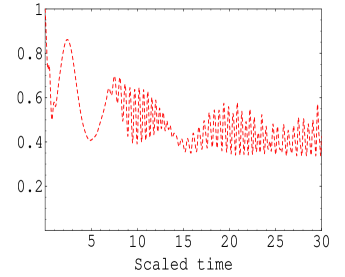
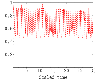
Figure 1: The purity $\mathcal{P}$ for the state $|\psi\rangle$ where $\bar{n}=10$. (a) $m=1$ (b)$m=2$ (c)$m=1$, the dash-dot, solid and the dot curves for $q=0.1,0.5,0.9$ respectively(d) the same as (c) but $m=2$.

In the meantime, we observe different behaviour for each case individually. For small values of the deformity parameter $q$, the amplitudes of the oscillations are small while the maximum values of the purity are too large. As one increases the deformity parameter, the purity function fluctuates rapidly and the amplitude of the fluctuations are large. This behavior causes a decrease of the minimum value of the purity as shown in Fig.(1c). More preciously when we consider $q=0.1$ (dash-dot curve), the purity displays regular fluctuations with an decrease in its value up to a certain limit. Then the function rebounds to increase its value without reaching its maximum. Similar behaviour is reported for the case in which $q=0.5$ (solid curve ), however, the increment in its value is less than that the previous case. More increases in the value of the $q$-deformation parameter leads to more decrease in the value of the purity. This is observed for the case in which $q=0.9$ (dot curve), where we can also see irregular fluctuations around $0.4$ after considerable reduction in its value. For $m=2,$ the purity reduces its value after a short period of the time when we consider $q=0.1$ and $q=0.5$, however, after onset of the interaction for $q=0.9$. As previously mentioned the function shows irregular fluctuations with an decrease in its value as the time increases. For the cases in which $q=0.1$ and $q=0.5$ the function turns to increase its value after a period of the time shorter than that the case in which $m=1$. Also we observe that, for small values of $q$ the purity oscillates faster but with small amplitudes. This behavior improves the purity, where its minimum value is always greater than that the free deformations. Here we can report that for $q=0.9$ there are more rapid fluctuations compared with the case in which $m=1.$ The same behaviour can also reported for the other two values for the $q$-deformation when $m=2$. In the meantime, the minimum values of these fluctuations are nearly bounded as can be seen in Fig.(1d). Now we turn our attention to display the dynamics of the purity for the second type of Bell state vector $|\phi\rangle$. In this case and for $m=1$ we observe that, there is a reduction in the value of the purity for all values of the deformed parameter $q$, however, with a different ratio. For example the function decreases its value after onset of the interaction for the case in which $q=0.9,$ while for the other two cases $q=0.1$ and $q=0.5,$ the reduction occurs after a short period of the time. Moreover, the reduction for the case in which $q=0.9$ is too large compared with the other two cases. In the meantime the rapid fluctations occurs in this case too, see Fig.(2a). When we examine the case in which $m=2$ the purity shows more decreases in its value with rapid fluctuations for all the values of the $q$ parameter. However, it is noted that for the case in which $q=0.1$ there is a sudden change in the function behaviour after considerable value of the time. In this case the function decreases its value without fluctuations after nearly half period of the considered time, see Fig.(2b).

From figures (1) and (2), we can conclude that, the decreasing of the purity of the maximum entangled states $|\psi\rangle$ and $|\phi\rangle$ is due to their interaction with the cavity mode. Although an increase in the number of photons within cavity leads to decrease the stability of the purity, however, it also improves its maximum and minimum values. Therefore, the deformed operators would enhance the purity of the traveling entangled states . Also we can report that, when the number of photons increases then the deformity parameter plays the role of error corrections with high efficiency.

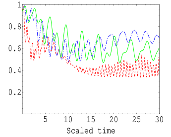
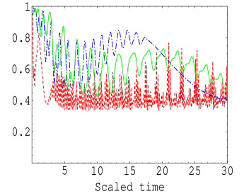
Figure 2: The same as Fig.(1c) and (1d) respectively but for the state vector $\bigl{|}\phi\bigr{\rangle}$

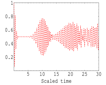
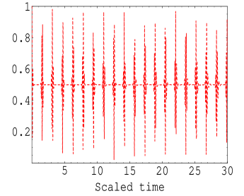
Figure 3: The fidelity of the travailing state $|\psi\rangle$ where $\bar{n}=10$ (a) For the free deformation with $m=1$(b) Free deformation and $m=2$ (c)Deformed case where the dash-dot, solid and dot curves for $q=0.1,0.5$ and $0.9$ respectively and $m=1$(d)The same as (c) but $m=2$

In the absence of $q$-deformation it is clear that the state $|\phi\rangle$ lose a large amount of purity compared with that for $|\psi\rangle$. This is seen in figures (1c) and (2a) where we also observe that, the purity for the state $|\psi\rangle$ is slow decaying compared with the second state $|\phi\rangle$ which shows fast decaying. In the presences of the deformation parameter in addition to the existence of more than one photon inside the cavity, the purity for both states is improved. Finally for the state $|\psi\rangle$ the minimum and maximum values are larger than those depicted for the state $|\phi\rangle$. This means that the state $|\psi\rangle$ is more robust than the state $|{\phi\rangle}$. Therefore, for the quantum information tasks it would be much better to find a suitable source to use it with Bell states of type $|\psi\rangle$ rather than the other Bell states.

IV Accuracy of information transfer

As well known quantum computing depends on transferring information from one nodes to another one subject to reach the final result. Therefore, it would be interesting to evaluate the fidelity of the transmitted information that is carried by the input state. The fidelity of the output information is given by

$$\mathcal{F}=tr\left(\hat{\rho}_{trans}\hat{\rho}_{out}\right),$$ (17)

where $\hat{\rho}_{trans}$ refers to the carrier of the transferred information and $\hat{\rho}_{out}$ is the carrier of the output information. In figures (3) we exhibit the dynamics of the fidelity of the transmit information which coded in the traveling state $|\psi\rangle$. For example, Fig.(3a) displays the behavior of $\mathcal{F}$ for non-deformed case in presence of a single photon within cavity, where $m=1$. In this case the fidelity shows behavior similar to that of the atomic inversion.

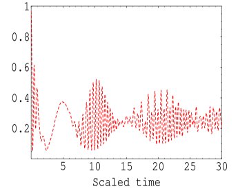
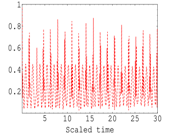
Figure 4: The same as Fig.(3) but for the travailing state $\bigl{|}\phi\bigr{\rangle}$.

This behavior usually appears as a result of the interaction between the field and the qubits within cavity. Increasing the number of the photons $m=2,$ regular fluctuations can be seen in the fidelity behavior with an increase in the function amplitude. This means that there is increasing in the periods of the collapses and revivals as depicted in Fig.(3b).

We now turn our attention to consider the case in which $m=1$ to see the effect of the deformation parameter $q$ on the fidelity $\mathcal{F}$ of the transfer information. As before, we have considered three different values of the $q$ parameter $q=0.1,0.5$ and $0.9.$ For the cases in which $q=0.1$ and $q=0.5,$ similar behavior can be reported, for example the function fluctuates and decreases its value as the time increases. However, for $q=0.1,$ the decreasing is faster than that the case in which $q=0.5$. Also we have realized that, the amplitude for the case $q=0.1$ is smaller than the case $q=0.5$. Moreover, the fluctuations in all the cases including $q=0.9$ occur around the value $0.5$. For the case in which $q=0.9$ different behavior can be seen. The function in this case decreases its value without fluctuations to reach its minimum below the value $0.4.$ However, after a considerable period of the time compared with the other two cases. Furthermore, as the time increases the function shows irregular fluctuations with an increase in its amplitude, see Fig.(3c).  When we increase the value of the photon number and consider $m=2$ we observe that, the function $\mathcal{F}$ decreases its value in addition to show rapid fluctuations after onset of the interaction for the case in which $q=0.9.$ This is followed with a period of revival and hence the function turns to display periods of rapid fluctuations with different amplitudes. In the meantime different observation can be reported for the other two cases $q=0.1$ and $q=0.5$. The function of the fidelity$\mathcal{F}$ in each case shows an decrease in its value with rapid fluctuations as the time increases. However, the amplitude of the fluctuations for $q=0.5$ is greater than that the case for which $q=0.1$, see Fig.(3d).

In Fig.(4), we investigate the dynamics of the fidelity for the state $|\phi\rangle$. In this case similar behavior can be seen as shown in Fig.(3). However, the function reduces its value and fluctuates just above the value $0.2$ not $0.5$ as in the previous case. Also there is a small period of oscillation occurs between two periods of the fluctuations which is not observed for the state $|\psi\rangle,$ see Fig.(4a). Increasing the photon number $m=2,$ more fluctuations can be reported besides the reduction in function value compared with the state $|\psi\rangle$ case, see Fig.(4b). Before we close this section we consider the effect of the $q$-deformation on the fidelity for the state $|\phi\rangle.$ This is depicted in figures (4c,d) where the function for the case in which $m=1$ and $q=0.1$ decreases its value faster than that the other two cases $q=0.5$ and $q=0.9$. Also in this case the function displays regular oscillations for $q=0.1$ and $q=0.5$, while it displays irregular fluctuations for the case in which $q=0.9$.  Furthermore, the function decreases its value as the time increases for $q=0.1$ and $q=0.5$, but it turns to increase its value slightly for the case in which $q=0.9$, see Fig.(4c). When we consider the case $m=2$, we observe for all values of the $q$-deformation parameter that, there are increasing in the fluctuations compared with the case in which $m=1$, see Fig.(4d).

In conclusion, the number of photons as well as the deformity play a role to enhance the fidelity of the transferee information. As it is shown, the fidelity of the traveling state in the presences of deformation is better than that the case of the free deformation. Increasing the number of photons inside the cavity, the fluctuations of the fidelity increase, however, with a small amplitude. Although the fidelity decreases as one increases the number of photons in the presences of the deformation parameter, however it does not tend to zero as we have shown.

Since the type of the traveling state plays an important role on the dynamics of the fidelity. Therefore, it is important to compare different types of input states which carry the required information. This means that we have to choose which one can resist during the traveling from one node to another, where the traveling environment is not perfect.

V Populations

Investigating the separability as well as the entanglement behavior of the traveling state is important for quantum information protocols. For this reason we have plotted figures (5) for different values of the involved parameters that to examine the probability distributions $P_{gg},P_{eg},P_{ge}$ and $P_{ee}$ for finding the traveling state $|\psi\rangle$ in the states $|g,g\rangle,|e,g\rangle,|g,e\rangle$ and $|e,e\rangle,$ respectively.  In Fig.(5a) we display the dynamics of the populations in absence of the deformation parameter and in the presence of a single photon within cavity. It is clear that the populations $P_{eg}$ and $P_{ge}$ (solid green curve) are coincide during the whole period of the interaction, while $P_{ee}$ (dash-dot blue curve) and $P_{gg}$ (dot red curve) have also the same behavior during the considered time. Here we emphasis on the fact that the main difference between $P_{eg}$ , $P_{ge}$ and $P_{ee},$ $P_{gg}$ is just phase during the oscillation periods. This means that the evolvement of the state $|\psi\rangle$ may takes for a small value of the scaled time the form

$$|\psi\rangle=\alpha\left(|e,g\rangle+|g,e\rangle\right)+\beta\left(|e,e\rangle+|g,g\rangle\right).$$ (18)

However, as time increases the behavior of the populations gets more stable and the travailed state would takes the form

$$|\psi\rangle=\alpha\left(|e,g\rangle+|g,e\rangle\right)+\beta_{1}|e,e\rangle+\beta_{2}|g,g\rangle.$$ (19)

It should be noted that, during the period of the interaction the travailed state would switch between the above two states (18) and (19). In Fig.(5b) we display the dynamics of populations for the case in which $m=2$ in the absence of the $q$-deformation parameter. In this case the usual phenomena of collapse and revival are pronounced where the state vector shown stability during the period of the revival. On the other hand during the period of the collapse different structure appears where the state $|\psi\rangle$ completely turns into the state $|\phi\rangle$.

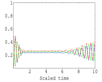
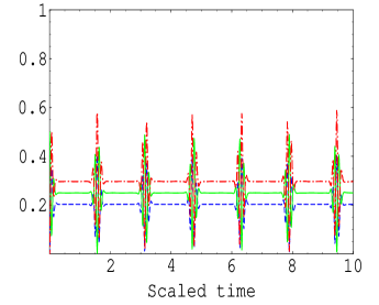
Figure 5: The population for the non-deformed case for the travailing state $|\psi\rangle$ where $\bar{n}=10$ and $m=1$ (a) The dash-dot, solid and the dot curves are for $P_{ee},(P_{eg}$ and $P_{ge})$ and $P_{gg},$ respectively (b) The same as (a) but for $m=2$.

To examine the effect of the $q$-deformation we have plotted figures (6) for different values of the $q$-deformation parameter as well as for the photon number $m$. For $m=1$ and $q=0.5$ the functions $P_{ee}$ and $P_{gg}$ are oscillating with different amplitude, however, both are in phase. While the functions $P_{eg}$ and $P_{ge}$ shown similar behavior but they exchange the oscillations with $P_{ee}$ and $P_{gg}$, see Fig.(6a). When we increase the value of the photon number, $m=2$ different behavior can be seen. In this case there are increasing in the number of the oscillations in all the population functions. However, there are also a clear difference between each population. For example the population $P_{ee}$ increases its amplitude corresponding to decrease in the amplitude of the population $P_{gg}.$ Furthermore, as the time increases as the amplitude of each function decreases. On the other hand we can observe the same behavior in the function $P_{eg}$, however, with different phase and amplitude, see Fig.(6b).

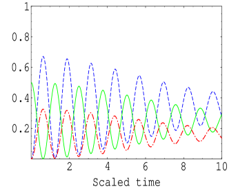
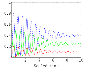
Figure 6: The same as Fig.(5), but for the deformed case (a) $m=1$ and $q=0.5$(b)$m=2$ and $q=0.5$(c) $m=1$ and $q=0.9$(d)$m=2$ and $q=0.9$

When we have examined the case in which $m=1$ and $q=0.9,$ similar behavior to the case in which $m=2$ and $q=0.5$ is observed. However, the amplitude for all the population functions are decreasing as the period of the time increases, see Fig.(6c). In crease the value of the $q$-deformation, $q=0.9$ leads to rapid fluctuations in all the population functions. This becomes more pronounced after certain period of the time, see Fig.(6d). Here we would like to emphasis on the fact that, as the amplitude of the populations decreases as the degree of entanglement increases.

Among the important forms which can be detected from figures (6) is the state

$$|\psi\rangle=\alpha_{3}\left(|e,g\rangle+|g,e\rangle+|e,e\rangle\right)+\beta_{3}|g,g\rangle,$$ (20)

which has a structure similar to that of equation (19) but with the supper position of the state $|e,e\rangle$ instead of the state $|g,g\rangle$

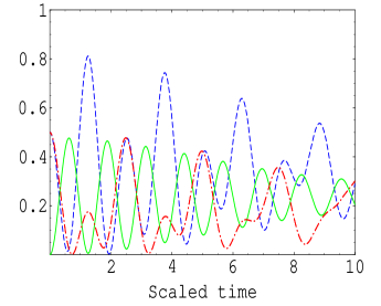
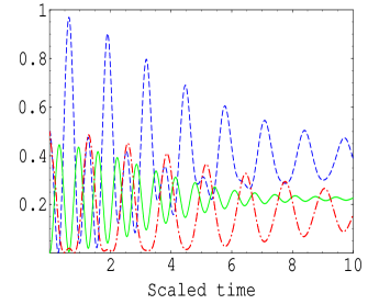
Figure 7: The same as Fig.(6a,b) but for the state vector $\bigl{|}\phi\bigr{\rangle}$

Finally we investigate the dynamics of the population for the state vector $|\phi\rangle$. To do se we have plotted figures (7) for fixed value of the $q$-deformation, $q=0.5$ and for $m=1,2$. In this case the populations $P_{ee}$ and $P_{gg}$ start with the value 0.5 after onset of the interaction where both functions show regular oscillations with a reduction in their values as the time increases. However, for the first period of the oscillations of the function $P_{gg}$ increases its value up to $0.8$. On the other hand the function $P_{eg}$ start with zero value and hence it starts to increase its value up to $\sim 0.5$ showing regular oscillations. Also we observe that, as the time increases as the function decreases its value and consequently the entanglement shows improvement for a large value of the time, see Fig.(7a). Increasing the value of the photon number, for example $m=2$ we observe an increase in the value of the amplitude, more precisely in the function $P_{ee}$ which approaches the maximum value of the population. In the meantime the function $P_{gg}$ shows regular fluctuations shrinking as the time increases. Similar behavior can also reported for the other two populations $P_{ee}$ and $P_{ge}.$ However, the oscillations in the function $P_{ge}$ are decaying faster than that the other two populations, see Fig.(7b).

VI Conclusion

In the present paper we have considered the problem of the interaction between two qubits and multi-photon cavity field. The creation and annihilation operators which describe the field are considered to be deformed. An exact analytical solution of the wave function is obtained and used to construct the density matrix operator. The effect of the number of photons in addition to $q$-deformation are examined where the investigation carried out on the purity, the fidelity of the travailing state and the population. We have shown that when the number of photons inside the cavity is increased the fluctuations as well as the amplitude of these functions are also increased. On the other hand the existence of the deformation leads to an enhancement of the fidelity and the purity for small values of the deformity parameter. However for large values of the $q$-deformation parameter, the minimum values are always bounded. As a result of the interaction between the qubits and the field, the structure of the travailing state would takes a different form. In addition, the nature of the structure can also causes a decrease in the purity and the fidelity. Therefore, the evolvement state loses some of its entanglement and turns into partially entangled state. This in fact encouraged us to examine the robustness of the travailing state and make a comparison between two different types of the maximum entangled Bell state. It has been shown that, the robust state is only pronounced in one of these states. This means that, coding the information in this robust state maybe more save during the evolvement to achieve quantum communication or computation tasks. Since it is possible to control the devices in the reality, therefore we belief that, the present results can give us an indication of how the carrier of information propagate from node to another node.

Acknowledgement:

One of us (M.S.A.) is grateful for the financial support from the project Math 2010/32 of the Research Centre, College of Science, King Saud University.

References

- (1) M. A. Nielsen and I. L. Chuang, Quantum Computation and Quantum Information (Cambridge University Press, Cambridge, England, 2000).
- (2) T. Pramanik, S. Adhikari, A.S. Majumdar, Dipankar Home, Alok Kumar, Physics Letters A 374, 1121 (2010)
- (3) C. Di Franco, M. Paternostro, M. S. Kim, Phys. Rev. A 81, 022319 (2010)
- (4) Peng-Bo Li, Ying Gu, Qi-Huang Gong, Guang-Can Guo, Phys. Rev. A 79, 042339 (2009)
- (5) Eleonora Nagali, Fabio Sciarrino, Francesco De Martini, Lorenzo Marrucci, Bruno Piccirillo, Ebrahim Karimi, Enrico Santamato, Phys. Rev. Lett. 103, 013601 (2009)
- (6) A. Lavagno, J. Phys. A: Math. Theor. 41, 244014 (2008).
- (7) J. Wess and B. Zumino, Nucl. Phys. B 18, 302 (1990)
- (8) E. Celeghini, et al. Ann. Phys. 241, 50 (1995)
- (9) B. L. Cerchiai, R. Hinterding, J. Madore and J. Wess, Eur. Phys. J. C 8, 547 (1999); Eur. Phys. J. C 8, 533 (1999).
- (10) V. Bardek and S. Meljanac, Eur. J. Phys. C 17, 539 (2000)
- (11) R. Finkelstein, J. Math. Phys. 37, 983 (1996); J. Math. Phys. 37, 2628 (1996).
- (12) A. Lavagno, A. M. Scarfone and N. P. Swamy, Eur. Phys. J. C 47, 253 (2006).
- (13) A. Lavagno, A. M. Scarfone and N. P. Swamy, J. Phys. A: Math. Theor. 40, 8635 (2007).
- (14) A. Einstein, B. Podolsky, and N. Rosen, Phys. Rev. 47, 777 (1935).
- (15) J. S. Bell, Physics 1, 195 (1964).
- (16) C. H. Bennett and D. P. Di Vincenzo, Nature 404, 247 (2000).
- (17) H. Bennett, G. Brassard, C. Crepeau, R. Jozsa, A. Pweres and W. K. Wootters, Phys. Rev. Lett. 70 1895 (1993)
- (18) D. Boschi, S. Branca, F.De Martini, L. Hardyband S. Popescu, Phys. Rev. Lett. 801121 (1998).
- (19) P. Shor, SIAM J. Comput 26 1484 (1997); L. Grover, Phys. Rev. Lett. 79 4709 (1997).
- (20) C. Bennett and S. Weisner, Phys. Rev. Lett. 69, 2881 (1992).
- (21) K. Mattle, H. Weinfurter, P. Kwiat, and A. Zeilinger, Phys. Rev. Lett. 76, 4656 (1996).
- (22) J.-W. Pan, D. Bouwmeester, H. Weinfurter, and A. Zeilinger, Phys.Rev. Lett. 80, 3891 (1998).
- (23) T. Jennewein, G. Weihs, J.-W. Pan, and A. Zeilinger, Phys. Rev. Lett. 88, 017903 (2002).
- (24) D. Bouwmeester, J. Pan, K. Mattle, M. Eibl, H. Weinfurter, and A. Zeilinger, Nature 390, 575 (1997).
- (25) K. Zyczkowski, P. Horodecki, A. Sanpera, and M. Lewenstein, Phys. Rev. A 58, 883 (1998); Karol Zyczkowski, Phys. Rev. A 60 3496 (1999).
- (26) W.J. Munro, D.F.V. James, A.G. White, and P.G. Kwiat, Phys. Rev. A 64, 030302 (2001).
- (27) J. Batlea, A. R. Plastinoa, M. Casas and A. Plastinob, Phys. Lett. A 298, 301 (2002).
- (28) S. Bose et al., Phys. Rev. A 61, 040101(R) (2000).
- (29) J. Lee and M. S. Kim, Phys. Rev. Lett. 84, 4236 (2000).
- (30) K. Phillip, Laflamme, Raymond; Mosca, Michele,” An introduction to quantum computing”, Oxford University Press, (2007).